FAST ALGORITHMS FOR BROWNIAN DYNAMICS WITH HYDRODYNAMIC INTERACTIONS
Wenhua Guan
A dissertation submitted to the faculty at the University of North Carolina at Chapel Hill in partial fulfillment of the requirements for the degree of Doctor of Philosophy in the Department of
Mathematics in the College of Arts and Sciences.
Chapel Hill 2016
c 2016 Wenhua Guan
ALL RIGHTS RESERVED
ABSTRACT
Wenhua Guan: Fast Algorithms for Brownian Dynamics with Hydrodynamic Interactions
(Under the direction of Jingfang Huang)
To my family!
ACKNOWLEDGEMENTS
Many thanks to the members of the Department of Mathematics of the University of North Carolina at Chapel Hill for their instruction, support, and encouragement.
I wish to single out my advisor, Dr. Jingfang Huang, for his exceptional patience, valuable guidance and generous support during my graduate study. Dr. Huang gave me a lot of freedom and allowed me to explore on my own, which greatly improved my ability to work independently and benefited me for my future career. His pursuit of optimal numerical results and dedication to research has a big influence on me and stimulated me. I am grateful to him for holding me to a high research standard which guaranteed the quality of work presented here.
I also wish to thank my committee, including Dr. Gary Huber, Dr. Laura Miller, Dr. Katie Newhall and Dr. Jan Prins. I am grateful to Dr. Jan Prins for providing me intelligent advice for this dissertation, for teaching me a lot of knowledge about parallel computing, and for giving me many suggestions about the job hunting. Discussion with him every time was full of pleasure and knowledge. His professionalism, dedication and kindness has greatly inspired me and encouraged me. I am thankful to my collaborator, Dr. Gary Huber for broadening my knowledge in biochemistry and biology, for reading and commenting on this dissertation. I also wish to thank Dr. Laura Miller for introducing me job opportunities, for writing references, and for helping me along the way. I thank Dr. Katie Newhall for her time and enthusiasm.
I thank Dr. Gregory Forest for supporting me in the final summer and taking every effort to help me finish my degree at UNC. I thank Dr. Xiaolin Chen for providing wonderful suggestions on my oral slides.
through the careful grammatical editing by Miss Strabue and Dr. Davidson. I would also thank the joyful moments from the lunch group(Dan, Feifei, Tim, Yan, Yuan, Wayne etc), as well as their consideration and support. Thank my office mates Yuan and Zeliha. Thank all the other friends who have helped me and encouraged me.
My sincere appreciation also goes to my master advisor, Dr. Bo Yu, for his constant support and encouragement all the time.
Most importantly, none of this would happen without the love and encouragement from the family. Thank my parents who raised me to value knowledge and supported me in all of my life endeavors. Their love and parenting helped me foster a solid work ethic and shaped the person I have become. I would like to thank my husband, Ming, who has made all the difference in my life, for believing me, loving me, encouraging me. His wisdom and knowledge enlightened me.
TABLE OF CONTENTS
LIST OF FIGURES . . . ix
LIST OF TABLES . . . x
CHAPTER 1: INTRODUCTION . . . 1
1.1 Background . . . 1
1.2 Ermak-McCammon Model for Spherical Particles . . . 3
1.3 Brownian Dynamics Model for Rigid Macromolecules of Arbitrary Shape . . . 7
1.4 Outline of the Dissertation . . . 10
CHAPTER 2: COMPUTATION OF ELECTRIC FIELD GRADIENTS BY FAST MULTIPOLE METHOD . . . 13
2.1 Adaptive Tree Structure for the Spatial Domain . . . 16
2.2 Approximation and Translation . . . 20
2.2.1 Mathematical Preliminaries . . . 20
2.2.2 Approximation Operators . . . 23
2.2.3 Translation Operators . . . 24
2.3 Local Expansions of the Fields and Electric Field Gradients . . . 29
2.3.1 Electrostatic Fields . . . 29
2.3.2 The far-field Electric Field Gradients . . . 32
2.4 Algorithm for Adaptive FMM . . . 37
2.5 Numerical Results . . . 41
2.5.1 Cube . . . 42
2.5.2 Surface of A Unit Sphere . . . 45
CHAPTER 3: ADAPTIVE ROTNE-PRAGER-YAMAKAWA SOLVER BY
MUL-TIPOLE METHODS . . . 49
3.1 Rotne-Prager-Yamakawa Tensor . . . 52
3.1.1 Far-field Rotne-Prager-Yamakawa Evaluation with Multipole Methods . . . . 53
3.1.2 Near-field Rotne-Prager-Yamakawa Potential Evaluation . . . 55
3.2 Adaptive Rotne-Prager-Yamakawa Algorithm with Multipole Methods . . . 56
3.3 Numerical Results . . . 57
3.3.1 Cylinder . . . 57
3.3.2 Eight Surface . . . 58
CHAPTER 4: HYDRODYNAMIC INTERACTIONS OF COMPLEX, RIGID, BI-OLOGICAL MACROMOLECULES IN SUSPENSION . . . 63
4.1 Hydrodynamic Interactions . . . 65
4.2 Bead-Shell Model . . . 65
4.3 Mathematical Formulation of the many-body System in Suspensions with Bead Model 66 4.4 Fast Algorithms for the many-body System . . . 70
4.4.1 Block Conjugate Gradient Method . . . 71
4.4.2 Numerical Results of the Block Conjugate Gradient Method . . . 71
4.4.3 Schur Complement Method . . . 73
4.4.4 Numerical Results of Schur Complement Method . . . 75
CHAPTER 5: CONCLUSION . . . 78
REFERENCES . . . 81
LIST OF FIGURES
2.1 Blue boxes are colleagues of box b and white boxes are the interaction list ofb. . . . 12
2.2 Box band its associated lists in two dimension . . . 13
2.3 The uplist of Box b [2] . . . 14
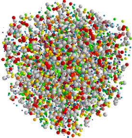
2.4 Charges randomly distributed in a cube . . . 33
2.5 Charges randomly distributed on the surface of the sphere . . . 36
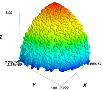
2.6 Charges randomly distributed on the surface of the first octant . . . 38
3.1 Particles randomly distributed on the surface of a cylinder . . . 46
3.3 Particles randomly distributed on an eight surface . . . 48
3.2 Speedup of particles randomly distributed on the surface of the cylinder . . . 49
3.4 Speedup of particles randomly distributed on the eight surface . . . 51
4.1 Complex biological macromolecule structures [4] . . . 53
4.2 (A) Atomistic DNA model (B) Bead Model with each DNA residue modeled with a single pseudoatom (C) Bead-shell model with surfaces covered with spherical elements(By Maciej Dlugosz [5]) . . . 54
4.3 Bead-shell model of the two body system . . . 59
4.4 Iteration number of the block conjugate gradient method for the hydrodynamics of the two-body system . . . 60
4.5 Bead-shell model of the two body system with different sizes . . . 62
4.6 Iteration number of Schur complement method for the hydrodynamics of the two-body system with different sizes . . . 62
4.7 Comparison of iteration number of Schur complement method with and without preconditioner for the hydrodynamics of the two-body system with different sizes . . 63
4.8 The bead-shell model of the many-body system with different sizes . . . 63
LIST OF TABLES
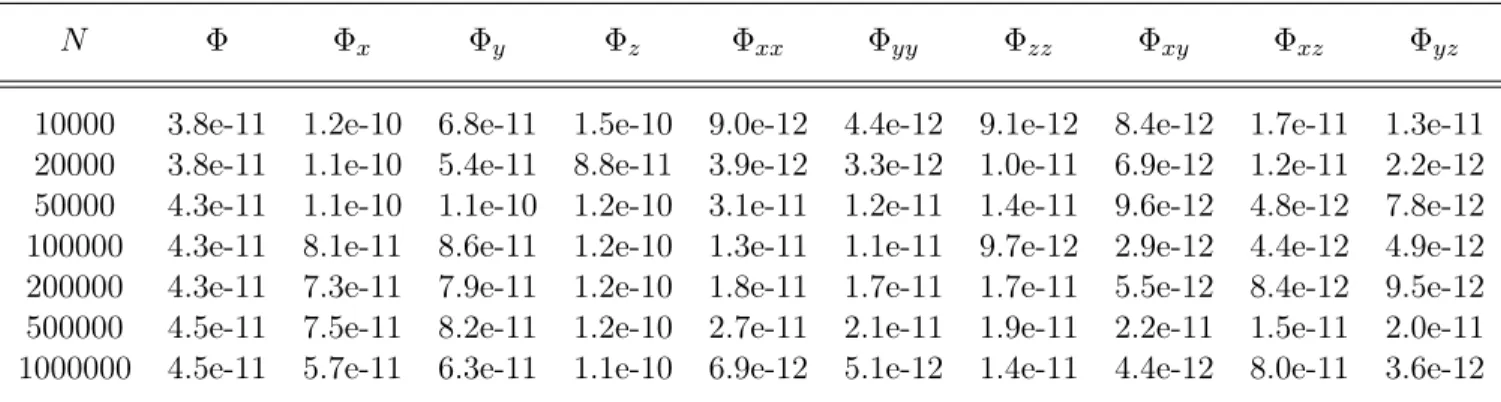
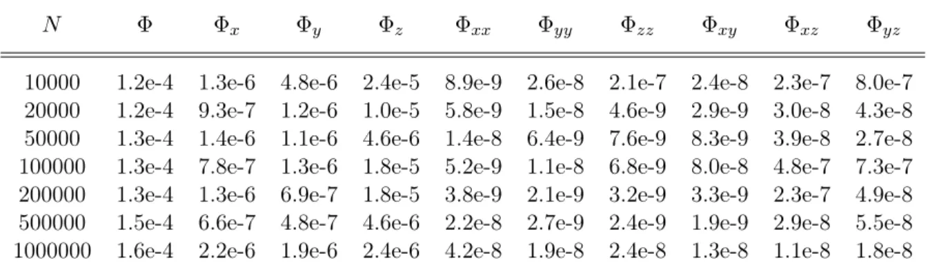
2.1 Error Results of the new version of FMM for 3-digit accuracy with charges randomly distributed in a cube . . . 33
2.2 Error results of the new version of FMM for 6-digit accuracy with charges randomly distributed in a cube . . . 34
2.3 Error results of the new version of FMM for 9-digit accuracy with charges randomly distributed in a cube . . . 34
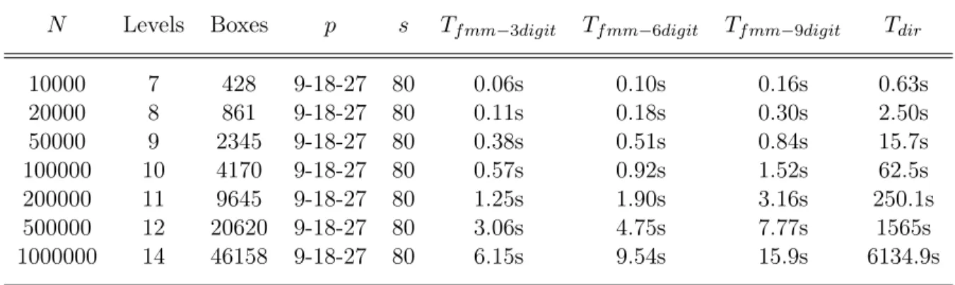
2.4 Timing results of the new version of FMM with charges randomly distributed in a cube 35
2.5 Error results of the new version of FMM for 3-digit accuracy with charges randomly distributed on the surface of a sphere . . . 36
2.6 Error results of the new version of FMM for 6-digit accuracy with charges randomly distributed on the surface of a sphere . . . 37
2.7 Error results of the new version of FMM for 9-digit accuracy with charges randomly distributed on the surface of a sphere . . . 37
2.8 Timing results of the new version of FMM with charges randomly distributed on the surface of a sphere . . . 37
2.9 Error results of the new version of FMM for 3-digit accuracy with charges randomly distributed on the surface of the first octant . . . 38
2.10 Error results of the new version of FMM for 6-digit accuracy with charges randomly distributed on the surface of the first octant . . . 38
2.11 Error results of the new version of FMM for 9-digit accuracy with charges randomly distributed on the surface of the first octant . . . 39
2.12 Timing results of the new version of FMM with charges randomly distributed on the surface of the first octant . . . 39
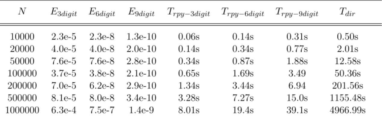
3.1 Numerical results of RPY solver for particles randomly distributed on the surface of the cylinder(12 threads) . . . 47
3.2 Running time of RPY solver of 6-digit accuracy for particles randomly distributed on the surface of the cylinder . . . 47
3.3 Speedup of RPY solver of 6-digit accuracy for particles randomly distributed on the surface of the cylinder . . . 48
3.4 Numerical Results of RPY solver for particles randomly distributed on the eight surface (12threads) . . . 49
3.5 Running time of RPY solver of 6-digit accuracy using different threads for particles randomly distributed on the eight surface . . . 50
CHAPTER 1 Introduction
1.1 Background
The interiors of all living cells are crowded with biological macromolecules, such as proteins, nuclear acids (RNA, DNA), carbohydrates, polymeric lipids and so on. Macromolecules are constantly moving around by diffusion in biological systems. Diffusion is basically the random motion of molecules which is driven by thermal energy. It is one of the fundamental questions that is being pursued by scientists in molecular biology, cellar biology and beyond. Molecules, macromolecules and nanoparticles, under diffusive transport in a fluid medium, is of interest in many biological applications, such as drug delivery and separation processes [6]. Moreover, a detailed study of the transport, regulation and dynamics of molecules inside cells can help us to understand how healthy cells change to disease states and provide important information to the developers of therapeutic drugs. Micro and nano drug delivery systems are developed to deliver the drug to the desired tissue in the human body so that it increases the efficiency and effectiveness of the treatment and minimizes the side effects associated with the drug [7]. Therefore, the understanding of these mechanisms will also help researchers to develop preemptive treatment, monitored by a wrist-worn device for detecting diseases. Recently, Google has been working on a nanoparticle pill that can identify cancers, heart attacks and other diseases before they become a problem.
individual molecules. Hence, the detailed information on the dynamic behaviors of both solute and solvent molecules are included in molecular dynamics at an atomic level of description. The molecular dynamics is more accurate compared with the other coarse-grained models. However, accounting for the effect of the solvent molecules on the solute will require a prohibitive computational cost for long-time simulations [9].
Brownian dynamics is a mesoscopic method for simulating the diffusive behavior of particles which undergoes Brownian motion in fluids. In Brownian dynamics, the solvent is treated as a continuum and the impact of the explicit solvent molecules to the solute molecules are replaced instead by an instantaneous friction force and a fluctuating force. The reason why the Brownian dynamics methods allow one to simulate much larger time scales than in molecular dynamics simulations is because Brownian dynamics techniques are able to coarse-grain out the fast modes of the solvent molecules [10]. The Brownian dynamics method takes the advantage of the large separation in time scales between the rapid motion of solvent molecules and the slow motion of the Brownian particles, the mass and size of which are larger than those of the host medium particles [11]. The core of the Brownian dynamics simulation is a first or second order stochastic differential equation in time for the position of the solute molecules which allows for studying the temporal evolution and dynamics of complex fluids. Brownian dynamics techniques have been widely used in biology, biochemistry, chemical engineering and materials sciences [12, 13]. It has many applications, such as protein folding [14, 15], DNA bending and supercoiling [16, 17, 18], steering in enzyme/substrate encounter [19, 20, 21, 22], and diffusion in crowded cells [23, 24].
the Brownian particles mediated by fast momentum transfer through the solvent since it will result in high computational cost. It may cause unphysical results as soon as the time scale exceeds a few collision times. Proper treatment of hydrodynamic interactions is essential in simulation studies of Brownian particles in the flow.
Given the ability of Brownian dynamics techniques in bridging different time and length scales, it becomes essential for developing fast algorithms in Brwonian dynamics simulations with hydrodynamic interactions to study the dynamics of macromolecules. Current algorithms for dynamical modeling fail to perform a simulation long enough to observe a large-scale conformational change. The massive number of parameters and iterations required to accurately model a reasonably-sized many-body system of macromolecules at proper resolution are beyond even the processing abilities of supercomputers. Understanding the interplay between different mechanisms at various scales presents formidable challenges to conventional mathematical modeling and solution techniques, and thus requires the development of accurate and robust multiscale models and efficient algorithms for simulations. Below, the Brownian dynamics model with hydrodynamic interactions will be presented for describing the motions of spherically symmetric particles and the associated computation challenges. The rotations of these particles can be neglected due to their symmetric geometry. Based on the model for spherical particles, the Brownian dynamics translational-rotational model for rigid macromolecules of arbitrary shape is described and the corresponding diffusion matrix has been calculated through the deformation of the macromolecules by bead-shell model.
The goal of this dissertation is to derive state-of-the-art fundamental algorithms to advance Brownian dynamics simulations with hydrodynamic interactions and implement the fast algorithms as solvers to accelerate the numerical simulations. These simulations will be suitable for a broad class of flows and physical scales and allowing for further simulating notable complex-structured macromolecules, as well as forcing terms.
1.2 Ermak-McCammon Model for Spherical Particles
Consider a suspension ofN identical spherical particles of radiusa, immersed in an incompressible
Newtonian fluid of viscosity ⌘ at low Reynold number. When the inertial relaxation times are short compared to the timescale of interest, it is often possible to ignore inertia in the governing equation.
A Langevin description of the N-particle system is presented below and a random force representing
the action of the thermal motion is added to Newton’s equation. Rotations of the particles will not be accounted for since they are spherically symmetric. For particle i, i= 1, . . . , N with translational
velocityVi, from Newton’s Second Law, there is
mi
dVi
dt =F
t
i =Fhi +FBi +Fnhi . (1.1)
Here, mi is the generalized mass of particlei. The total forceFti on particle iis composed of three
parts: the frictional force Fhi from the particle moving through the viscous solvent, a Brownian
force FBi due to the random successive collision of the solvent molecules with the Brownian particle,
and all deterministic non-hydrodynamic forceFnh
i for particlei. The non-hydrodynamic force is
also calledsystematic force which includes any external body force and force due to the interaction potential energy between Brownian particles, like the electrostatic interactions and Vander Waals interactions.
The hydrodynamic force Fhi acting on particle itends to decrease the energy and depends on
the appropriate components of the configuration-dependent tensor ⇣, which is called hydrodynamic friction tensor. Due to the linearity of the Stokes equations, the forces exerted by the fluid on the particles depend linearly on the translational velocities of the particles. This relation defines
Fhi =
N X
j=1
⇣ijdxj
dt . (1.2)
LetFh = [Fh1, . . . ,FhN]T,x= [x1, . . . ,xN]T be the hydrodyanmic forces and locations of all particles.
The above equation can be written as
Fh= ⇣dx
dt. (1.3)
According to the Stokes-Einstein relation, the N-particle diffusion tensorD and the friction tensor
⇣ has relation
D=kBT⇣ 1, (1.4)
wherekBis the Boltzman constant andT is the temperature. The diffusion tensor, a3N⇥3N dense
tensor or the Oseen tensor. The difference between these two tensors are elaborated in chapter 3. Notably, both the Roten-Prager-Yamakawa tensor and the Oseen tensor are divergence-free, which considerably simplifies the computation of Brownian dynamics models.
X
j
@Dij
@rj ⌘
0. (1.5)
The Brownian force FB
i (t) arising from the thermal fluctuations in the fluid and tending to
increase the energy of the particle is characterized by [26]
<FBi (t)>= 0
<FBi (t)FBj (s)>= 2kBT⇣ij (t s).
(1.6)
The angle brackets in Equation (1.6) denote an ensemble average. is the Dirac’s delta function. The amplitude of the correlation between the Brownian forces attandsresults from the
fluctuation-dissipation theorem for theN-body system. The time scale t researchers are interested in is longer
than⌧ =m/6⇡⌘a(momentum relax time of the particle after a Brownian impluse) but smaller than
the time the configuration changes. The fluctuating forces are considered instantaneous.
The evolution equation for the particles is described by following Ermak-McCammon model [11] by integrating Equation (1.1) over time step t. The displacement vector x for all small rigid
spherical particles during time step t due to the non-hydrodynamic force Fnh and the Brownian
forceFB is given by
x( t) = t
kBT
D·Fnh+R( t) +r·D t (1.7)
< R( t)>= 0, <R( t)R( t)>= 2D t. (1.8)
Equation (1.7) can also be obtained from Fokker-Planck or Smolochowski equation for the
N-particle probability distribution function. Equation (1.7) is the heart of the Brownian dynamic
simulations which describesN particles suspended in unbounded flow interacting through
hydro-dynamic, interparticle, external, and Brownian forces. It simply states that the displacement of a particle includes three parts. There is a deterministic contribution due to the non-hydrodynamic or systematic force, and two contributions from Brownian motion: a random displacement which
makes the fluctuation-dissipation theorem satisfied and a displacement due to the configuration-space divergence of theN-particle diffusivity r·D t. This term becomes zero when the diffusion matrix D is modeled by Oseen tensor and Roten-Prager-Yamakawa tensor because they are divergence-free.
For rigid, spherical particles without considering rotations, there are three computational chal-lenges for the Brownian dynamic simulations with hydrodynamic interactions :
1. The electrostatic field around the target molecule is only computed once at the initial step of the simulation due to prohibitive computational cost using existing methods. Such temporal approximation presents major limitations in accuracy of the simulations, especially in the situations when the ligand is not small in size, or the concentration of ions is high (as in real biological ranges), or when boundaries or interfaces are present. The Adaptive Fast Multipole Poisson-Boltzmann (AFMPB) solver [27] is an open-source software developed by Huang and the collaborators for solving the linearized Poisson-Boltzmann (LPB) equation which models the electrostatic interactions in biomolecular systems. AFMPB has significant improvements in computational efficiency and numerical stability over other existing LPB solvers.
2. The first term on the right side of Equation (1.7) is mainly a matrix-vector multiplication between the diffusion matrix and the non-hydrodynamic force. Direct evaluation of it will result inO(N2) complexity, whereN is the number of spherical particles. Additionally, since
the diffusion matrixD for spherical Brownian particles is configuration-dependent and dense,
explicit construction of it will result in high memory usage. For example, according to Liu and Chow [28], the memory storage for the diffusion matrixDof10Kparticles will be as huge as 32
GB, which is impracticable for large-scale and long-time simulation. To reduce the complexity for diffusion-force matrix-vector evaluation, various fast algorithms have been developed, for example, Ewald summation [29], Particle mesh techniques including the Particle Mesh Ewald (PME) method [30] and the Smooth Particle Mesh Ewald (SPME) method [31] with complexity
O(N logN). The other methods include Method of local corrections [32], multigrid methods [33], panel clustering method and precorrected-FFT [34], and fast multipole method [35].
factoriza-interactions for small scales. Matrix factorization techniquesD=B·BT and D=pD·pD
(Davis, 1987 [36]) require forming the diffusion matrixD explicitly and result in high memory
usage. Iterative methods based on Krylov subspace methods and Chebyshev approximations p
D·F ⇡ p(D)F are practical for large-scale time simulation if the fast evaluation of the
matrix-vector multiplication D·Fis performed properly. Fundamentally, D·Fwill be
accel-erated tto reduce the overall computation cost for each time step of the Brownian dynamic simulations with hydrodynamic interactions.
In this dissertation, how to apply the new version of the fast multipole method [1] to compute the electric field gradients will be firstly presented. The fast evaluation of the electric field gradients is very important in many areas, such as nuclear quadrupole resonance. Then, for rigid, spherical particles with a small radius, a fast algorithm based on the new version of FMM for computing the matrix-vector multiplication between the diffusion matrix and the non-hydrodynamic force will be described. The Rotne-Prager-Yamakawa tensor is applied to describe the diffusion of the particles with hydrodynamic interactions. The far-field part of the Rotne-Prager-Yamakawa potential is decomposed into four Laplace fast multipole calls combined with the elastic potential term, fields terms and electric field gradients by the developed new version of the fast multipole solver in Chapter 1. The near field of the Rotne-Prager-Yamakawa potential is computed directly. Based on this, the random process generation issue can be resolved by the iterative Krylov subspace methods combining the Chebyshev approximations efficiently.
1.3 Brownian Dynamics Model for Rigid Macromolecules of Arbitrary Shape
Macromolecules in fluids exhibit a variety of complex translational, rotational and bending motions and phase behavior which can illuminate many fundamental issues in statistical mechanics. For macromolecules with complex, ubiquitous structures, the deformation, size and shape are crucial to model the anisotropic diffusivity of the particles in solution. Measurement of the relation time constants associated with the motions is essential for characterizing the molecules and predicting their macroscopic behavior. The rotations of the macromolecules cannot be neglected if the shapes of them are not spherically symmetric. In addition to the technological and biological importance, modeling the translational and rotational dynamics of the macromolecules is an indispensable step
toward the large-scale long-time Brownian dynamics simulation. Before describing the translational-rotational displacement of the many-body system, we will start with how to compute the grand diffusion(mobility) matrix, through which the translational and angular velocities of particles can be obtained. Further the translational and angular velocities can be applied to compute the displacement and orientation of the macromolecules in the many-body system.
Here, the hydrodynamic interactions of the macromolecules which can be viewed as rigid bodies will be studied. Many biological macromolecules and their associations are rigid-like molecules. Such examples can be proteins(such as collagen, spectrin, tubulin, myosin, actin, and keratin), polysaccharides(such as cellulose and xanthan gum), viruses(like Pfl and fd bacteriophages and tobacco mosaic viruses ), and short duplex DNAs [37].
The Brownian trajectories followed by a single rigid body is associated by a6⇥6grand diffusion tensor D containing terms related to the translational and rotational diffusivities, where D can
be calculated from the shape of the rigid particle. The rigid macromolecule in dilute solutions is treated as a particle immersed in a hydrodynamic continuum in many theories for the rotational and translational diffusion coefficients. The computation of the grand diffusion matrix for rigid particles begins with simple, symmetric shapes such as revolution ellipsoids [38, 39, 40] or cylinders [41, 42]. To enable the computation for macromolecules of arbitrary shape, boundary element methods [43, 44, 45] and bead modeling techniques [46, 47, 48, 49, 50, 51, 52] have been widely used. There is pioneering work on rotational Brownian motion using Euler angles [53, 54], oriented rotation angles [55], and other representations [56, 57]. These representations either involve singularities or redundancies, or complex analytical expressions with trigonometric functions. Additionally, most of the prior work about rotational diffusion has the assumption that the grand diffusion matrix is independent of the configuration of the body distribution [53, 54, 58].
From Equation (1.2), the translational and angular velocity of the particle due to the non-hydrodynamic force/torque can be computed as
0 B
@ V
⌦
1 C
A= 1
kBT
D
0 B
@ F
nh
Tnh
1 C
A=
0 B
@ Dtt Dtr
Drt Drr 1 C A
0 B
@ F
nh
Tnh
1 C
A, (1.9)
translation and rotation respectively. Dtt,Dtr =Drt, and Drr are3⇥3matrix.
For a many-body system in suspension, the associated grand diffusion matrix D~ describing the hydrodynamic interactions among the macromolecules is a6m⇥6m matrix, wherem is the number
of the bodies. Finding the grand diffusion matrix is the fundamental problem in constructing the numerical algorithms for tracing the motion of macromolecules in viscous fluids. The bead-shell model along with the mechanism is applied to compute the intermolecular mobility matrix and to build a model for the relationship between the translational and rotational velocities and the general forces/torques exerted on the macromolecules. Actually, in the complex, rigid many-body system, the grand diffusion matrix isD~ = (QDQT) 1, whereDis the diffusion matrix among all beads of the
m bodies. Since the beads are spherically symmetric, the rotations of the beads are not considered.
And matrix Qis a transformation matrix with size6m⇥3N andN is the total number of beads for
them-body system. The Rotne-Prager-Yamakawa tensor is employed to describe the matrixD. The
grand diffusion matrix D~ is still symmetric positive definite according to our analysis. Rather than computing a matrix-vector multiplication, readers will see in chapter 4, a linear equation is solved by two fast algorithms to obtain the general velocities including the translational and angular velocities. Similarly, after using Euler-Maruyama scheme, the m-body translational-rotational displacement
can be described by
0 B
@ x
'
1 C
A= t
kBT
~
D
0 B
@ F
nh
Tnh
1 C
A+p2 tBf +r·D~ t, (1.10)
wherexis the vector position of the center of the macromolecules, and'describes their orientations.
F and T are forces and torques which are evaluated at the beginning of every time step. It is
specific to the field or external agent, for example, from polarization. D~ is the 6m⇥6m grand diffusion matrix between the macromolecules, where m is the number of the macromolecules or
colloidals. Still, the last term of the right side in Equation (1.10) is zero due to Equation (1.5) for the Rotne-Prager-Yamakawa tensor or the Oseen tensor.
From the Equation (1.10), each translational-rotational displacement can be decomposed into two parts. One part is the displacement due to the non-hydrodynamic force and the other part of displacement is due to the Brownian force. By multiplying the general velocities with t, the increase
of the displacement for the macromolecules due to non-hydrodynamic forces/torques will be obtained. This displacement is basically the first term of the Brownian dynamics for macromolecules. Moreover, the rigid characteristics of the macromolecules can be used to construct a specific preconditioner to accelerate the convergence rate of the iterative methods for solving the linear equation Equation (1.9).
Different from the diffusion matrix D for rigid small spherical particles, the grand diffusion
matrix of the many-body macromolecules will become D~ = (QD 1QT) 1 (D is the diffusion matrix
among all beads of the macromolecules). Instead of evaluating a matrix-vector multiplication in the Brownian dynamics model for spherical particles,
0 B
@ x
nh
'nh
1 C
A= t
kBT
~
D
0 B
@ F
nh
Tnh
1 C
A, (1.11)
the displacements and orientations of the macromolecules due to the systematic force will be obtained through solving a linear equation
(QD 1QT)
0 B
@ x
nh
'nh 1 C
A= t
kBT 0 B
@ F
nh
Tnh 1 C
A. (1.12)
Also, it will result in corresponding changes for computing the displacement or orientation due to the Brownian force. From these, it shows that the algorithms for simulating the Brownian dynamics with hydrodynamic interactions of the macromolecules are quite different from the ones for spherical particles which are treated as point charges with a small radius.
1.4 Outline of the Dissertation
this chapter is that the formulas for computing the electric gradient fields using the new version of the fast multipole method [1] have been derived. The computation of field gradients has been added as a function to existing FMM solver. Through utilizing a combination of the local expansion coefficients of the potential, the calculation of the electric field gradients by the new version of the fast multipole method is shown to be efficient with tunable accuracy. The pseudo code for the adaptive algorithm will be presented, as well as the numerical performance for particles with different kinds of distributions.
In chapter 3, the Rotne-Prager-Yamakawa tensor is employed to approximate the mobility of the spherically symmetric particles in fluids. The hydrodynamic forces mediated by the fluids is assumed to act on the center of the particles. A fast algorithm based on the new version of the fast multipole method is proposed for evaluating a matrix-vector multiplication between the Rotne-Prager-Yamakawa tensor and the force vector of all the particles. Efficient evaluation of this matrix-vector multiplication is essential for the simulation of Brownian dynamics with hydrodynamic interactions. The diffusion matrix represented by Rotne-Prager-Yamakawa tensor is configuration-dependent.The vector is the deterministic non-hydrodynamic forces exerted on the particles. The Rotne-Prager-Yamakawa(RPY) solver with tunable accuracy is parallelized on the multicore systems and numerical results have demonstrated its efficiency. The RPY solver we have developed makes it computationally viable for large-scale and long-time Brownian dynamic simulations.
In chapter 4, the hydrodynamic interactions of the macromolecules of arbitrary shape will be considered. The bead-shell model is applied to represent the rigid, complex-structured macromolecules in which the diffusion tensor of the beads is approximated by the Rotne-Prager-Yamakawa tensor. The diffusion tensor of the biological macromolecules of arbitrary shape in stokes fluid of the many-body system has been computed. A concise model has been developed to describe the relationship between the translational and rotational dynamics and the forces or torques of the macromolecules. Two algorithms based on block conjugate gradient method and the Schur complement method are presented in this chapter to solve the model and compute the translational and rotational dynamics in complex systems. A preconditioner has been devised by employing the rigid structure of the macromolecules to accelerate the convergence of the iterative method. Numerical experiments of these two methods have been carried out and the results show that these methods have the advantages in both speed efficiency and memory saving. The displacements and the orientations can
CHAPTER 2
Computation of Electric Field Gradients by Fast Multipole Method
Many applications in computational physics, molecular dynamics, and celestial mechanics require the rapid evaluation of pairwise interactions between all particles. These interactions could be Coulombic or gravitational. It will cause substantial computational cost for evaluating the interactions of large-scale ensembles of particles.
Given a system of N particles, each particle with a charge qi (or mass mi) at location xi =
(xi, yi, zi), the electrostatic(or gravitational)potential requires to evaluate
(xi) =
X
j6=i
qj
||xi xj||
, (2.1)
which could be written as a matrix-vector multiplication for N particles. The matrix has zeros
on the diagonal and{||xi1xj||} on the offdiagonals with the corresponding vector described by all charges{qi},i= 1, . . . , N.
The electrostatic field is the negative of the derivatives of the potential function and described by the expression
E(xi) = r =
X
j6=i
qj
xi xj
||xi xj||3
. (2.2)
EFG is described by a second-rank tensor
¨ =rE =
2 6 6 6 6 4
xx xy xz
yx yy yz
zx zy zz
3 7 7 7 7
5. (2.3)
For the position of each particlex= (x(1),x(2),x(3)) = (x, y, z), the EFG of a set of N charges in
rectangular coordinates is [59]
¨ij(x) =
N X
k=1,xk6=x
qk ij
r3
k
3r(ki)r(kj) r5
k !
, i, j = 1,2,3. (2.4)
Here, qk is the charge of particlek. r=x xk is the relative position between the current particle
and the particle k. The distance between the current particle and particlekis rk=krkk2. Each of
the nine components describes the gradient of the electric field vector components with respect to position. The tensor is traceless because 1
r is the kernel of the Laplace equation.
Direct evaluation of (2.1) for N particles will result in O(N2) operations which will be
computa-tionally intensive and time-consuming whenN is large. To make large-scale problems tractable, there
are many fast summation methods which reduce the complexity of the matrix-vector multiplication (2.1) from O(N2) to a lower order. The well-known Fast Fourier Transform(FFT) method and the related algorithms are based on a translation invariant and applicable for uniform spatial grids with complexity O(N logN). Methods like pre-corrected FFT [60, 61], Particle Mesh methods, Particle Mesh Ewald methods[30], and the hierarchical SVD methods [62] all belong to this category.
Another class of the fast summation algorithms is the tree-code algorithms by Appel [63] and Barnes and Hut [64]. The key idea in tree-code algorithms is treating the distant particles as a single large particle centered at the center of clusters and using low order spherical harmonics to compute multipole coefficients that are used to evaluate the potentials from distant particles. The potential from the nearby particles is computed individually and the overall complexity is O(N logN).
or local expansions. The influence of a cluster of source points on a cluster of target points could be evaluated in an efficient way by the fast multipole method, while in Barnes-hut algorithm the influence of a cluster of sources is computed on a single target point. With local and multipole expansions, upward and downward passes, the FMM reduces the complexity toO(N)and has been applied to many applications in computational electromagnetics, molecular dynamics, computational fluids and solid mechanics.
Though the fast multipole method [65, 66] is highly successful in two dimensions, the three-dimensional version of the original method has been shown less efficient compared to Barnes-Hut tree algorithms and the FFT-related algorithms due to the huge prefactor in front of O(N). The major obstacle to achieving high efficiency at high accuracy in the original FMM is the cost of the multipole to local translation operator since this translation operator requires 189p4 operations per box. In
1997, a new version of FMM was introduced by Greengard and Rokhlin[1] and a scheme has been introduced to reduce the cost of the multipole-to-local expansions by applying exponential translation operators. This scheme utilizes an intermediate "plane-wave" representation to diagonalize the expensive translation operator and apply a "merge-and-shift" technique to reduce the number of the translations. The new FMM is significantly faster than the previous implementation at any desired level of precision, especially for three-dimensional applications and a break-even point of approximately600for 6 digits precision is numerically observed.
In this chapter, the data structures and the mathematical fundamentals of the new version of the fast multipole method will be summarized in the first two sections. Next, how to compute the field, as well as the electric field gradients by the fast multipole method will be presented. Through utilizing a combination of the local expansion coefficients of the potential, the calculation is shown to be efficient and with tunable accuracy. The electric gradient fields are quite important in applications of solid-state physics(ionic crystals), biochemistry (electrical polarizabilities of a molecule), and they are also main factors contributing to depolarization of the nerve fiber in MRI scans. Previously, people tried to use perturbation theory [67], finite difference approximation[68, 69], Ewald summation[70], point charge model[59] and other models [71] to approximately evaluate it. However, to our best knowledge, there have been no FMM-related method for efficiently evaluating EFG. Applying FMM to compute EPG will also benefit the fast Rotne-Prager-Yamakawa solver which will be described in Chapter 2. In the last section of this chapter, some numerical results about evaluating potential,
field, and electric field gradients using the new version of FMM will be presented.
2.1 Adaptive Tree Structure for the Spatial Domain
In this section, how to construct the adaptive oct-tree data structure of the fast multipole method will be introduced, as well as some related notations. The fast multipole method decomposes the domain space hierarchically, yielding an adaptive oct-tree for three-dimensional cases. In this section, how the oct-tree has been adaptively built according to the distribution of the particles will be described, as well as the corresponding definitions and data structures. Readers can also refer to the original description in [2].
Given a set of N particles distributed randomly inR3, the computational domain will be defined
as the smallest cube which contains all the source particles. This single box corresponding to the entire domain will be viewed as the box at the refinement level 0. Starting from level 0, the computational domain will be partitioned hierarchically with a tree structure until the number of points in each leaf box is less than a prescribed constant s. More specifically, the refinement at level
`+ 1 is obtained recursively from partitioning each box at level `into eight cubic boxes with equal size if the number of particles in each box is larger than s.
To begin with, a couple of related definitions for the data structure will be introduced. A box b
is said to be the parent of boxc if boxc is obtained through a single subdivision of boxb. And box cis called thechild of box b. The parent box contains more thansparticles, while the childless box
orleaf box will have particles less than or equal to s. Boxes at the same level of refinement and
sharing at least a boundary point are calledcolleagues. And a box is considered to be a colleague of itself. In three dimension, a box could have 27 colleagues at most.
Mathematically, in [66], two sets{xi}mi=1 and{yi}ni=1 are said to bewell separated if there exists x0,y02R3 and a real numberr >0such that
|xi x0| < r for all i= 1,· · ·, m,
|yj y0| < r for all j= 1,· · ·, n, and
where c > c0, c0 > 2 is a constant. In the Oct-tree structure, two boxes at the same level of
refinement but not colleagues of each other is said to be well separated. Or they are well separated if they are at least one box of the same size apart. The well-separated boxes have the low-rank property. Information on the two well-separated boxes can be condensed analytically using some basis functions, such as spherical harmonics for the Laplace kernel.
While traversing down the tree structure, a box c can inherit from its parent boxb about the
condensed information contributed from boxes that are all well-separated fromb. Theinteraction list
of a boxb is composed of boxes well-separated from bwhich are also the children of the colleagues
of b’s parent. In three-dimensional space, the interaction list of each box has 189 boxes at most. Then the information from all well-separated boxes of bare from two parts: one is inherited fromb’s
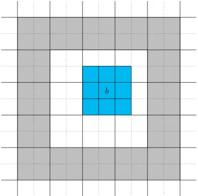
parent and the other one is from the interaction list of boxb. Figure 2.1 shows the interaction list in
two dimension. For each boxbat a given level, it will associate with five lists of boxes with different
b
Figure 2.1: Blue boxes are colleagues of boxband white boxes are the interaction list of b.
sizes. The definitions of these lists are as below:
List 1of box bdenoted byUb:
• Ifb is a parent box,Ub is empty;
• Ifb is a leaf box, Ub is composed of all the childless boxes adjacent to b and box b.
List 2of box bdenoted byVb:
• It consists of all boxes in the interaction list. i.e. all the children of the colleagues ofb’s
parent that are well separated fromb.
List 3of box bdenoted byWb:
• If b is a parent box,Wb is empty;
• If b is a leaf box,Wb consists of all descendant ofb’s colleagues whose parents are adjacent
tobbut not adjacent tobthemselves. Each box win Wb is separated frombby a distance
no less than the length of the side ofw.
List 4of box bdenoted byXb
• It is composed of all boxes csuch thatb2Wc.
• All boxes inXb are childless and larger thanb.
List 5of box bdenoted byYb
• It is formed by all boxes that are well-separated from b’s parent.
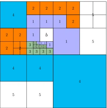
Figure 2.1 shows the associated five lists of box b. To reduce the huge factor in front ofO(N) of the original FMM, the new version of FMM introduced plane wave based translation operators to diagonalize the multipole-to-local translations from box b to its interaction list boxes. The
interaction list of box bwill be partitioned into six lists associated with the six coordinate directions
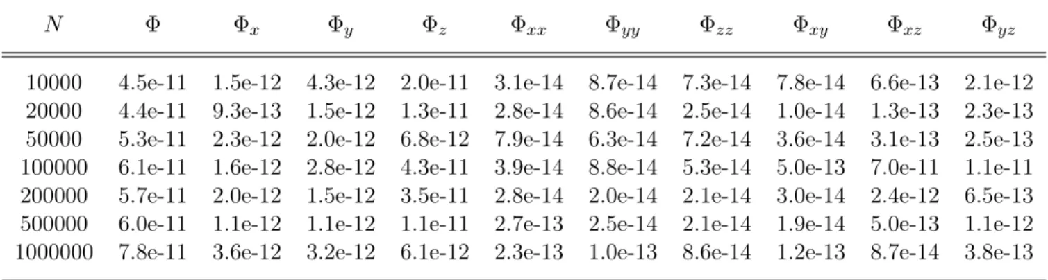
(+z, z,+y, y,+x, x) in three-dimensional space. Corresponding directions and the definitions of the directional lists are as below and Figure 2.1 shows the uplist of b.
• +zdirection is referred to asup. TheUplist for a boxbis formed of the boxes in the interaction
list which lie aboveb and are separated by at least one box in the +z direction.
• z direction is referred to as down. The Downlist for a box b consists of the boxes in the
1
1 1 1
1 1
1 1 1
2 2
2 2
2 2 2 2
2
3
3 3 3 3
3 3 3 3 3
4
4 4
4
5 5
5 5
b
Figure 2.2: Boxband its associated lists in two dimension
• +y direction is referred to as north. The Northlist for a box b consists of the boxes in the
interaction list which lie north ofb. They are separated by at least one box in the+y direction,
and are not contained in the Up, Down lists.
• y direction is referred to as south. The Southlist for a box b consists of the boxes in the
interaction list which lie south ofb. They are separated by at least one box in the y direction,
and are not contained in the Up, Down lists.
• +x direction is referred to as east. The Eastlist for a box b consists of the boxes in the
interaction list which lie east ofb. They are separated by at least one box in the +xdirection
and are not contained in the Up, Down, South, North lists.
• x direction is referred to as west. The Westlist for a box b consists of the boxes in the
interaction list which lie south ofb. They are separated by at least one box in the xdirection
and are not contained in the Up, Down, South, North lists.
Figure 2.3: The uplist of Boxb [2]
2.2 Approximation and Translation
2.2.1 Mathematical Preliminaries
The spherical harmonics Ynm(✓, ) are the angular portions of the solution to Laplace equation in spherical coordinates. The definition of spherical harmonics of degreenand order min [1] is as
below;
Ynm(✓,') =
r
2n+ 1 4⇡
s
(n |m|) (n+|m|)P
|m|
n (cos✓)eim',8n 0,|m|n (2.5)
Here,Pm
n are the associated Legendre functions which can be defined by the Rodrigues’s formula
Pnm(x) = ( 1)m(1 x2)m/2 d
m
dxmPn(x), (2.6)
wherePn(x) denotes the Legendre polynomial of degreenand satisfies
Pnm = ( 1)m(n m)! (n+m)!P
All together this gives Y m
n = ( 1)m(Ynm)⇤,8n 0,0mn.
A different definition of spherical harmonics in quantum physics is expressed as :
¯
Ynm(✓,') =
r
2n+ 1 4⇡
s
(n m) (n+m)P
m
n (cos✓)eim',8n 0,0mn. (2.7)
When 0mn, there is Y¯n m= ( ¯Ynm)⇤.
For a given value of n, there are2n+ 1 independent solutions of this form, one for each integer
m with n m n. The restrictions of n and |m| to non-negative integers with |m| n is a
consequence of the requirement thatPm
n should be non-singular at cos✓= ±1.
The Lemma 1 will be used for the computation of the field and the electric field gradient.
Lemma 1. (Properties of Spherical harmonics) For any n 0,0mn, there are
Ynm = Y¯nm (2.8)
Yn m = ( 1)mY¯n m. (2.9)
Derivatives As in [72], define the sphercal tensor operators
r0=@z,r+ =
1 p
2( @ @x+i
@
@y),r =
1 p
2( @ @x i
@
@y) (2.10)
there are
@ @x =
1 p
2(r+ r ), (2.11)
@ @y =
i
p
2(r++r ), (2.12)
@
@z = r0. (2.13)
Lemma 2. If f(r) is a function about r, and Y¯nm is the spherical harmonic function defined by 2.7,
8n 1,|m|n, and define
↵(n, m) =
s
(n+m)(n m)
(2n+ 1)(2n 1), ±(n, m) =
s
(n⌥m 1)(n⌥m)
2(2n 1)(2n+ 1) , (2.14)
there are
r0[f(r) ¯Ynm] =↵(n+ 1, m)(
df dr
n rf) ¯Y
m n+1
+↵(n, m)(df
dr + n+ 1
r f) ¯Y
m n 1,
(2.15)
r±[f(r) ¯Ynm] = ⌥(n+ 2, m)(df
dr n rf) ¯Y
m±1
n+1
+ ±(n, m)(df
dr+ n+ 1
r f) ¯Y
m±1
n 1 .
(2.16)
Proof. The details of the proof can be reached at [72].
Lemma 3. (Properties) Suppose for anyn 1,|m|n, ↵(n, m), (n, m) are defined as 2.14, there are
↵(n, m) = ↵(n, m), (2.17)
+(n, m) = (n, m). (2.18)
Apply Theorem 2 tof(r) =rn, there are
Corollary 1. If f(r) =rn, n 1, Ynm is defined by Equation (2.5), there are
r0[rnYnm] = (2n+ 1)↵(n, m)rn 1Ynm1,8n 1,|m|n, (2.19)
r±[rnYnm] = (2n+ 1) ±(n, m)rn 1Ynm±11,8n 1,|m|n. (2.20)
Lemma 4. Let f, g be real functions whose derivative exists at every point, there is
(r+)(f+ig) = [r (f ig)]⇤. (2.21)
For spherical harmonics defined by Equation (2.5), combine Lemma 3 and Lemma 4, the following theorem for spherical harmonics can be derived.
Theorem 2.2.1. The corresponding derivatives of spherical harmonics defined by Equation (2.5) are as below:
r+[rnYnm] = 8 > < > :
(2n+ 1) +(n, m)rn 1Ynm+11 8n 1,0mn;
(2n+ 1) +(n, m)rn 1Ynm+11 8n 1, nm 1;
(2.23)
r [rnYnm] =
8 > < > :
(2n+ 1) (n, m)rn 1Ynm11 8n 0,1mn; (2n+ 1) (n, m)rn 1Ynm11 8n 0, nm0.
(2.24)
2.2.2 Approximation Operators
All hierarchical N-body algorithms are based on the idea of evaluating combined effect of a set of distant particles instead of treating them individually. In this chapter, the Laplace kernel will be used as an example to present how the fast multipole methods extract, condense and transmit information on the adaptive Oct-tree structures. Two expansions operators including the multipole expansion and the local expansion, are fundamental in FMM. The multipole expansions allow one to group a cluster of particles that lie close together and treat them as if they are a single source. The local expansions transfer information from long range to near range. The proof of the theorems will be neglected. Interested readers can refer to [2] [66] for details.
Theorem 2.2.2 (Multipole Expansion). Suppose N particles with charges {qi}Ni=1 and positions {xi = (⇢i,↵i, i)}Ni=1 are located in a box centered at the origin. Then for any pointx= (r,✓, )2R3
outside the box, the potential (x) is given by
(x) =
1
X
n=0
n X
m= n
Mnm rn+1 ·Y
m
n (✓, ), (2.25)
where the multipole expansion coefficients Mnm are given by
Mnm=
N X
i=1
qi·⇢ni ·Yn m(↵i, i). (2.26)
Furthermore, for any p 1,
(x)
p X
n=0
n X
m= n
Mm
n
rn+1 ·Y
m
n (✓, ) PN
i=1|qi|
where ais the radius of the smallest sphere enclosing the box.
The above theorem describes an efficient representation of the far field potential due to a collection of sources. TSM means source-to-multipole operator andTLT is the local-to-target operator.
Theorem 2.2.3 (Local Expansion). Suppose N particles with charges {qi}Ni=1 and positions {xi=
(⇢i,↵i, i)}Ni=1 are located outside the sphere Sa of radius a centered at the origin. Then for any
point with coordinates x= (r,✓, )2Sa outside the box, the potential (x) generated by the charges
q1, q2, . . . , qN is described by the local expansion
(x) =
1
X
j=0
j X
k= j
Lkj ·Yjk(✓, )·rj, (2.27)
where the local expansion coefficients Lk
j are given by
Lkj =
N X
l=1 ql·
Yj k(↵l, l)
⇢jl+1 . (2.28)
Furthermore, for any p 1,
(x)
p X
j=0
j X
k= j
Lkj ·Yjk(✓, )·rj+1
PN i=1|qi|
a r
!⇣
r a
⌘p+1 .
2.2.3 Translation Operators
To form multipole expansions for all level of boxes, the FMM applies a divide-and-conquer strategy to collect the compressed information through merging and shifting its children’s multipole expansions for each parent box level by level. The following multipole-to-multipole translation operator TM M is applied in an upward pass for forming all the multipole expansions.
Theorem 2.2.4 (Translation of a Multipole ExpansionTM M). Suppose N particles with charges
{qi}Ni=1 and positions {xi= (⇢i,↵i, i)}Ni=1 are located in a sphereD centered atx0 = (⇢,↵, ). Then
for any point x= (r,✓, )2R3\D, the potential generated by the charges {q
i}Ni=1 is given by
(x) =
1
X Xn
Onm
where (r0,✓0, 0) are the spherical coordinates of the vector x x0.
Then for any point x= (⇢,✓, ) outside a sphere D1 with radius a+⇢ centered at the origin,
(x) =
1
X
j=0
j X
k= j
Mjk rj+1 ·Y
k j (✓, ),
where
Mjk=
j X
n=0
n X
m= n
Ok mj n ·i|k| |m| |k m|·Anm·Ak mj n ·⇢n·Yn m(↵, )
Ak j
, (2.30)
with Amn defined by the formula
Amn = ( 1)
n p
(n m)!·(n+m)!. (2.31)
Furthermore for any p 1,
(x)
p X
j=0
j X
k= j
Mk j
rj+1 ·Y
k
j (✓, )
PN i=1|qi|
r (a+⇢)
! ✓
a+⇢
r
◆p+1 .
The linear operator defined by Equation (2.29) converts the old multipole expansion coefficients
Ojk into the new multipole expansion Mjk and will denoted by TM M. The above theorem can be
used to obtain all multipole expansions from the finest level of boxes to the coarsest level in the upward pass.
In the downward pass from the coarsest refinement level to the finest level, local-to-local translation operatorTLL is carried out firstly to shift the parent box’s local expansion which contains the far-field
particle contributions into the center of the children’s boxes.
Theorem 2.2.5 (Translation of a Local expansion TLL). Consider a point x= (⇢,✓, ) in a box
centered atx0= (⇢,↵, ). The spherical coordinates of the vectorx x0 is(⇢0,✓0, 0). The pthorder local expansion of its parent box is described by
(x) =
p X
n=0
n X
m= n
Omn ·Ynm(✓0, 0)·r0n. (2.32)
Then the local expansion of that box is
(x) =
p X
j=0
j X
k= j
Lkj ·Yjk(✓, )·rj, (2.33)
where
Lkj =
p X
n=j n X
m= n
Omn ·i|m| |m k| |k|·An jm k·Akj ·Yn jm k(↵, )·⇢n j ( 1)n+jAm
n
, (2.34)
with Amn defined by (2.31).
After the local-to-local expansions in the downward pass, a box chas inherited information from
its parent box b. The second step for box c is trying to collect information from its interaction
list. Since all boxes in the interaction list are well-separated from c, a multipole-to-local expansion
operator TM L is applied to approximate the contribution from the interaction list of c instead of
communicating with each particle in this region.
Theorem 2.2.6 (Conversion of a Multipole Expansion into a Local expansion TM L). Suppose `
charges of strengths {qi}`i=1 are located inside a sphere Dx0 centered at x0 = (⇢,↵, ) with radius
a, and⇢>(c+ 1)afor some constant c >1. Then the corresponding multipole expansion given by (2.25) converges inside another sphere D0 with radius acentered at the origin. For any point x2D0
with spherical coordinates (r,✓, ), its potential due to charges inside Dx0 is described by
(x) =
1
X
j=0
j X
k= j
Lkj ·Yjk(✓, )·rj, (2.35)
where
Lkj =
1
X
n=0
n X
m= n
Onm·i|k m| |k| |m|·Amn ·Akj ·Ynm k+j (↵, )
( 1)nAm k
n+j ·⇢j+n+1
. (2.36)
Furthermore, for any p 1,
(x)
p X
j=0
j X
k= j
Lkj ·Yjk(✓, )·rj+1
PN i=1|qi|
ca a ! ✓ 1 c ◆p+1 . (2.37)
In all of the above expansions, the multipole-to-local expansion is the bottleneck and the complexity is O(p4) if the expansions are approximated with p2 terms for each box. In three
dimensions, a given box could have up to189boxes in its interaction list. As a result, in the original FMM method, the multipole-to-local expansion for a given box could cost 189p4 operations which
makes it not practical especially for large-scale problems.
To make the original fast multipole method more promising, a new version of FMM [1] based on a new diagonal form for translation operators was introduced to produce high accuracy at an acceptable computation cost. Interested readers can also refer to [73],[74], and [75] for other version translation operators. Here, the plane-wave expansion with exponential basis [2] will be presented to diagonalize the TM L operator. In three dimension, six plane-wave expansions for direction
(+z, z,+y, y,+x, x) are introduced and the multipole-to-local translator has been decomposed intoTM L =TEL TEE TM E, where TM E is the multipole-to-exponential operator, TEE represented
the exponential-to-exponential operator, andTEL denoted as the exponential-to-local operator. This
decomposition will reduce the cost from 189p4 to6p3+ 189p2 for each box. If the merge and shift
strategy is applied, the cost for multipole to local expansion will be6p3+ 40p2 and this result could
be further improved to 15p2logp+ 40p2 by applying FFT.
In the new version of FMM, the interaction list of a given box chas been subdivided into Uplist,
Downlist, Eastlist, Westlist, Northlist, and Southlist. These six lists are corresponding to directions
(+z, z,+y, y,+x, x). For any box c in the six interaction lists of b, the multipole expansion
centered inbwill be firstly translated into an exponential expansion about a center of a box, then
shift it using exponential-to-exponential expansion to a new center of an interaction list box. Once the exponential expansions from the interaction list boxes have been collected, the exponential expansions will be translated to a local expansion in boxc using exponential-to-local operator.
The translations of upward (+z) direction are illustrated here and translations for the other directions can be processed similarly.
Theorem 2.2.7 (Multipole Expansion to Exponential expansionTM E). Suppose box b containing
N charges{qi, i= 1, . . . , N} is centered at the origin and with unit volume. The charges are located
at points {xi= (xi, yi, zi)}. Let x be the location of a particle in box c andc2 Uplist(b). Given the
multipole expansion of (x) as
(x) =
1
X
n=0
n X
m= n
Mnm rn+1 ·Y
m
n (✓, ). (2.38)
Then
(x)
s(✏)
X
k=1
MX(k)
j=1
W(k, j)e kzei k(xcos↵j+ysin↵j) < A✏, (2.39)
and
W(k, j) = !k
M(k)
1
X
m= 1
( i)|m|eimaj
1
X
n=|m|
Mnm
p
(n m)!(n+m)!
n
k, (2.40)
where A = PNi=1|qi|, { k,!k} are the quadrature nodes and weights returned by the generalized
Gaussian quadrature. s(✏) denotes the number of k’s for accuracy requirement✏. For each k, M(k)
denotes the number of quadrature needed for the trapezoid rule. And↵j = 2M⇡kj.
TM E maps the multipole expansion coefficients {Mnm)}, n = 0, . . . , p, m = n, . . . , n to the
corresponding exponential expansion coefficients {W(k, j)}.
Theorem 2.2.8 (Exponential to Exponential expansion TEE). Suppose box b containing N charges
{qi, i= 1, . . . , N} is centered at the origin and with unit volume. The charges are located at points
{xi = (xi, yi, zi)}. Let x be the location of a particle in box c. c is a box in Uplist(b) and centered at
(x1, y1, z1). Given the exponential expansion centered at the origin of (x) as
(x) =
s(✏)
X
k=1
MX(k)
j=1
W(k, j)e kzei k(xcos↵j+ysin↵j)+O(✏), (2.41)
then
(x) =
s(✏)
X
k=1
MX(k)
j=1
V(k, j)e k(z z1)ei k((x x1) cos↵j+(y y1) sin↵j)+O(✏), (2.42)
where
V(k, j) =W(k, j)e kz1ei k(x1cos↵j+y1sin↵j). (2.43)
The exponential-to-exponential operator maps the original set of exponential expansion coefficients
Theorem 2.2.9 (Exponential expansion to Local expansion TEL). Suppose box b containing N
charges {qi, i= 1, . . . , N} is centered at the origin and with unit volume. The charges are located at
points {xi = (xi, yi, zi)}. Letx be the location of a particle in boxc and c2 UPlist(b). Given the
exponential expansion of (x) as
(x)
s(✏)
X
k=1
MX(k)
j=1
W(k, j)e kzei k(xcos↵j+ysin↵j) < A✏, (2.44)
where A=PNi=1|qi|, { k,!k}. Then
(x)
1
X
n=0
n X
m= n
Lmn ·Ynm(✓, )·rn < A✏, (2.45)
where
Lmn = ( i)|
m|
p
(n m)!(n+m)!
s(✏)
X
k=1
( k)n MX(k)
j=1
W(k, j)eim↵j. (2.46)
Translation operatorTEL maps the shifted set of exponential expansion coefficients {W(k, j)} to
the corresponding truncated harmonic expansion coefficients {Lmn}, n= 0, . . . , p, m= n, . . . , n.
2.3 Local Expansions of the Fields and Electric Field Gradients
This section will start with how to use the local expansion coefficients of the far-field potential to derive the far-field part of the fields and the electric field gradients. Next the function of computing the electric field gradients using FMM is added for existing FMM solver. The near-field calculations will be directly evaluated and the details will be omitted here.
2.3.1 Electrostatic Fields
Lemma 5. Consider a pointx= (r,✓, )outside a box centered at the origin. There are N particles
with charges {qj}Nj=1 and locations{xj = (⇢j,↵j, j)}Nj=1 in the box, the pthorder local expansion of
the potential atx is described by
(x) =
p X
`=0
`
X
m= `
Lm` ·Y`m(✓, )·r`. (2.47)
Here, Lm
` is the local expansion coefficients given by
Lm` =
N X
j=1 qj·
Y` m(↵j, j)
⇢`j+1 . (2.48)
So L`m = (Lm
` )⇤. Define the notations below for all 0`p 1,|m|`,
D0(`, m) = (2`+ 3)↵(`+ 1, m)Lm`+1Y`mr`, (2.49)
Dp(`, m) = (2`+ 3) +(`+ 1, m 1)Lm`+11Ylmr`,
Dm(`, m) = (2`+ 3) (`+ 1, m+ 1)Lm`+1+1Ylmr`,
thepth order local expansion of the potential under spherical tensor operators at x is described by
r0( ) =
p 1
X
`=0
D0(`,0) +
p 1 X `=1 ` X m=1
2<(D0(`, m)), (2.50)
r+[ ] =
p 1
X
`=0
" 0 X
m= ` `
X
m=1
#
Dp(`, m), (2.51)
r [ ] =
p 1
X
`=0
" 1 X
m= ` `
X
m=0
#
Dm(`, m). (2.52)
Proof.
r0( ) =
p X
`=0
`
X
m= `
Lm` r0(r`Y`m)
= p X `=1 ` 1 X
m= (` 1)
Lm` ↵(`, m)(2`+ 1)r` 1Y`m1.(0|m|` 1
(2.53)
Let`0 =` 1and change back the index from `0 to`.
r0( ) =
p 1
X
`=0
`
X
m= `
Lm`+1↵(`+ 1, m)(2`+ 3)r`Y`m
=
p 1
X
`=0
(2`+ 3)↵(`+ 1,0)L0`+1Y`0r`
+
p 1
XX`
2(2`+ 3)↵(`+ 1, m)<(L`m+1Y`m)r`.
r+( ) = p X `=0 ` X
m= `
Lm` r+(r`Y`m)
= p X `=1 1 X
m= (` 1)
Lm` +(`, m)(2`+ 1)r` 1Y`m+11
+ p X `=1 ` 1 X m=0
Lm` ( +(`, m))(2`+ 1)r` 1Y`m+11 .
(2.55)
Let`0 =` 1, m0 =m+ 1, and change back index to`, m, the theorem can be derived easily. Similar
procedure could be applied to r ( ).
Theorem 2.3.1. [Electronic Fields of the far-field Part] Thepthorder local expansion of electrostatic
fields ( @@x, @@y, @@z) due to the charges located in boxes well separated from box b can be evaluated
as below
@ @x =
p 2
"p 1 X
`=1
`
X
m=1
<(Dp(`, m)) p 1 X `=0 ` X m=0
<(Dm(`, m) #
, (2.56)
@ @y =
p 2
"p 1 X
`=1
`
X
m=1
=(Dp(`, m)) p 1 X `=0 ` X m=0
=(Dm(`, m) #
, (2.57)
@ @z =
p 1
X
`=0
D0(`,0) +
p 1 X `=1 ` X m=1
2<(D0(`, m)). (2.58)
Proof. Note that
Dp(`, m) =Dm(`, m)⇤, (2.59)
D0(`, m) =D0(`, m)⇤. (2.60)
According to Lemma 5, the pthorder of local expansions of the partial derivatives of potential
can be derived from
@ @x =
1 p 2 p 1 X `=0 " ` X m=0
(Dp(`, m) +Dm(`, m))
`
X
m=1
(Dp(`, m) +Dm(`, m)) #
= p1 2 p 1 X `=0 " ` X m=0
2<(Dm(`, m)) +
`
X
m=1
2<(Dp(`, m)) #
. (2.61)
Follow the same procedure to get the proof of Equation (2.57) and Equation (2.58).
2.3.2 The far-field Electric Field Gradients Corollary 2. For 8` 1,|m|`, there are
r2+[rlY`m] = (2l 1)(2l+ 1) +(`, m) +(` 1, m+ 1)r` 2Y`m+22 ,
r2[rlY`m] = (2l 1)(2l+ 1) (`, m) (` 1, m 1)r` 2Y`m22,
r20[rlY`m] = (2l 1)(2l+ 1)↵(`, m)↵(` 1, m)r` 2Y`m2,
r+r [rlY`m] = (2l 1)(2l+ 1) +(`, m) (` 1, m+ 1)r` 2Y`m2,
r+r0[rlY`m] = (2l 1)(2l+ 1)↵(`, m) +(` 1, m)r` 2Y`m+12 ,
r r0[rlY`m] = (2l 1)(2l+ 1)↵(`, m) (` 1, m)r` 2Y`m21. (2.62)
Proof. Apply Theorem 2.2.1 repeatedly to get the conclusions.
Theorem 2.3.2. Consider a point x= (r,✓, ) outside a box centered at the origin. There are N
particles with charges {qj}Nj=1 and locations {xj = (⇢j,↵j, j)}Nj=1 in the box, the pth order local
expansion of the potential at x is described by
(x) =
p X
`=0
`
X
m= `
Lm` ·Y`m(✓, )·r`. (2.63)
Here, Lm
` is the local expansion coefficients given by
Lm` =
N X
j=1 qj·
Y` m(↵j, j)
Define the notations below:
Dpp(`, m) = (2`+ 3)(2`+ 5) +(`+ 2, m 2) +(`+ 1, m 1)r`Lm`+22Y`m,
Dmm(`, m) = (2`+ 3)(2`+ 5) (`+ 2, m+ 2) (`+ 1, m+ 1)r`Lm`+2+2Y`m,
Dpm(`, m) = (2`+ 3)(2`+ 5) +(`+ 2, m) (`+ 1, m+ 1)r`Lm`+2Y`m,
Dmp(`, m) = (2`+ 3)(2`+ 5) (`+ 2, m) +(`+ 1, m 1)r`Lm`+2Y`m,
D00(`, m) = (2`+ 3)(2`+ 5)↵(`+ 2, m)↵(`+ 1, m)r`Lm`+2Y`m,
Dp0(`, m) = (2`+ 3)(2`+ 5)↵(`+ 2, m 1) +(`+ 1, m 1)r`Lm`+21Y`m,
Dm0(`, m) = (2`+ 3)(2`+ 5)↵(`+ 2, m+ 1) (`+ 1, m+ 1)r`Lm`+2+1Y`m.
Then the pthorder local expansions of the second order derivatives of the potential at xis
@2
@x2 =
p 2 X `=0 " ` X m=2
<(Dpp(`, m)) +
`
X
m=0
<(Dmm(`, m)) <(Dpp(`,1)) # p 2 X `=0 " ` X m=0
Dpm(`, m) +
`
X
m=1
Dmp(`, m) #
, (2.65)
@2 @y2 =
p 2 X `=0 " ` X m=2
<(Dpp(`, m)) +
`
X
m=0
<(Dmm(`, m)) <(Dpp(`,1)) # p 2 X `=0 " ` X m=0
Dpm(`, m) +
`
X
m=1
Dmp(`, m) #
, (2.66)
@2
@z2 =
p 2 X `=0 " ` X m=1
2<(D00(`, m)) +D00(`,0)
#
, (2.67)
@2 @x@y =
p 2 X `=0 " ` X m=2
=(Dpp(`, m))
`
X
m=0
=(Dmm(`, m)) =(Dpp(`,1)) #
, (2.68)
@2 @x@z =
p 2 p 2 X `=0 " ` X m=1
<(Dp0(`, m))
`
X
m=0
<(Dm0(`, m))
#
, (2.69)
@2
@y@z =
p 2 p 2 X `=0 " ` X m=1
=(Dp0(`, m))
`
X
m=0
=(Dm0(`, m))
#
. (2.70)
![Figure 2.3: The uplist of Box b [2]](https://thumb-us.123doks.com/thumbv2/123dok_us/8305185.2199650/31.918.170.716.129.450/figure-the-uplist-of-box-b.webp)