APPLICATIONS OF GENERALIZED FIDUCIAL INFERENCE IN HIGH FREQUENCY DATA
Dimitris Katsoridas
A dissertation submitted to the faculty of the University of North Carolina at Chapel Hill in partial fulfillment of the requirements for the degree of Doctor of
Philosophy in the Department of Economics.
Chapel Hill 2015
c
ABSTRACT
DIMITRIS KATSORIDAS: Applications of Generalized Fiducial Inference in High Frequency Data
(Under the direction of Jan Hannig)
Fiducial inference was introduced by R.A. Fisher Fisher (1930) as a response to the Bayesian approach to inference. The Bayesian paradigm begins by assuming a prior
dis-tribution on the parameter space and inference is conducted via the posterior disdis-tribution.
Fisher, however, was concerned about the choice of the prior distribution, especially when
there is insufficient information about the parameters of interest. To overcome this weakness,
Fisher introduced the fiducial argument which is based on the following idea: randomness
is transferred from the model space to the parameter space and a distribution on the
pa-rameter space can is defined that captures all of the information the data contains about
these parameters. Fisher’s idea, however, soon fell into disfavor since some of the properties Fisher claimed did not hold.
Recently, Fisher’s inferential framework was revived through its connection to
general-ized inference. Hannig (2009) generalgeneral-ized Fisher’s idea and introduced a framework where
fiducial distributions can be defined properly. The main topic of this dissertation is to apply
generalized fiducial inference methods to study intraday volatility using high frequency stock
market data. In particular, we apply a generalized fiducial framework that is designed for
interval data to study high frequency volatility, Hannig (2013). Our approach allows us to
view the bid-ask spread as a natural interval around the latent price and use high frequency
quotes for estimation. Modeling the spread in this manner allows us to take advantage of the features of the observed prices inherent to the trading process, such as rounding, and
reduce the impact microstructure frictions cause to estimation. We demonstrate that our
approach is very effective in estimating volatility and outperforms all alternative
of microstructure frictions. In chapter 3, we extend our framework to allow for additive
components. In the final chapter, we perform an empirical study to compare alternative
realized volatility estimators through option pricing formulas. We find that the choice of
ACKNOWLEDGEMENTS
I take this opportunity to express gratitude to my advisor, Professor Jan Hannig. His passion about research, his encouragement and his generosity has been a tremendous
in-spiration for me. Without his guidance and support this dissertation would not have been
possible.
I would like to thank Professors Jonathan Hill, Shankar Bhamidi, Ju Hyun Kim and
Valentin Verdier for their support and participation on my dissertation committee.
Finally, I would like to thank my family and Marianna Feretzaki for their endless love
TABLE OF CONTENTS
LIST OF TABLES . . . ix
LIST OF FIGURES . . . xi
1 Introduction . . . 1
1.1 Thesis overview . . . 1
1.2 Generalized Fiducial Inference . . . 1
1.3 Volatility Estimation and Microstructure Noise . . . 5
1.3.1 Quasi Maximum Likelihood Estimation . . . 8
1.3.2 Pre-averaging Approach . . . 9
1.3.3 Realized Kernels . . . 11
1.3.4 Two-Scales and Multi-Scales Realized Volatility . . . 12
1.4 Sequential Monte Carlo (SMC) methods . . . 16
2 Generalized Fiducial Inference for High Frequency Data in the Presence of Rounging Errors . . . 19
2.1 Summary . . . 19
2.2 Introduction . . . 19
2.3 Generalized Fiducial Inference for HF data . . . 23
2.4 Estimation Method . . . 24
2.4.1 Sequential Monte Carlo Algorithm . . . 24
2.4.2 Resampling - Alteration Step . . . 27
2.5 Theoretical Results . . . 28
2.5.1 Preliminaries - Likelihood of Exact Data . . . 28
2.5.2 Likelihood of Rounded Data . . . 30
2.5.4 Generalized Fiducial Density . . . 33
2.5.5 Bernstein-von Mises theorem . . . 35
2.5.6 Proofs and Auxiliary Results . . . 41
2.6 Combinations of Fiducial Distributions . . . 44
2.7 Simulation and Robustness checks . . . 46
2.7.1 Constant Volatility . . . 48
2.7.2 Stochastic Volatility . . . 54
2.8 Empirical Study . . . 54
2.8.1 Illustration . . . 59
2.8.2 Time varying spread . . . 61
2.9 Conclusion . . . 63
3 Generalized Fiducial Inference for High Frequency Data in the Presence of Presence of Rounging and Additive Errors . . . 64
3.1 Summary . . . 64
3.2 Introduction . . . 64
3.3 Generalized Fiducial Inference for HF data . . . 67
3.4 Estimation . . . 69
3.4.1 The SMC Algorithm . . . 69
3.4.2 Resampling - Alteration Step . . . 73
3.4.3 Convergence of the Algorithm . . . 76
3.5 Combinations of Fiducial Distributions . . . 84
3.6 Simulation and Robustness checks . . . 85
3.6.1 Comparison with the MLE . . . 89
3.6.2 Stochastic Volatility . . . 91
3.7 Empirical Study . . . 95
3.7.1 Analysis of Alcoa Inc. on May 4, 2007 . . . 95
3.7.2 Time varying spread . . . 98
4 Option Pricing with Alternative Realized Volatility Estimators . . . 101
4.1 Summary . . . 101
4.2 Introduction . . . 101
4.3 The GARV Model . . . 105
4.4 Option Pricing . . . 106
4.4.1 Risk neutralization . . . 106
4.4.2 Option Pricing . . . 110
4.5 Data, Methodology and Results . . . 110
4.5.1 Data . . . 110
4.5.2 Methodology . . . 111
4.5.3 Results . . . 114
A Simulation Results for Chapter 2 . . . 117
B Simulation Results for Chapter 3 . . . 124
C Data Cleaning Filters . . . 132
D Moment generating functions for the GARV model . . . 133
LIST OF TABLES
2.1 Performance of the combined fiducial distribution estimator under
constant volatility. . . 49
2.2 Performance of the block fiducial distribution estimator under
con-stant volatility. . . 50
2.3 Performance of the combined fiducial distribution estimator under
constant volatility and different intensity levels. . . 52
2.4 Performance of the block fiducial distribution estimator under
con-stant volatility and different intensity levels. . . 53
2.5 Performance of the combined fiducial distribution estimator under
stochastic volatility. . . 55
2.6 Performance of the block fiducial distribution estimator under
stochastic volatility. . . 56
2.7 Performance of the combined fiducial distribution estimator under
stochastic volatility and different intensity levels. . . 57
2.8 Performance of the block fiducial distribution estimator under
stochastic volatility and different intensity levels. . . 58
3.1 Empirical coverage of the parameters. Block distributions . . . 87
3.2 Performance of the daily block point estimator . . . 88
3.3 Empirical coverage of the parameters as the intensity of the arrival
times becomes larger. Block distributions . . . 89
3.4 Performance of the daily fiducial block point estimator as the
inten-sity of the arrival times becomes large. . . 90
3.5 Performance the daily block point estimator as the block size increases. . . 91
3.6 Performance of the daily combined fiducial point estimator against
the MLE. Starting price isS0 = 10. . . 92 3.7 Performance of the daily combined fiducial point estimator against
the MLE. Starting price isS0 = 20. . . 92 3.8 Performance of the daily combined fiducial point estimator against
the MLE. Starting price isS0 = 30. . . 93 3.9 Performance of the daily combined fiducial point estimator against
3.10 Performance of the daily combined fiducial point estimator against
the MLE when volatility is stochastic. Starting price isS0 = 10. . . 94 3.11 Summary statistics for the combined distributions for Alcoa Inc. . . 96
3.12 Summary statistics for the first block distributions for Alcoa Inc.
(AA) on May 4, 2007, before and after the quote revision . . . 99
4.1 SNP500 Index Option Data 2000-2007. . . 112
LIST OF FIGURES
1.1 Illustration of the sampling scheme . . . 5
2.1 Combination of block distributions. . . 46
2.2 Rounding issues . . . 51
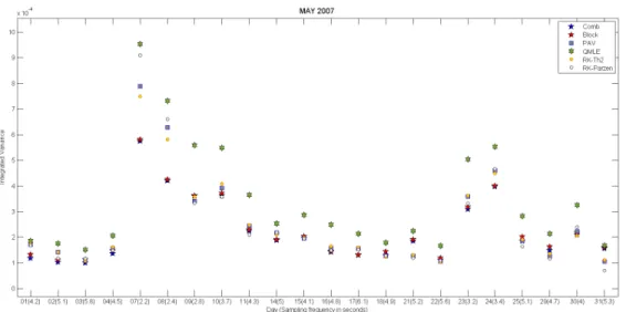
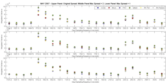
2.3 Alcoa Inc. (AA) on May4, 2007. . . 60
2.4 Volatility Estimates for Alcoa Inc. (AA) on May 2007. . . 60
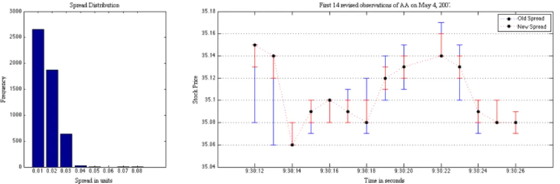
2.5 Spread distribution and revised quotes of Alcoa Inc. . . 61
2.6 Revised Volatility Estimates of Alcoa Inc. . . 62
3.1 Illustration of the fiducial methodology. . . 69
3.2 Practical illustration of the sapling scheme. . . 73
3.3 Alcoa Inc. (AA) on May4, 2007 . . . 95
3.4 Fiducial densities for Alcoa Inc. . . 96
3.5 Volatility and noise estimates for Alcoa Inc. . . 97
3.6 Volatility and noise signature plots for Alcoa Inc. . . 98
CHAPTER 1
Introduction
1.1 Thesis overview
In this thesis, there are main three contributions divided in three chapters. In chapter 2, we apply a generalized fiducial framework that is designed for interval data to study high
frequency volatility. We assume that the only source of microstructure noise is rounding
errors. In chapter 3, we extend our framework to allow for additive components. In the final
chapter, we perform an empirical study to compare alternative realized volatility estimators
through option pricing formulas. We find that the choice of volatility estimators does matter.
All supplementary material is included in the appendices.
1.2 Generalized Fiducial Inference
Fiducial inference was introduced by R.A. Fisher (Fisher, 1930) as a response to the Bayesian
approach to inference. The Bayesian paradigm begins by assuming a prior distribution on the
parameter space and inference is conducted via the posterior distribution. Fisher, however,
was concerned about the choice of the prior distribution, especially when there is insufficient
information about the parameters of interest. To overcome this weakness, Fisher introduced
the fiducial argument which is based on the following idea: randomness is transferred from
the model space to the parameter space and a distribution on the parameter space can
is defined that captures all of the information the data contains about these parameters. Subsequently, the fiducial distribution, which resembles the Bayesian posterior, can be used
for inference procedures such as parameter estimation and confidence sets.
As a simple illustration of the idea we consider the following example: Let y be a
the observed value y, the fiducial argument solves for the unknown parameter µ, that is,
µ=y−Z. Even though the actual value ofZ is unknown, its distribution is fully known and can be used to construct a distribution on the unknown parameter . This distribution on
is known as the fiducial distribution, which in this example is simply µvN(y,1). Hannig (2009) provides a solid introduction to the fiducial argument, together with facts about the
historical development of the idea.
Soon after its inception, fiducial inference fell into disrepute among statisticians since it
was shown that some of the properties Fisher claimed did not hold. In particular, not only
statistical procedures based on the fiducial argument were non-exact in the frequentist sense,
but also, there were non-uniqueness issues associated with the specification of these
proba-bility measures, see for example Lindley (1958) and Zabell (1992). Even though some recent
attempts were made to revive fiducial procedures (Fraser (1961a,b, 1966, 1968), Dempster
(1968), Dawid and Stone (1982), Barnard (1995)), it was until recently when Hannig et al.
(2006) connected fiducial inference to generalized inference, introduced by Tsui and
Weera-handi (1989). Tsui and WeeraWeera-handi (1989) performed hypothesis testing by introducing the concept of generalized p-values and Weerahandi (1993) constructed generalized confidence
intervals by introducing the notion of a generalized pivotal quantity, based on the former
idea of generalized p-values. Hannig et al. (2006) showed that most generalized pivotal
inference procedures are identical to procedures obtained using fiducial inference. In fact,
their recipe was introduced as a generalization of the idea of a generalized pivot.
The generalized fiducial argument expresses the dataXthrough a data generating equa-tion of the form
X=G(U, ξ) (1.2.1)
where G(,) is a jointly measurable structural equation based on the model under con-sideration, ξ ∈ Ξ are the parameters of interest, and U is the random component of the structural equation; a random vector whose distribution is completely known, independent
image of Gas follows
Q(x,u) ={ξ∈Ξ :x=G(u, ξ)} (1.2.2)
wherexis the observed data andu is a realization ofU.
The next step is to use the set function Q and define a distribution on the parameter space Ξ. The distribution of U will be used to draw samples of Q(x,u) given the data x. However, using equation 1.2.2 to define a fiducial distribution needs caution. There are three sources of non-uniqueness that may arise in this framework and one needs to address
them in order to define fiducial distributions properly. In particular, non-uniqueness can
occur ifQhas more than one element, ifQis empty, or due to the selection of the structural
equation.
In the case where there is more than one element in Q, non uniqueness can be resolved
by defining a rule, sayV, for selecting an element inQ. Therefore,V (Q(x,u))will be used to define the fiducial distribution. Discussion on how to select a rule can be found in Hannig
(2009). In the case where Q is empty, non-uniqueness can be resolved by conditioning on
the event {Q(x,U)6=∅}. This can be achieved by removing realizations of U for which there is no ξ solving equation x=G(u, ξ) and then re-normalizing the probabilities, i.e., use the distribution ofU conditional on the event {there is at least oneξ solving equation x=G(u, ξ)}. A generalized fiducial distribution for parameterξ is then defined as
V(Q(x,U∗))| {Q(x,U∗)6=∅} (1.2.3)
whereU∗ represents an independent copy of U.
A random element Rξ with distribution 1.2.3 is termed generalized fiducial quantity
(GFQ). Hannig (2009) showed that if the data generating equation 1.2.1 can be re-written
asXi=gi(U, ξ) for i= 1, . . . , n, implying that G= (g1, . . . , gn), then one can identify the
generalized fiducial density of Rξ. Assuming that the dimension of parameterξ isp, where
p≤n, we can define the following quantities. Leti= (i1, . . . , ip) denote a random selection
of indices from {1, . . . , n}. Let Xi = Xi1, . . . , Xip
and Ui = Ui1, . . . , Uip
denote the
and Gic denote the remaining components of X, U and G respectively. Then, assuming thatGi is invertible and differentiable with respect toUi, the generalized fiducial density is given by
fRξ(ξ) =
fX(x|ξ)J(x, ξ)
´
ΞfX(x|ξ 0
)J(x, ξ0)dξ0
where
J(x, ξ) =
n p
−1 X
i=(i1,...,ip)
det∂ξ∂ G−i1(yi, ξ)
det∂y∂
iG
−1 i (yi, ξ)
It should be clear that when the dimension of the parameter space is p, we can arbitrarily
select p equations to solve for ξ and condition the remaining n−p equations of G on the
solution of the first p.
From the discussion above, it is evident that the event{Q(x, U∗)6=∅}has zero probabil-ity only if the probabilprobabil-ity of generating the data{X=x} is zero. However, the probability of observing data coming from a continuous distribution is always zero and conditioning
on sets of probability zero may not be well defined (Borel paradox). This problem can be addressed by taking advantage of the fact that observed data have some degree of known
uncertainty. For example, most data-sets are discretized due to the resolution of the
in-strument that collects them, computers store discretized data due to memory limitations
and financial prices move in minimum increments (ticks). Using this “known” uncertainty,
we can create a small interval around the observed value set and replace the zero
proba-bility event {X=x} with the event {X∈Ax} where Ax contains the observed value x. Since Pξ(X∈AX)>0 the Borel paradox is resolved. Hannig (2013) presents the
general-ized fiducial inference framework for discretgeneral-ized data, pointing out that the nature of this data provide an attractive way to define generalized fiducial distributions, overcoming the
non-uniqueness due to Borel paradox.
A simple illustration on how discretized/interval data can be used in the context of
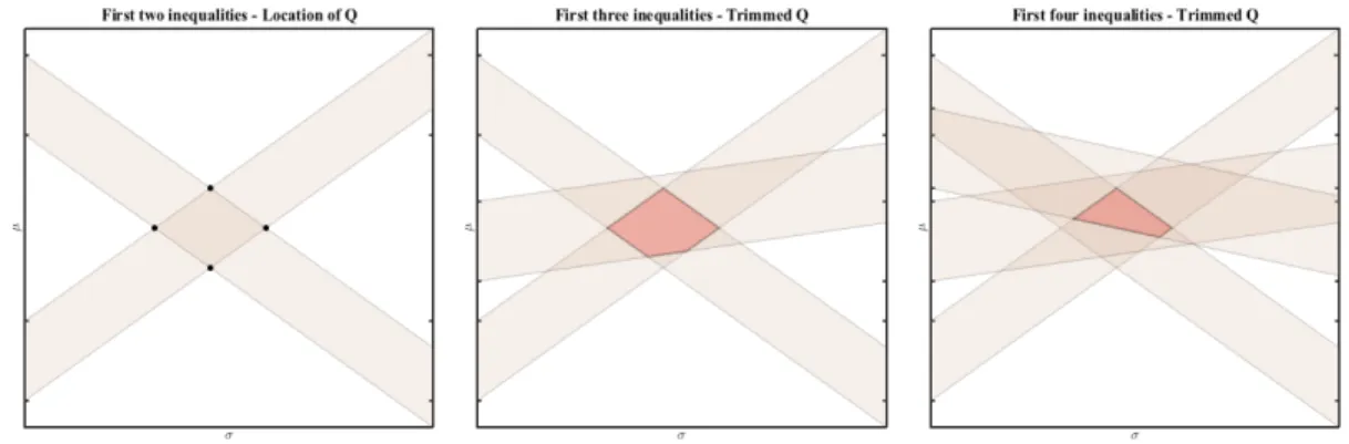
Figure 1.1: Illustration of the sampling scheme. The left panel illustrates how the first two inequalities can be used to generate Q, given that we generated z1 and z2 (with no restriction). The middle panel illustrates how the third inequality trims the polygon
Q, given that we generated z3 conditional on the first two inequalities. The right panel illustrates the update ofQ using the fourth inequality.
(y1, . . . , yn). In order to identify the setQ, equation 1.2.2, we can use the first two
inequali-ties1 and solve for the unknown parameters(µ, σ). This generates four pairs of(µ, σ), given that we generated z1 andz2 (with no restriction). The only requirement for this step is to havez1 6=z2, but we note thatP(Z1 6=Z2) = 1. Subsequently, we generatez3 such that the first three inequalities are satisfied and we update the set Q (a polygon in this setup) in a
way that all points(µ, σ)satisfy all inequalities. We repeat the same steps for all remaining inequalities. Finally, Picking randomly points(µ, σ) fromQ amounts to sampling from the fiducial distribution (2). Repeating the procedure several times generates a fiducial sample.
Figure 1.1 illustrates the sampling scheme for this simple model.
1.3 Volatility Estimation and Microstructure Noise
Estimating volatility using high frequency data (HFD) has been in the forefront of research
in financial econometrics. However, the enormous availability of HFD has been a blessing
and a curse to researchers since recorded prices are contaminated by market microstructure frictions. As a result, the maintained hypothesis that efficient prices are semimartingales
is not consistent with observed data. In fact, observed prices resemble semimartingales
1
recorded with error (MS noise).
In the standard microstructure setup, the efficient/unobserved log-price process, denoted
by Xt=log(St), is assumed to follow an Ito process:
Xt=X0+ ˆ t
0
µsds+
ˆ t
0
σsdWs
where Wt is a Brownian motion, µt is the drift of the process and σt is the
instan-taneous variance of the returns. Both µt and σt are adapted locally bounded
ran-dom processes. The process is assumed to evolve in [0, T] and is observed in the grid
Gn={0 =t0 < t1 < ... < tn=T}.The quantity of interest is integrated volatility over the
time period [0, T], namely,
hX, XiT = ˆ T
0
σt2dt
In the absence of market microstructure frictions, integrated volatility can be estimated
consistently with the so called “realized volatility” estimator. This estimator is nothing but
the quadratic variation relative to the gridGn. That is
[X, X]Gn
t = X
tj+1≤t
Xtj+1−Xtj
2 p
→[X, X]t=hX, Xit= ˆ t
0
σ2sds
However, microstructure noise is present and the estimator above is heavily biased. The
first remedy to MS noise was to use sparse samples. For example, Andersen et al. (2001)
showed that sampling every five minutes helps mitigate the effects of microstructure noise.
However, this amounts to discarding most the data available. For instance, if we have
available transaction records on a liquid stock traded once every second, then the sample
consists of 23,400 observations2. Therefore, if sampling takes place once every 5 minutes,
then - whether or not this is the optimal thing to do - it amounts to retaining only 78
observations. Stated differently, one is throwing away 299 out of every 300 transactions.
From a statistical perspective, this is unlikely to be the optimal solution, see Aït-Sahalia et al. (2005).
2
The first solution to MS noise was to assume that observed prices are the sum of the
effi-cient log-price and a stochastic component capturing all microstructure frictions. Typically,
the observed log-pricesYtmare assumed to be versions ofXtmunder the usual representation
Ytm =Xtm+Utm
whereUtm is introduced to capture a variety of frictions. These include frictions inherent in
the trading process, such as, bid–ask bounces and discreteness of price changes, as well as,
frictions attributed to informational effects, such as, differences in trade sizes, informational
content of price changes, gradual response of prices to a block trade, strategic component of the order flow and inventory control effects, see for example Aït-Sahalia et al. (2005).
Microstructure frictions are responible for most of the stylized facts of the high frequency
returns. For example, price discreteness leads to transaction changes of zero, 1 cent, 2 cents,
etc. which may result in a very small number of log-returns. As a result, log-returns
excibit high kurtosis (most tick-by-tick transactions equal their most recent transaction)
and temporal dependence. Moreover, bid-ask bounces3 bias upwards the variance of the
log-returns and cause negative first order autocorrelation, see for example Engle and Russell
(2004).
Estimation of volatility accounting for microstructure noise has been studied both
para-metrically and non-parapara-metrically. Parametric modeling includes the framework by
Aït-Sahalia et al. (2005) and Xiu (2010). Non-parametric modeling consists mainly of three
dif-ferent approaches. Zhang et al. (2005) and Zhang (2006) developed the Two-Scale (TSRV)
and Multi-Scale (MSRV) realized volatility estimators, Barndorff-Nielsen et al. (2008)
de-veloped the Realized Kernel (RK) volatility estimators and Podolskij and Vetter (2009) use
the pre-averaging method. Most of the aforementioned estimators were originally developed
on the assumption that noiseUtm is iid with mean zero and varianceσ
2
u, independent ofX.
Below, we discuss briefly the most commonly used approaches in this literature.
3Bid-ask bounces are attributed to price discreteness. Transactions occur either on the bid or the ask.
1.3.1 Quasi Maximum Likelihood Estimation
Following Aït-Sahalia et al. (2005), the process is assumed to evolve in [0, T] and is ob-served/quoted in the grid Gn = {0 =t0< t1< ... < tn=T}. The observed log-prices Ytm
are assumed to be versions of Xtm under the usual representation Ytm =Xtm+Utm. The
latent efficient price follows the process Xt =σWt and MS noise is Gaussian, independent
of the price process. Inference for this model is conducted through the log-likelihood of the
log-returns
l σ2, σ2u
=−n
2 ln (2π)− 1
2ln (detΣ)− 1 2Y
0Σ−1Y
where
Σ =
σ2∆t1 −σu2 · · · 0
−σ2
u σ2∆t2 · · · 0 ..
. ... . .. ...
0 0 · · · σ2∆tm
and ∆tm =tm−tm−1.
In the case where observation times are equally spaced (calendar time sampling), that
is ∆tm ≡∆, and MS noise is independent of the price process, then the MLE is consistent
and its asymptotic variance is given by
AV ar σˆ2
= 8σ3σu∆
1
2 + 2σ4∆ +o(∆)
In the case where∆tmis random, independent of the process the asymptotic variance needs
a further approximation, see section 8 in Aït-Sahalia et al. (2005). In our applications
estimate the asymptotic variance as if observation times are equally spaced, approximating
∆ by 1/n, where n is the number of observations in [0, T] and T = 1. Xiu (2010) showed that when volatility is stochastic, but assumed constant, the MLE is a Quasi-Maximum Likelihood Estimator (QMLE) of integrated volatility. Specifically, the MLE is a consistent,
1.3.2 Pre-averaging Approach
The second estimator we are considering is the pre-averaging estimator introduced by Jacod
et al. (2009). The pre-averaging estimator is designed to estimate integrated volatility when
the underlying efficient price process is a continuous semimartingale.
Xt=X0+ ˆ t
0
µsds+
ˆ t
0
σsdWs
whereWt is a standard Wiener process,µtis the drift of the process andσtis the
instanta-neous variance of the returns. Bothµtandσtare adapted locally bounded random processes.
Assuming equally spaced observation times, up to timet, we observen= [t/∆n]contaminated
prices. As before, Yi∆n =Xi∆n+Ui∆n. The error term Ut, conditional on X is centered
and independent, that is E(Ut|X) = 0 and Ut ⊥Us, t 6= s, conditional on X. Moreover,
the conditional variance of the noise processUt, defined as at=E Ut2|X
, is adapted with
the process E Ut8|X
being locally bounded. The attractive feature of the pre-averaging
method is that it allows for noise structure that can incorporate rounding errors explicitly.
More details on the assumptions can be found in Jacod et al. (2009). The pre-averaging
estimator is based on the idea of replacing the observed returns∆niY =Yi∆n−Y(i−1)∆n by
the weighted averaged returns
Yni =
kn
X
j=1
g
j kn
∆ni+jY
in an attempt to reduce the impact on noise. Here, kn that satisfieskn∆
1/2
n =θ+o
∆1n/4
,
whereθis selected by the modeler. Functiong: [0,1]→Ris nonzero, continuous, piecewise continuously differentiable, such that g0 is piecewise Lipschitz, with g(0) = g(1) = 0. Usually g(x) =x∧(1−x). The estimator is given by
Ctn=
√
∆n
θψ2
V (Y,2)nt − ψ1∆n
2θ2ψ 2
where
V (Y,2)nt =
[t/∆n]−kn
X
i=0
Y
n i
2
is the RV estimator based on the pre-averaged returns,
RVnt = [t/∆n]
X
i=0
|∆niY|2
is the RV and for i = 1,2, ψi = ϕi(0) where ϕ1(s) = ´1
s g
0(u)g0(u−s)du and ϕ 2(s) = ´1
s g(u)g(u−s)du. The pre-averaging estimator is a consistent and asymptotically mixed
normal estimator of integrated volatility, that is
∆−14 (Cn
t −IVt)−→M N(0,Γt)
where converge is stable. The asymptotic variance process is given by
Γt =
ˆ t
0
γs2ds
where γs2 = ψ42 2
Φ22θσs4+ 2Φ12σ2sa2s
θ + Φ11 a4
s
θ3
, Φij =
´1
0 φi(s)φj(s)ds, i, j = 1,2. The consistent estimator of the conditional varianceΓt is given by
Γtn = 4Φ22
3θψ4 2
[t/∆n]−kn
X
i=0
Y
n i
4
+4∆n
θ3
Φ12
ψ23 −
Φ22ψ1
ψ24
[t/∆n]−2kn+1 X
i=0
Y
n i
2i+2Xkn−1 j=i+kn
∆njY
2
+∆n
θ3
Φ11
ψ22 −2
Φ12ψ1
ψ23 +
Φ22ψ12 ψ42
[t/∆n]−2 X
i=1
|∆niY|2 ∆ni+2Y
2
In practice we use the adjusted version of the estimator which are given by
Ctn,adj =
1− ψ1∆n
2θ2ψ 2
−1
[t/∆n]√∆n
([t/∆n]−kn+ 2)θψ2V (Y,2) n t −
ψ1∆n
2θ2ψ 2
RVtn
Γtn,adj =
1− ψ1∆n
2θ2ψ 2
−2
4Φ22[t/∆n]
3θψ42([t/∆n]−kn+ 2)
[t/∆n]−kn
X
i=0
Y
n i
4
+ 4∆n[t/∆n]
θ3([t/∆n]−kn+ 2)
Φ12
ψ23 −
Φ22ψ1
ψ24
[t/∆n]−2kn+1 X
i=0
Y
n i
2i+2Xkn−1 j=i+kn
∆njY
2
+ ∆n[t/∆n]
θ3([t/∆n]−2)
Φ11
ψ2 2
−2Φ12ψ1
ψ3 2
+Φ22ψ 2 1
ψ4 2
[t/∆n]−2 X
i=1
|∆niY|2∆ni+2Y
2
The quantitiesψiandΦij fori, j= 1,2can be replaced by their finite-sample analogs which
is beneficial for the finite sample bias.
1.3.3 Realized Kernels
Another class of estimators we are considering is the Realized Kernel estimators, introduced
by Barndorff-Nielsen et al. (2008). The setup is similar to the pre-averaging framework, where Yi∆n = Xi∆n+Ui∆n and MS noise is independent of the process with E(Ut) = 0, E Ut2
=ω2 and V ar Ut2
=λω4 , for someλ > 0. The flat-top realized kernel estimator is
K(Y∆n) =γ0(Y∆n) +
H X
h=1
k
h−1
H
(γh(Y∆n) +γ−h(Y∆n))
where γh(Y∆n) =
Pn
i=1 Yi∆n−Y(i−1)∆n
Y(i−h)∆n−Y(i−h−1)∆n
is realized
autocovaria-tion process andk(·)is the kernel weight function, which is twice continuously differentiable on [0,1]. Further, if k(0) +k(1) = 0and H =c0n2/3, where c0 can be estimated, the con-vergence rate of these estimators is n1/6. If k0(0)2+k0(1)2 = 0 and H = c
0n1/2 then the convergence rate is n1/4 which is the optimal. For example, the Tukey-Hanning
2kernel
k(x) = sin2
nπ
2(1−x) 2o
has the optimal convergence rate. Barndorff-Nielsen et al. (2008) showed for the “faster”
estimators that
n1/4
K(Y∆n)−
ˆ t
0
σ2udu
−→M N
0,4t
ˆ t
0
σ4udu c0k0•,0+ 2c−01k•1,1ρξ2+c−03k•2,2ξ4
wherek0•,0 = ´1
0 k(x)
2dx,k1,1 • =
´1 0 k
0(x)2dx andk2,2 • =
´1 0 k
00(x)2dx. Also,
ξ2= ω
2
t´0tσ4
udu
1/2 ρ=
´t
0σ 2
udu
t´0tσ4
udu 1/2
The choice ofHrequires an estimate ofc0 in a way that it minimizes the asymptotic variance . RewritingH=c0n
1/2 =cξn1/2 the asymptotic variance becomes
4t´0tσ4
udu
c0k0•,0+ 2c−01k•1,1ρξ2+c−03k2•,2ξ4
=ωt´0tσu4du
3/4
4ck•0,0+ 2c−1k•1,1ρ+c−3k2•,2
and cis chosen to minimize it4. That is,
c∗= ρk
1,1 •
k•0,0 1 +
s
1 +3d
ρ
!!12
, d= k 0,0 • k2•,2
k•0,0
2
Moreover, an estimate of ξ is required, therefore, estimates of ω2 and the integrated quar-ticity are necessary. So,ξ2 is estimated byξˆ2 =ωˆ2
/√IQ, whereˆ ωˆ =RVall/2nandIQˆ 'IVˆ 25.
1.3.4 Two-Scales and Multi-Scales Realized Volatility
The Two-Scales Realized Volatility estimator, introduced by Zhang et al. (2005), uses the
following setup. The efficient/unobserved log-price process. Xtis assumed to follow an Ito
precess:
dXt=µtdt+σtdWt, X0 =x0
where Wt is a Brownian motion, µt is the drift of the process and σt is the instantaneous
variance of the returns. Bothµtandσtare adapted (to the underlying filtration(Ft)) locally
bounded random processes. The process is assumed to evolve in [0, T] and is observed in the gridGn={0 =t0 < t1 < ... < tn=T}. We additionally assume that observation times
are non-random, therefore ignoring their potential explanatory power over the process, and
4
In the case of the Tukey-Hanning2kernel,k•0,0= 0.219,k•0,0= 1.71,k•0,0= 41.7andc∗= 5.74.
5HereIVˆ =RV
allow the observations to be irregularly spaced. Also we require max
1≤j≤n|tj−tj−1|=op(1).
Zhang et al. (2005) use the following setup. The observed log-priceY is denoted by
Ytj =Xtj+tj
where iid∼ N 0, E2. First, they point out that [Y, Y]Gn
t =
P
tj+1≤t Ytj+1−Ytj
2
is
estimating integrated volatility, but MS noise6. If we divide by 2n we will be getting a consistent estimate of the variance of the MS noise since7
[Y, Y]Gn
t = X
tj+1≤t
Ytj+1−Ytj
2
= 2nE2+Op
√ n
The first solution to this problem is to sample sparsely at some lower frequency and reduce the effect of MS noise. The choice of the sampling frequency is ad hoc. Let
Hm ={0 =τ0< τ1 < ... < τm =T} be a sparse grid of times, not necessarily
correspond-ing to observation times8. Then, they show that the quantity [Y, Y]Hm
t has the following
approximate distribution
[Y, Y]Hm
T L
≈ hX, XiT + 2mE2+
4mE4+ 2T
m
ˆ T
0
σt4dt
1 2
Z
where Z is a standard normal random variable. The second term in the RHS denotes the
bias of the estimator due to noise. The estimator based on the sparse grid can be further
improved if we select the grid optimally. This can be done by minimizing the MSE with
respect to m. he optimal sampling frequency is
m?=
T
4 (E2)2 ˆ T
0
σ4tdt
1 3
6This was also noticed by Bandi and Russell (2006)
7
[Y, Y]Gn
t = [X, X] Gn
t + [, ] Gn
t + 2 [X, ] Gn
t
8If at a particular sampling time an observation does not exist, we can built one using either the previous
It is evident that the sparse estimator based on the optimal sampling frequency still remains
biased.
The idea of sparse sampling lead them introduce the Average Realized Volatility (ARV)
estimator who uses the full sample. This is achieved by averaging estimators based on sparse
samples of on non overlapping grids. Let G ={0 =t0 < t1< ... < tn=T} denote the full
grid. The full grid will be partitioned inK non overlapping gridsG(k) such that
G=
K [
k=1
G(k), where G(k)\G(l)=f or k6=l
Usually, these grids have the following form G(k) = {tk−1, tk−1+K, tk−1+2K, ..., tk−1+nkK}
for k= 1, ..., K. That is, we start sampling at tk−1 and pick every Kth sample point, until we exhaust the full grid. nk is the integer makingtk−1+nkK the last element of the gridG
(k) and, also, denotes the sample size of G(k) . The new estimator based on these grids is
[Y, Y](Tavg)= 1
K K
X
k=1
[Y, Y](Tk), where [Y, Y](Tk)= X
tj,tj+∈G(k)
Ytj+−Ytj
2
where tj+ denotes the following element of tj in G(k). The quantity [Y, Y](tavg) has the
following approximate distribution
[Y, Y](Tavg)≈ hX, XL iT + 2¯nE2+
4n¯
KE
4+ 4T ¯
n
ˆ T
0
σt4dt
12
Z
where¯ndenotes the average size of theK grids. As before, this estimator is biased and can be improved if we setK? ≈n/¯n? where
¯
n? =
T
6 (E2)2 ˆ T
0
σt4dt
1 3
Since the bias can be estimated, a bias corrected version of the ARV estimator. This
estimator is called the Two Scales Realized Volatility (TSRV) and is given by
\
hX, XiT = [Y, Y](Tavg)− ¯n n[Y, Y]
(all)
If the sub-grids are selected byK =cn2/3 then
\
hX, XiT ≈ hX, XiL T + 1
n1/6
8
c2 E 22
+c4T
3 ˆ T
0
σ4tdt
1 2
Z
wherec can be optimally selected
c? =
T
12 (E2)2 ˆ T
0
σt4dt
−13
Clearly this estimator is centered. The only disadvantage of this estimator is that it converges
with the small rate of n−1/6.
Zhang (2006) extended the TSRV estimator to MSRV estimator. The MSRV is a
weighted average of ARV estimators of the form[Y, Y](Tk), namely
\
hX, XiT =
M X
j=1
αj[Y, Y]
(Kj)
T
whereM denotes the number of scales used. The weights have the form
αj =
1
MwM
j M
, j = 1, ..., M
and
wM(x) =xh(x) +M−1xh1(x) +M−2xh2(x) +M−3xh3(x) +op M−3
where the functionsh andh1 are independent of M. The conditions these functions satisfy can be found in Zhang (2006). The MSRV satisfies
n−14
\
hX, XiT − hX, XiT→νhZ
where
νh = 4c−3 E2 2
ˆ 1 0
h(x)2dx+c4
3T η 2
ˆ 1 0
dx
ˆ x
0
h(y)h(x)y2(3x−y)dy
+4c−1var 2
ˆ 1 0
ˆ y
0
xh(x)h(y)dxdy+ 8c−1E 2
ˆ 1 0
ˆ 1 0
1.4 Sequential Monte Carlo (SMC) methods
As we mentioned above, in order to sample from the generalized fiducial distribution of
the parameters, we will utilize SMC techniques. In this section we provide a very basic
introduction to these algorithms, in order to stimulate the discussion below. A thorough introduction and applications of SMC methods can be found in Doucet et al. (2001).
SMC algorithms, or particle filters, are techniques for iteratively obtaining samples from
an evolving target distribution (i.e. the distribution of interest) by employing importance
sampling, and resampling, techniques. The principle application of these techniques is the
approximate solution of the filtering, prediction and smoothing problems in Hidden Markov
Models (HMMs). SMC methods are based on importance sampling (IS) techniques. IS is a
technique for approximating integrals under one probability distribution (target distribution)
using a collection of samples from another, instrumental distribution (proposal distribution).
This can be presented using the importance sampling identity: given a distribution of interest
π with support RX, and some instrumental distribution eπ with support R0X, such that RX ⊂R0X, and any integrable functionh:RX →R
Eπ(h(X)) =
ˆ
h(x)π(x)
e
π(x)eπ(x)dx=
ˆ
h(x)ω(x)πe(x)dx=Eeπ(ω(X)h(X))
The reason we are considering this identity is the following: If we have a random
sample(X1, ..., Xn) from π, we can estimate Eπ(h(X)) by calculating Eˆπ(h(X)) =
1
n Pn
i=1h(xi). The law of large numbers in this case guarantees a good approximation of Eπ(h(X)). In the absence of (X1, ..., Xn), we can estimate the same integral by using a
sample(Y1, ..., YN)fromeπ, and evaluateEˆπe(ω(X)h(X)) =
1
N PN
i=1ω(yi)h(yi). Again the law of large numbers guarantees a good approximation of Eπ(h(X)). Therefore, if in the
problem under consideration it is difficult to sample from the target distribution, we can use another distribution (proposal) from which we can easily sample and use the new sample
together with the weights to estimate the relevant quantity.
We will now present the basic SMC algorithm. Suppose we are observing data Y1:t =
process) Z0:t = (z0, ..., zt) that causes Y1:t. The signal process is latent and our goal is to
obtain a sample from it given Y1:t. In other words, or goal is to sample from the density
π1:t(Z0:t|Y1:t). If it is not possible to sample from π1:t, then a proposal distribution πe1:t
will be utilized. The proposal distribution is selected in a manner so that the importance
weightsπ1:t/eπ1:t can be updated recursively with the arrival of a new data pointyt+1. In the
IS setting, the unnormalized importance weight at timet for particlek= 1, ..., N would be written
W1:t
Z0:(kt)
=
π1:t
Z0:(kt)|Y1:t
˜
π1:t
Z0:(kt)|Y1:t
(1.4.1)
In our setup we can derive the following relationships: First, the target distribution at time
t+1,π1:t+1(Z0:t+1|Y1:t+1)can be written in terms of a marginal and conditional distribution
π1:t+1(Z0:t+1|Y1:t+1) =π1:t(Z0:t|Y1:t)πt+1|1:t(Zt+1|Z0:t, Y1:t) (1.4.2)
If we write the proposal in the same manner, then we can derive a recursive formula for the
weights
W1:t+1 =W1:t
πt+1|1:t(Zt+1|Z0:t, Y1:t) e
πt+1|1:t(Zt+1|Z0:t, Y1:t)
(1.4.3)
The generated values Z0:(kt) for k = 1,2, ..., N are called particles and together with their associated normalized importance weights Wˆ1:(kt) = W
(k) 1:t PN
k=1W (k) 1:t
, they form a particle system,
namely nZ0:(kt),Wˆ1:(kt)oN
k=1
. Unfortunately, this method is destined to fail as t increases.
The importance weights degenerate to a single particle (i.e. one particle has a normalized
importance weight equal to one, the rest zero), making the particles useless for practical
purposes. The reason of this degeneracy has to do with the fact that the variance of the
importance weights increases with t making them inefficient. This degeneracy is usually
measured by the effective sample size (ESS), a measure of the distribution of the weights of
the particles. The ESS at time tis often estimated by
ESSt=
PN
k=1W (k) 1:t
2 /PN
k=1
W1:(kt)2
particle system is resampled removing the particles with low weights and replicating the
particles with higher weights. There are several ways to resample the particle system, all of
CHAPTER 2
Generalized Fiducial Inference for High Frequency Data in the Presence of Rounging Errors
2.1 Summary
In this chapter, we adapt a generalized fiducial framework to study volatility using high
frequency data. Our framework, which is designed for interval data, allows to view the
bid-ask spread as a natural interval around the latent efficient price and use high frequency
quotations as our dataset. Unlike the standard microstructure literature our modeling
ap-proach does not require additive components to model noise. In fact, our framework takes
advantage of the features of the observed prices inherent to the trading process, such as
rounding, and reduces the impact microstructure frictions cause to estimation.
Generalized fiducial methods produce distribution estimators that can be used to obtain
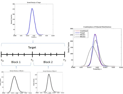
quantities beyond point estimators, such as approximate confidence intervals. Inference is performed by splitting the trading day into blocks where volatility is assumed constant. A
novel combination scheme allows to join the information from all blocks. Both our simulation
study and empirical application demonstrate that the proposed volatility estimator performs
remarkably well even at very high frequencies.
Moreover, we prove a Bernstein - von Mises theorem establishing that, under some
regularity conditions, the generalized fiducial distribution can be approximated by a normal
distribution.
2.2 Introduction
Recently, volatility estimation using high frequency data (HFD) has received considerable
attention in financial econometrics. However, HFD are contaminated by market
process is an It semimartingale is not consistent with observed data. In fact, observed
prices resemble semimartingales recorded with error (MS noise). Consequently, volatility
estimates ignoring microstructure can be heavily biased and, therefore, unreliable for
infer-ence procedures. Moreover, the bias is amplified as the sampling frequency increases, since
market microstructure noise accumulates.
In the standard microstructure setup, the efficient/unobserved log-price process, denoted by Xt=log(St), is assumed to follow an Ito process:
Xt=X0+ ˆ t
0
µsds+
ˆ t
0
σsdWs
where Wt is a standard Wiener process, µt is the drift of the process and σt is the
in-stantaneous variance of the returns. Both µt and σt are adapted locally bounded
ran-dom processes. The process is assumed to evolve in [0, T] and is observed in the grid
Gn={0 =t0 < t1 < ... < tn=T}.The quantity of interest is integrated volatility over the
time period [0, T], namely,
hX, XiT = ˆ T
0
σt2dt
Typically, the observed log-pricesYtm are assumed to be versions ofXtm under the usual
representation
Ytm =Xtm+Utm
where Utm is introduced to capture a variety of effects, including frictions inherent to the
trading process, informational effects and other type of measurement errors, see for example
Aït-Sahalia et al. (2005).
Modeling noise in this simple setup can be unsatisfactory since microstructure frictions
include rounding1. For example, Li and Mykland (2007) analyzed the effect of rounding
on the TSRV estimator and showed that it may not be a robust estimator of integrated
volatility. Rounded Ito processes were initially studied by Jacod (1996) and Delattre and
Jacod (1997) in a non-financial setup. Subsequently, Li and Mykland (2007) and Jacod et al.
(2009) introduced a transition probability so that, conditional onX, observed log-prices Y
1
are distributed aroundX. This new approach allows to endogenize rounding and construct
estimators that are robust in its presence, for example, Jacod et al. (2009). However,
their estimator cannot accommodate the case where the source of error is mainly rounding.
Recently, Li and Mykland (2014) proposed a bias corrected RV estimator when rounding is
the only source of noise. This case is particularly interesting for less expensive stocks, since
rounding is the main source of noise. They showed that the new estimator performs better than the traditional RV estimator as the sampling frequency increases, but cannot reach
very high frequencies such as 1-5 seconds.
In this chapter our goal is to study volatility by taking advantage of the rounding errors.
In particular, we work under the assumption that the latent efficient price process is between
the (rounded) bid-ask prices. Namely, we assume that at any arrival timetm, the process is
contained in the interval[btm, atm], that is
btm ≤Xtm≤atm
where bothbtm andatm are the log versions of the observed bid-ask prices. Volatility
mod-eling in this setup is clearly not affected by rounding and the spread related microstructure
frictions , making the additive component introduced in the aforementioned literature re-dundant. The assumption that the latent efficient price process is between the bid-ask prices
has been used primarily in classical microstructure literature, see Roll (1984), Harris (1990)
and Hasbrouck (1999). However, other intervals that can be justified to contain the latent
price can be a possible candidates. In our empirical study below, besides the direct use of the
spread, we propose a simple way to combine transactions and bid-ask prices to identify such
intervals. Moreover, we work under the additional assumption that volatility is constant ,
that is
Xt=X0+σWt
This approach is similar in spirit with Aït-Sahalia et al. (2005) and Xiu (2010).
In the high frequency volatility literature the parametric approach assumes constant
volatility over a short period of time2. In other words, we split the daily data into blocks
of successive observations and generate samples for each block. Subsequently, we estimate
daily volatility using two methods. The first method computes daily volatility by simply
aggregating the block point estimates and the second method relies on a novel combination
scheme. That is, inference is conducted through a distribution generated by combining
the block distributions into one that summarizes all information from all the blocks under consideration. In a sense, the combination scheme works as an importance sampler by
re-weighing all particles with weights computed through a metric that utilizes the Gaussian
kernel. As we demonstrate, the combined distribution approximates remarkably well the
distribution we would have generated if we had used all data together in one sample.
We test our methodology by conducting a simulation study employing a realistic
simu-lation scheme. We generate our data by simulating the efficient price process in the original
scale and, at observation times, we round the process upwards and downwards, towards the
two nearest ticks. This type of contamination incorporates rounding errors explicitly and
is similar in spirit with the two stage contamination scheme of Li and Mykland (2007) and Jacod et al. (2009). The proposed simulation scheme renders the choice of the starting price
X0relevant, since the magnitude of the spread increases for less expensive stocks, due to the log-transformation, see Li and Mykland (2007, 2014). Therefore, our simulation study uses
different starting prices to capture this effect. For the volatility parameter (signal), in
addi-tion to the standard values in the literature, we use low values since a weak signal introduces
price sluggishness, intensifying the effect of rounding errors. Our simulation study shows
that we can effectively estimate true volatility, constant or stochastic, even in cases where
rounding errors dominate, and outperform the competing parametric and non-parametric estimators.
Finally, our empirical study reveals that robust volatility estimation is possible without
having to assume unrealistic microstructure noise structures. We compare our estimator
2
with the standard parametric and non-parametric alternatives and show that it is very
competitive.
2.3 Generalized Fiducial Inference for HF data
In our setup, we will assume that the efficient log-price follows a Geometric Brownian motion. The process is assumed to evolve in [0, T] and is observed/quoted in the grid
Gn = {0 =t0 < t1 < ... < tn=T}. In addition to the grid Gn, we will consider the
sub-grid Hn = {0 =τ0 < τ1 < ... < τMn =T} ⊆ Gn where volatility is assumed constant for
all ti,m∈(τi−1, τi]. Specifically, in the interval(τi−1, τi]the log-price, given Xτi−1 =xτi−1, evolves according to
dXt=στi−1dWt
In the high frequency literature, it is common practice to to assume thatµ= 0. The order of magnitude of the diffusive component (√dt) is much larger than the order of magnitude
of the drift component (dt), making the drift component mathematically negligible at high
frequencies. Moreover, maintaining it, may have adverse effects on the estimation procedure
since it is estimated with a large standard error. Our preliminary simulation study showed
that maintaining the drift component does not have any impact on the quality of the
gen-erated fiducial distributions. It adds though computational burden and, therefore, it is not included in our reported simulations.
At observation times, within the interval(τi−1, τi], the process is assumed to be between
the bid and ask log-prices
bti,m ≤Xti,m ≤ati,m (2.3.1)
Noting thatWt=
√
tZ whereZ ∼N(0,1)we can re-write equation 2.3.1 as
bti,m ≤στi−1
p
In terms of the fiducial argument, the structural equation is
G(U, ξ) =G(Z, σ) =σ√tZ
The inverse image of G(z, σ)is
Q((b,a],Z) ={σ ∈R+:b< G(z, σ)≤a} (2.3.3)
The corresponding generalized fiducial distribution is
V (Q((b,a], Z))| {Q((b,a], Z)6=∅} (2.3.4)
Generating samples from the generalized fiducial distribution requires the use of Sequential
Monte Carlo (SMC) methods. The SMC algorithm is based on the algorithm developed by
Cisewski and Hannig (2012), where they performed inference for the parameters of normal
linear mixed models and is presented in section 4. In section 5, we prove a Bernstein - von
Mises theorem establishing that, under some regularity conditions, the generalized fiducial
distribution 2.3.4 can be approximated by a normal distribution.
2.4 Estimation Method
2.4.1 Sequential Monte Carlo Algorithm
In this section we present the Sequential Monte Carlo algorithm to generate samples from
the generalized fiducial distribution of the parameters of interest. We consider the interval
(τi−1, τi] where the process is assumed to be between the bid and ask log-prices, as give
by equation 3.3.2. To ease notation we will drop the dependence i and we will embed√t
in Zt such that Zt ∼ N(0, t). We will be denoting Zt1:tm = (Z∆t1, ..., Z∆tm), where ti ∈ {t1, ..., tm},∆ti =ti−ti−1,t0 = 0, and m= 1, ..., n wheren≡ni = #{j, τi−1 < ti,j ≤τi}.
In our setup, Z1,∆tj ∼ N(0,∆tj). The generalized fiducial distribution of the parameters
V Q(bn,an], Zt(1:Kt)n
|nQ(bn,an], Zt(1:Kt)n
6
=∅o (2.4.1)
whereQ(nK) =Q
(bn,an], Zt(1:Kt)n
is the set function containing the values of the parameters
that satisfy the structural equation 3.3.2 for all m ≤ n, given the data (bn,an] and the
generated Zt(1:Kt)n for particle K , where K = 1,2, ..., N. Generating a sample from 2.4.1 is equivalent to simulating sequentially for each m, Zt(1:Kt)m such that Q(mK) is non-empty until
we reach n. The corresponding target distribution up to timetm, denoted byπt1:tm, is
πt1:tm(Zt1:tm |(b,a]t1:tm) ≡ πt1:tm(Zt1:tm) ∝
m Y
j=1 1 (∆tj)
1/2 exp
− 1
2∆tj
Z∆2tj
ICm(Zt1:tm) (2.4.2)
whereICm(Zt1:tm) is an indicator random variable of the set
Cm =
(
Zt1:tm :btj ≤σ
j X
k=1
Z∆tk ≤atj, f or all j= 1, ..., m
)
(2.4.3)
Restriction 2.4.3 is required in order to generate a representative sample from the fiducial
distribution. It ensures that all inequalities up to time tm are satisfied simultaneously. In
practice, this can be achieved easily if at time tm, given that we have sampledZt(1:Kt)m−1, we sampleZ∆(Ktm) by truncating it between the two values
Lm
Zt(1:Kt)m−1
= min
btm−σ
Pm−1
j=1 Z (K) 1,∆tj
σ , σ∈Q
(K)
m−1
Rm
Zt(1:Kt)m−1= max
atm−σ
Pm−1
j=1 Z (K) 1,∆tj
σ , σ∈Q
(K)
m−1
Utilizing these type of restrictions we can write
ICm(Zt1:tm) = ICm−1(Zt1:tm)I(Lm,Rm)(Z1,∆tm) =
m Y
j=1
I(Lj,Rj) Z1,∆tj
The proposal distribution for our SMC algorithm utilizes the Cauchy distribution
˜
πt1:tm(Zt1:tm|(b,a]t1:tm)≡π˜t1:tm(Zt1:tm) ∝πt1(Zt1)
m Y
j=2
1 (∆tj)
1/2
1 + Z 2
tj
∆tj
(F(Rj)−F(Lj))
I(Lj,Rj) Z∆tj
(2.4.4)
where F denotes the cdf of the Cauchy distribution. It is important to point out that
the proposal distribution treats Zt1 as unrestricted, that is, Zt1 is drawn from the target
distribution. The reason is that Zt1 will be used to identifyQ (K) 1 =Q
(bt1, at1], Z (K)
t1
, for
each particleK , whereK= 1,2, ..., N. This generates the interval
bt1
Z1,∆t1
, at1
Z1,∆t1
and, clearly, any σ in this interval satisfies the first set of inequalities. The rest of the
inequalities will be used sequentially to trim the interval in a way that all inequalities will be satisfied.
The conditional proposal distribution for m >1, which will be used to draw samples in the algorithm is
e
πtm|t1:tm−1 ∝
I(Lm,Rm)(Z1,∆tm)
(∆tm)
1/2 1 + Z
2
tm
∆tm
(F(Rm)−F(Lm))
(2.4.5)
The final component of the algorithm is the importance weights. The weights are computed
as
Wt1:tm = πt1:tm
˜
πt1:tm
= πtm|t1:tm−1πt1:tm−1 ˜
πtm|t1:tm−1π˜t1:tm−1
=WtmWt1:tm−1 (2.4.6)
where
Wtm =
πtm|t1:tm−1 ˜
is the incremental weight. The incremental weight is given by
Wtm ∝exp
− 1
2∆tm
Zt2m 1 + Z 2
tm
∆tm
(F(Rm)−F(Lm)) (2.4.7)
2.4.2 Resampling - Alteration Step
In our setup the resampling step resembles that of a general SMC algorithm. To overcome the degeneracy of the particle system as tm increases, we measure the effective sample size
(ESS) at timetm
ESStm =
PN k=1W
(k)
t1:tm 2
/PN k=1
Wt(k)
1:tm 2
(2.4.8)
and if the ESS for the particle system has dropped below a designated threshold (usually N/2), the particle system is resampled removing the particles with low weights and replicating the particles with higher weights. In this setup, replicating particles will not generate a
representative sample of the fiducial distribution. As mentioned above, each of the particles
forms an interval in the parameter space, and therefore, if the particles are simply copied,
the intervals will be concentrated in a narrow area, due to particles with initially higher
weight. Moreover, as the algorithm progresses, the particles will not be able to move from
those regions. A solution to this issue is to alter the particles selected from resampling in
a way that they will maintain their heavy weight, while still allowing for an appropriate
sample of the fiducial distribution.
The alteration step is performed as follows: Suppose that at timetmparticleKis selected
in the resampling step and will be copied. Up to time tm, we have observed the following
inequalities (We are suppressing the dependence inK):
bm≤σVmZm≤am
We perform the following decomposition forZm
Zm=kZmk
Zm
kZmk
The SMC algorithm
Step Action
1. Initialization Fork= 1,2, ..., KdrawZt(1k)∼πt1 (Eq. 2.4.2) and setW (k)
t1 = 1 2. Fortm> t1andtm≤tn Fork= 1,2, ..., KdrawZt(mk)∼eπtm|t1:tm−1 (Eq. 2.4.5)
3. Fortm> t1andtm≤tn Calculate weightsW
(k)
t1:tm=W
(k)
tmW
(k)
t1:tm−1 (Eq. 2.4.6)
4. Fortm> t1andtm≤tn CalculateESStm (Eq. 2.4.8). IfESStm ≤thresholdgo to step 5.
Else go to step 2 and setm=m+ 1
5. FortmgivenESStm≤thd Resample particles and setWt1:tm =N
−1
. Go to step 6.
6. Fortm Perform alteration as described above and setm=m+ 1
where kZmk denotes L2 norm of Zm. By setting D=kZmk and κ = kZZmmk decomposition
2.4.9 can be re-written as
Zm =Dκ (2.4.10)
Moreover, by assumption Zm ∼N(0,Im), therefore, D∼ p
χ2
m .
Decomposition 2.4.9 allows us to alterZm by sampling new values ofDaccording to its
distribution. If we denote by De the generated values, then we can useZem =Dκe to update
the set
Qm ={σ :bm ≤σVmZm≤am}
We achieve that by noting that, sinceσsolvesbm ≤σVmZm ≤am, then we need to identify
e
σ that solvebm≤eσVmZem≤am. Using the following equality
σVZm =σVDκ=eσVmDκe =eσVmZem
we can solve for eσ, that is
e
σ =σD
e
D
The table below gives an outline of the steps of the algorithm.
2.5 Theoretical Results
2.5.1 Preliminaries - Likelihood of Exact Data
Furthermore, assume that ti−ti−1 = ∆, fixed. Specifically, the log-price, given Xt0 =x0, evolves according to
Xt=x0+σWt
Suppose we fully observe the process. Then, the corresponding likelihood is
L σ2,Xn
=
n Y
i=1
p Xti |Xti−1
where, p Xti |Xti−1
= 2πσ2∆−1/2expn− 1
2σ2∆ Xti−Xti−1
2o
. The log-likelihood is
l σ2,Xn
=−n
2 log 2πσ 2∆
− 1
2σ2∆
n X
i=1
Xti−Xti−1
2
The score is
˙
l σ2,Xn
=− n
2σ2 + 1 2σ4∆
n X
i=1
Xti−Xti−1
2
=− n
2σ2 +
n
2σ4σˆ 2
n
where σˆ2n = n1∆Pni=1 Xti−Xti−1
2
is the MLE, i.e., the solution to the score equation.
Taking the expectation under the true parameterσ02 we have thatEl σ˙ 2,Xn
= 0. The derivation of the Fisher information relies on
¨
l σ2,Xn
= n
2σ4 − 1
σ6∆
n X
i=1
Xti−Xti−1
2
= n 2σ4 −
n σ6σˆ
2
n
Denote byIn the Fisher Information, derived from
In=E−¨l σ2,Xn
= n
2σ40 =nI0
whereI0 = 2σ14 0
2.5.2 Likelihood of Rounded Data
The data are observed with rounding errors which occur in the original scale. Therefore, if
αn denotes the accuracy of the measurement, then, by denotings(αn) =αnbs/αnc, we have
that at arrival times Gn={0 =t0 < t1< ... < tn=T}
S(αn)
ti ≤Sti ≤S
(αn)
ti +αn
Therefore, we observe Rn = [bt1, at1]× · · · ×[btn, atn], such that bti = logS
(αn)
ti and ati =
logS(αn)
ti +αn
. This implies
bti ≤Xti ≤ati
LetX? be an independent copy ofX such thatbti ≤X
?
ti ≤ati. To state this differently,
X? ∼ 1RnL Xn, σ
2
L(σ2, R
n)
We are interested in the probability/likelihood of the dataRn.
L σ2, Rn
= ˆ at1
bt1
p Xt?1 |xt0
dXt?1· · ·
ˆ atn
btn
pXt?n |Xt?n−1dXt?n = ˆ
Rn
L σ2,X?n
dX?n (2.5.1)
Lemma 1. Denote byl σ2, Rn
= logL σ2, Rn
the log-likelihood 2.5.1. The score equation
is given by
˙
l σ2, Rn
= n
2σ4 E σˆ 2?
n |X?n∈Rn
−σ2
The solution to the score equation yields a “maximum likelihood estimator”. That is
σR2n =E σˆn2? |X?n∈Rn
where σˆn2? = n1∆Pni=1
Xt?i−Xt?i−1
2
is the MLE had we observed the the data Xn. The
expectation is taken with respect to the density 1RnL(Xn,σ
2)
L(σ2,R
n) . The Fisher information is E−¨l σ2, Rn
=In− I2
where V ar σˆ2?
n |X?n∈Rn
= E σˆ2? n −σ2Rn
2
|X? n∈Rn
and the expectation is taken
under the true value σ02.
Remark 1. The second term on the RHS of the Fisher Information expresses the loss of
information due to the discretization error.
Denote the local parameter by h =√n σ2−σ02
and the corresponding log-likelihood
by lRn,h =l σ
2 0+h/
√
n, Rn. Expanding the log-likelihood around the local parameter we
have that
lRn,h−lRn,0= h √
nl σ˙
2 0, Rn
+ 1 2
h2 n¨l σ
2 0, Rn
+Remn,h (2.5.2)
whereRemn,h= 16 h
3
n3/2 ...
lRn σ¯
2, R
n
for some σ¯2 such that σ2
0 ≤σ¯2 ≤σ20+h/n. Recall that
In= 2nσ4 0
, then we can easily show that
˙
l σ02, Rn
=In E σˆn2? |X?n∈Rn
−σ20 (2.5.3)
and
¨
lRn σ
2 0, Rn
=−In 1− InV ar σˆn2? |X?n∈Rn
− 2
σ2 0
In E σˆn2? |X?n∈Rn
−σ02
(2.5.4)
Substituting equations 2.5.3 and 2.5.4 in equation 2.5.2 we have that
lRn,h−lRn,0 = h √
nIn E σˆ
2?
n |X?n∈Rn
−σ02− h
2
2nIn 1− InV ar σˆ
2?
n |X?n∈Rn
− h
2
nσ02In E σˆ
2?
n |X?n∈Rn
−σ02
+Remn,h
= √h
nIn E σˆ
2?
n |X?n∈Rn
−σ02
− h
2
2nIn 1− InV ar σˆ
2?
n |X?n∈Rn
+Remn,h+op(1)
(2.5.5)
Theop(1)term in equation 2.5.5 stems from the fact that once we establish the behavior of
the score function, that is, √1
nl σ˙
2 0, Rn
, then
1
nσ02In E ˆσ
2?
n |X?n∈Rn
−σ02
= √1 nσ20
1
√ n
˙
l σ20, Rn
Denote
Sn=
1
√
nIn E σˆ
2?
n |X?n∈Rn
−σ02
and
Fn=
1
nIn 1− InV ar σˆ
2?
n |X?n∈Rn
Then, equation 2.5.5 becomes
lRn,h−lRn,0 =Snh−
1 2Fnh
2+Rem+o
p(1) (2.5.6)
2.5.3 Approximation of the distribution of the score equation
To simplify the notation, we fix T = 1 and ti − ti−1 = ∆ = n1 or simply ti = ni.
Before we prove the theorem, we need to understand the behavior of the quantity
√
n E σˆn2? |X?n∈Rn
−σˆn2?
, since we can rewrite the score equation as
1
√
nIn E σˆ
2?
n |X?n∈Rn
−σ02= √1
nIn E σˆ
2?
n |X?n∈Rn
−σˆ2n?+√1 nIn σˆ
2? n −σ20
Consider the collection of σv-fields Fk,n =σ{X1?, . . . Xk?, Rn} for k ≤ n. Clearly, Fk−1,n ⊆
Fk,n. Then, denote
ξn,k=E σˆn2? | Fk−1,n
−E σˆ2n?| Fk,n
which is a martingale difference. Notice that
E σˆn2 | F0,n
−σˆn2 =
n X
k=1
ξn,k
which is a martingale. Then, there is a constantC such that
|ξn,k| ≤Cα2n
The following lemma states Azuma’s inequality without proof.