THE TAXONOMIC AND FUNCTIONAL NATURE OF PLANT-ASSOCIATED MICROBIOMES
Scott MacKay Yourstone
A dissertation submitted to the faculty at the University of North Carolina at Chapel Hill in partial fulfillment of the requirements for the degree of Doctor of Philosophy in the Curriculum of Bioinformatics and Computational Biology.
Chapel Hill 2017
Approved by: Jeffery Dangl Corbin Jones Piotr Mieczkowski
ii ©2017
iii ABSTRACT
Scott MacKay Yourstone: The Taxonomic and Functional Nature of Plant-Associated Microbiomes
(Under the direction of Jeffery Dangl and Corbin Jones)
Microbes live in close association with eukaryotes and have substantial impacts on fitness and well-being of their hosts. In plants, microbes can colonize soil adjacent to plant roots and can even survive inside of plant tissues. They can have either positive or negative effects on plant fitness and therefore show potential for use as an agricultural tool. However, our current understanding of how these microbial communities are formed and how they function is limited.
iv
plants. Communities associated with different Arabidopsis ecotypes and ages have only minor differences.
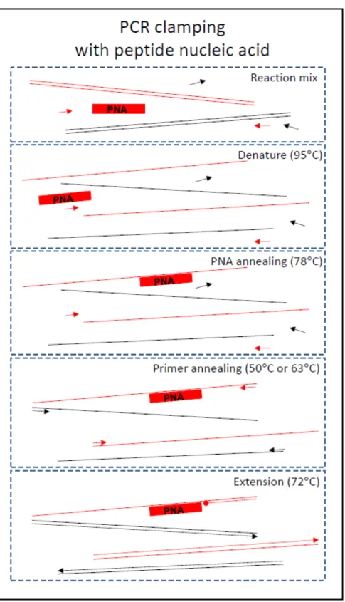
Chapter 3 presents improved methods for profiling taxa in plant-associated microbiomes by utilizing two techniques. First, PCR amplification clamps designed from peptide nucleic acids are used to reduce plant chloroplast contamination. Removing unwanted chloroplast contamination reduces the cost of sequencing by increasing the yield of usable, bacterial 16S reads. Second, 16S amplicons are tagged with a unique DNA oligo (i.e. molecule tag) prior to PCR amplification. After PCR amplification and sequencing, reads having the same molecule tag likely originated from the same DNA template. Therefore, discrepancies between these reads are presumably sequencing errors and can be corrected bioinformatically. Identifying and correcting these sequencing errors can be performed using the MTToolbox software described in Chapter 4. Correcting sequencing errors using molecule tagged reads and MTToolbox substantially reduces the number of spurious singleton OTUs.
v
rhizosphere colonization. Therefore, identifying taxa specific enrichments patterns is important for understanding mechanisms associated with rhizosphere colonization.
vi
vii
ACKNOWLEDGEMENTS
This work represents collaborative efforts from a large number of people. First I would like to acknowledge and thank my major professors—Jeff Dangl and Corbin Jones. Working with them has been a pleasure. They have provided countless hours of help and tutelage that has contributed to my growth as a scientist. Without their efforts this would have been impossible.
One of the best things about working in the Dangl lab is the great people that I get to associate with on a daily basis. The Dangl lab members are all accomplished scientists. Their advice and assistance has been invaluable. I have thoroughly enjoined the numerous scientific discussions I have had with each of them. Many current and former lab members have contributed useful suggestions, advice, and efforts to this work. I respect and admire their work ethic and commitment to exceptional science. Beyond having a fantastic working relationship with members of the Dangl lab, I consider them some of my best friends.
I am also grateful for my committee members—Jeff Dangl, Corbin Jones, Jan Prins, Piotr Mieczkowski, and Fernando Pardo-Manuel de Villena. I have had the privilege of working with each of them individually and greatly appreciate the time and energy they have committed on my behalf.
viii
Lastly, I would like to thank my family for their support and encouragement over the last seven years—especially my parents and my wife, Erin. They have provided unwavering support in all aspects of my life, and have helped me become the best version of myself.
ix
TABLE OF CONTENTS
LIST OF ABBREVIATIONS ... xiii
LIST OF FIGURES ... xiv
CHAPTER 1: INTRODUCTION ...1
2.1 Impact and Significance of microorganisms ... 1
2.2 Observing the microbiome using the 16S ribosomal gene ... 2
2.3 Observing the microbiome using shotgun sequencing ... 6
CHAPTER 2: DEFINING THE CORE ARABIDOPSIS THALIANA ROOT MICROBIOME ...12
2.1 Overview ... 12
2.2 Introduction ... 13
2.3 Results ... 14
2.4 Methods ... 27
2.4.1 General strategy ... 27
2.4.2 Soil collection and analysis ... 28
2.4.3 Seed sterilization and germination ... 28
2.4.4 Seedling growth ... 29
2.4.5 Harvesting ... 30
2.4.6 DNA extraction ... 32
2.4.7 PCR ... 33
2.4.8 454 pyrotag sequencing ... 33
2.4.9 Primer test and technical reproducibility ... 34
2.4.10 Primer specificity sequence ... 35
2.4.11 Sequence processing pipeline and assignment of OTUs ... 35
2.4.12 Detection of differentially enriched OTUs by the GLMM ... 38
2.4.13 Partial GLMM ... 39
x
2.4.15 Heat maps ... 40
2.4.16 Diversity ... 40
2.4.17 Rarefaction curves ... 41
2.4.18 Taxonomy histograms and statistics ... 41
2.4.19 Sample clustering using UniFrac ... 41
2.4.20 CARD–FISH application to roots ... 42
2.4.21 Sample naming in OTU tables ... 44
2.5 Supplemental Figures ... 45
CHAPTER 3: PRACTICAL INOVATIONS FOR HIGH-THROUGHPUT AMPLICON SEQUENCING ...64
3.1 Overview ... 64
3.2 Introduction ... 64
3.3 Results ... 65
3.4 Methods ... 75
3.4.1 Cloned 16S template ... 75
3.4.2 Root EC, soil and leaf DNA extraction and quantification ... 75
3.4.3 Peptide nucleic acid (PNA) design ... 76
3.4.4 Primer design ... 77
3.4.5 Template tagging with molecular tagging–frameshifting primers ... 78
3.4.6 PCR using tagged templates (our method) ... 80
3.4.7 PCR using untagged templates (EMP method) ... 81
3.4.8 Quantification of PCR products and library mixing ... 81
3.4.9 Library denaturation, dilution and sequencing ... 82
3.4.10 Demultiplexing ... 84
3.4.11 Raw sequence processing (our method) ... 84
3.4.12 Raw sequence processing (EMP method) ... 86
3.4.13 Operational taxonomic unit (OTU) formation ... 86
3.4.14 OTU table construction ... 87
3.4.15 Assigning taxonomy to OTUs ... 87
3.4.16 Predicting pPNA and mPNA utility across diverse plant families ... 88
3.4.17 Subsampling ... 88
3.4.18 Permutation tests ... 88
xi
3.4.20 Chi-squared tests ... 89
3.5 Supplemental Figures ... 90
CHAPTER 4: MT-TOOLBOX: IMPROVED AMPLICON SEQUENCING USING MOLECULE TAGS ...112
4.1 Overview ... 112
4.2 Background ... 113
4.3 Implementation ... 115
4.4 Results ... 119
4.5 Conclusions ... 123
4.6 Supplemental Information ... 123
4.6.1 Building the Alignment Matrix ... 123
4.6.2 Single Read Categories ... 123
4.6.3 Optimizing ConSeqs Accuracy ... 124
4.6.4 Filtering ‘birthday paradox’ ConSeqs Using the c-score ... 125
4.6.5 MT-MT-Toolbox (MeTagenomics Edition) ... 126
4.6.6. BioUtils ... 126
4.6.7 Digital Normalization ... 127
4.6.8 Cluster Parallelization ... 127
4.6.9 Clonal Plasmid Accuracy ... 128
4.6.10 Protocols Compatible with MT-Toolbox ... 128
4.7 Supplemental Figures ... 129
CHAPTER 5: RHIZOSPHERE ENRICHED FUNCTIONS IN ARABIDOPSIS THALIANA MICROBIAL COMMUNITIES ...141
5.1 Overview ... 141
5.2 Introduction ... 142
5.3 Results ... 146
5.3.1 DAFE Uses Metagenomic Sequence Data More Efficiently Than Common Approaches ... 146
5.3.2 DAFE Identifies Rhizosphere Enriched Functions ... 149
5.3.3 Impact of Host Age on the Rhizosphere Community ... 160
5.3.4 Genotype Effects on Rhizosphere Colonization and Function ... 163
5.3.5 Rare Genes Appear to be Critical for Rhizosphere Enrichment ... 164
xii
5.5 Biological Insights ... 167
5.6 Conclusions ... 169
5.7 Methods ... 170
5.7.1 DAFE Algorithm ... 170
5.7.2 Reference Genome Database ... 171
5.7.3 Metagenome Assembly ... 172
5.7.4 Samples and Sequencing ... 172
5.7.5 En Masse Culturing and Sequencing ... 172
5.7.6 Defining OrthoGroups ... 174
5.7.7 Tree Generation ... 174
5.7.8 Rare Gene Analysis ... 175
5.8 Supplemental Figures ... 176
xiii
LIST OF ABBREVIATIONS
DAFE Differentially Abundant Functional Elements
xiv
LIST OF FIGURES
Figure 2.1 Sample fraction and soil type drive the microbial composition of root
associated communities ...33
Figure 2.2 Taxonomic distributions of measurable OTUs ...36
Figure 2.3 Dot plots of notable OTUs ...39
Figure 2.4 CARD-FISH confirmation of Actinobacteria on roots ...41
Figure. 2.5 Harvesting scheme ...62
Figure 2.6 Primer test and technical reproducibility ...63
Figure 2.7 Informatics pipeline ...64
Figure 2.8 Sequencing statistics and quality ... 65
Figure 2.9 Sample fraction and soil type drive the microbial composition of root-associated endophyte communities ... 66
Figure 2.10 OTUs from four biological replicates are reproducible ... 67
Figure 2.11 OTUs that differentiate endophyte compartment and rhizosphere from soil ... 69
Figure 2.12 Overlap of GLMM predictions ... 71
Figure 2.13 Taxonomic classifications at the family level are robust to method ... 72
Figure 2.14 Test for PCR bias in pyrotagging ... 73
Figure 2.15 Dot plots of notable OTUs ... 75
Figure 2.16 Quantification using CARD-FISH ... 76
Figure 2.17 Sequencing of sterile seedlings ... 77
Figure 2.18 Genotype variability colored by sequencing plate ... 79
Figure 2.19 Phyla in each fraction by soil type ... 80
Figure 3.1 Molecular tagging reduces sequencing error for a clonal template ... 83
Figure 3.2 Molecular tagging lowers estimates of alpha diversity and improves technical reproducibility ... 86
xv
Figure 3.4 Reference map of the 16S rRNA gene ... 108
Figure 3.5 Schematic of molecular taggin ... 109
Figure 3.6 Frameshifting primers enhance library diversity ... 110
Figure 3.7 MiSeq run quality for Run A and Run B ... 111
Figure 3.8 MiSeq run quality for Run C and Run D ... 112
Figure 3.9 Template tagging, PCR, sequencing, and molecular tag processing workflow ... 114
Figure 3.10 An MT of 13 random bases is sufficiently unique ... 115
Figure 3.11 Beta diversity conclusions ... 117
Figure 3.12 PNA schema ... 119
Figure 3.13 Exhaustive search for PNA oligonucleotide candidates ...120
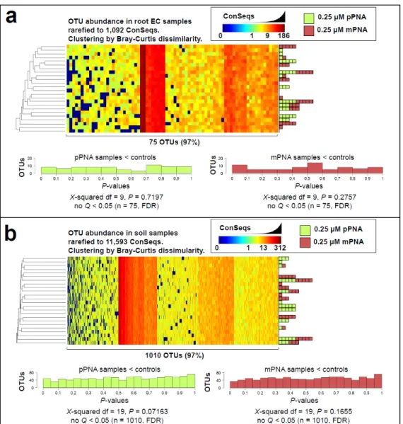
Figure 3.14 No bacterial OTUs are affected by pPNA or mPNA ... 121
Figure 3.15 No bacterial family abundances are affected by pPNA or mPNA ... 122
Figure 3.16 Diverse plant species for which PNA should block ... 123
Figure 3.17 Predicted specificity of PNAs using Sakai et al ... 125
Figure 3.18 Template tagging primer variants were evenly mixed and properly recovered ... 126
Figure 3.19 Universal PCR primers can be used to amplify and barcode other tagged templates ... 128
Figure 3.20 Primer linkers ... 129
Figure 4.1 MT-Toolbox overview ... 134
Figure 4.2 Read and MT counts per sample ... 138
Figure 4.3 MT depth histograms for each sample ... 139
Figure 4.4 ConSeqs error profile ... 140
Figure 4.5 Implementation of molecular tags used in Lundberg et al ... 147
xvi
Figure 4.7 Length distribution of reads is narrow ... 149
Figure 4.8 The number and types of errors seen in ConSeqs ... 150
Figure 4.9 Accuracy of ConSeqs ... 151
Figure 4.10 Schematic of overlapping PE-reads ... 152
Figure 4.11 C-score distributions for ConSeqs ... 153
Figure 4.12 Correlation between c-score and errors ... 154
Figure 4.13 Screen shot of MT-Toolbox GUI ... 155
Figure 4.14 BioUtils is faster than BioPerl ... 156
Figure 4.15 ConSeq error profile ... 157
Figure 4.16 Analysis of higher error per base in sample 100x B ... 158
Figure 5.1 Genome database and metagenome summary ... 166
Figure 5.2 Enrichments between rhizosphere and bulk soil using COG Categories ... 169
Figure 5.3 Five most frequently enriched COGs ... 171
Figure 5.4 Limitations of COGs in metagenome analyses ... 173
Figure 5.5 Example OGs with rhizosphere and bulk soil enriched functions ... 176
Figure 5.6 Age effects ... 180
Figure 5.7 Rhizosphere-enriched gene are more frequently rare genes ... 183
Figure 5.8 DAFE algorithm ... 192
Figure 5.9 Read per metagenome sample ... 193
Figure 5.10 Bases per metagenome sample ... 193
Figure 5.11 Example pictures of en masse culturing ... 194
Figure 5.12 Conservation score example ... 195
Figure 5.13 Reads mapped to genomes from different environments ... 196
xvii
Figure 5.15 Differentially abundant COGs at 60% identity mapping ... 198
Figure 5.16 Pfam and KO annotations per genome ... 199
Figure 5.17 Old soil vs yng soil COG categories ... 200
Figure 5.18 Bradyrhizobium species tree ... 201
Figure 5.19 Plant Genotype enrichments ... 202
1
CHAPTER 1: INTRODUCTION
2.1 Impact and Significance of microorganisms
Microorganisms colonize nearly every inhabitable environment and constitute the majority of biodiversity on the earth. The impacts of microorganisms are substantial; understanding the characteristics of these microbes and the communities in which they associate (i.e. microbiota) is thus of great importance.
2
Microbes can also protect plants against pathogens. For example, some microbes such as Pseudomonas simiae WCS417 can prime the plant immune system causing induced systemic resistance (ISR) (Berendsen et al. 2015; Stringlis et al. 2017). During ISR the plant immune system is stimulated, providing increased resistance to pathogens without fully engaging the immune system. Because a fully engaged immune system requires a substantial amount of resources, the plant can divert those resource to other needs and still remain resistant to pathogens increasing overall fitness (Vos, Pieterse, and Van Wees n.d.).
Because microbes can have an enormous impact on plant fitness, understanding how plants shape and interact with their associated microbes is vital. Furthermore, as we seek to feed a growing global population with limited resources, utilizing the power of microbes as an agricultural tool has enormous potential.
2.2 Observing the microbiome using the 16S ribosomal gene
Observing microbes in their natural environments (i.e. microbiome) has been a challenge. Microbiomes may contain millions of members drawn from a diverse part of the tree of life. A few individual community members may be cultured in artificial conditions, but these culture-based methods can only capture a fraction of a microbiota. Furthermore, observations made using culture-based methods may not accurately reflect the state of wild microbiomes because they have been removed from their natural habitat. New and rapid developments in DNA sequencing technology and computational resources have provided unique opportunities to explore these communities in their natural settings. Therefore, our knowledge and interest in microbiomes is increasing as these novel tools are invented and expanded
3
genes were selected for measuring microbial communities for three main reasons. First, for eubacteria, the 16S gene encodes a crucial component of the ribosome, a complex structure required for the basic and universal process of translating messenger RNA into proteins, this ribosomal gene is highly conserved across the tree of life (Woese, Fox, and Zablen 1975; Woese and Fox 1977). Consequently, it can be used to detect all bacteria present in a microbiome. Second, despite being highly conserved, some regions of this gene are extremely variable. These variable regions provide the phylogenetic resolution required to differentiate between species. And third, the variable regions in the gene are flanked by highly conserved regions that make excellent targets for designing PCR primers to amplify the variable regions. Therefore, a single primer pair matching conserved regions in the gene can provide taxa specific sequences representing the diversity of microbes contained in a microbiome.
4
to efficiently cluster sequence reads into OTUs. First, identical reads are identified and collapsed into a single read. Reads that are represented multiple times likely originate from the most abundant microbes and are unlikely to contain sequencing errors. Consequently, in the subsequent clustering step they are used as starting points from which clusters can expand. Compared against previous OTU building algorithms, this heuristic algorithm decreases run time without substantially reducing accuracy of clusters (Edgar 2010).
The resulting list of OTUs and their abundance, as measured by the number of reads contained in the OTU cluster, constitutes a 16S profile of a microbiome. A profile from a single microbiome can be described by its species diversity (alpha diversity; Whittaker 1972). Furthermore, profiles from different microbiomes can be compared (beta diversity) using distance/similarity metrics like Bray-Curtis and Unifrac (C. Lozupone and Knight 2005a; Bray and Curtis 1957). Various ordination methods such as principal coordinate analysis (PCoA) are a useful tool to visualize the pairwise similarities and differences between 16S profiles of microbiomes. Individual OTUs or their taxonomic groupings can be tested for differential abundance across microbiomes using linear models. Representative sequences from each OTU can be compared against extensive 16S gene databases such as greengenes and SILVA (DeSantis et al. 2006; Yilmaz et al. 2014; Quast et al. 2012) to describe the taxonomic attributes of a microbiome.
5
culturing. Lastly, 16S sequencing can capture a large fraction of the community even down to members that are rare. As sequencing throughput continues to increase, the ability to capture rare microbes will only increase.
These 16S-based methods have been successfully used to describe multiple plant-associated microbiomes. These studies have investigated which microbial taxa colonize a given environment and how those taxonomic profiles change across fractions, soils, plant physiology and environmental conditions. The taxa inhabiting the endosphere (inner parts of the roots) are different from those found in the rhizosphere or bulk soil (Lundberg et al. 2012; Bulgarelli et al. 2012a). Furthermore, there are few taxa that differ between two developmental stages of adult plants and across multiple Arabidopsis ecotypes suggesting that some genotypic differences are not strongly associated with the assembly of the microbiome. However, in other plant species, such as potatoes, genotypic differences have a larger impact on the structure of the microbiome (Bulgarelli et al. 2013; Knief et al. 2010; Wagner et al. 2016). Additionally, common garden experiments demonstrated clear differences between the rhizosphere and endosphere microbiomes across plant species indicating that plants actively select their microbiome (Ofek et al. 2014). However, within more closely related plant species such as those in the Brassicaceae family, the differences between rhizosphere microbiota cannot be explained by host phylogenetic distance alone (Schlaeppi et al. 2014).
6
DNA extraction biases can preferentially amplify the 16S gene for certain taxa and some taxa have multiple 16S gene copies making it difficult to accurately measure the abundance of these taxa (Hong et al. 2009; Sharpton et al. 2011; Logares et al. 2014; Větrovský and Baldrian 2013). Fourth, 16S profiling is primarily focused on describing the taxa that inhabit a microbiome and is limited to the extent to which it can describe the functional attributes. Tools like PICRUSt and Tax4Fun map 16S reads to a reference database of genomes that are then used to infer the metagenome (Langille et al. 2013; Aßhauer et al. 2015). However, such tools are limited by the resolution of an OTU cluster. This dilemma is demonstrated by the observation that bacteria with identical 16S sequences can harbor different functional repertoires—for example, within Escherichia coli alone genome size and content can vary considerably (Lukjancenko, Wassenaar, and Ussery 2010; Bergthorsson and Ochman 1995). Additionally, inference of metagenomes from 16S profiles is also limited by how accurately the database reflects that taxa present in the microbiome. But because isolate genomes are being sequenced at an inspiring rate, this problem is diminishing.
2.3 Observing the microbiome using shotgun sequencing
7
A variety of methods exist for analyzing metagenomic sequences. The majority of such methods rely on either de novo assembly of the reads or mapping reads to a reference database or a mixture of both (Oulas et al. 2015). De novo assembly of a metagenome attempts to reconstruct each genomic sequence from a set of short DNA sequences (i.e. reads). These short reads can be assembled into longer sequence fragments (i.e. contigs and scaffolds) using standard genome assembly algorithms (A Bankevich 2012; Zerbino and Birney 2008) or specialized algorithms designed specifically for assembling metagenomes (Namiki et al. 2012; Boisvert et al. 2012; Vollmers, Wiegand, and Kaster 2017; Peng et al. 2012, 2011). De novo assembly of metagenomes has successfully been applied to the reconstruction of complete genomes of microbes present in simple communities (Albertsen et al. 2013).
8
encounters a region with low coverage it breaks. Therefore, assemblies of low coverage genomes frequently contain many short contigs. To fully assemble low abundance community members, a substantial amount of sequencing is required. However, sequencing more reads can be wasteful because the majority of the new sequences are from the high abundance genomes that have already been assembled. Therefore, the species unevenness of microbiota are a substantial impediment to de novo assembly. Computational methods for evening out the abundance differences have improved de novo assembly of complex microbiota (Howe et al. 2014; Crusoe et al. 2015). However, such computational solutions will never resolve the overabundance of sequences wasted on high-abundance microbes.
9
The second primary method for analyzing metagenome reads involves mapping reads to a database of reference sequences. These databases can be compiled from individual genomes of previously sequenced isolates, annotation databases (e.g. COG, KEGG, SEED), gene catalogs, or contigs assembled from metagenomes. Reads can be mapped using standard read mapping software (H. Li and Durbin 2009, 2010; Miyazawa 1995). The number of reads mapping to each genomic feature is an estimation of the abundance of that feature in the microbiome. These feature abundances can be compared across metagenomes using software such as STAMP and MG-RAST (Parks et al. 2014; Keegan, Glass, and Meyer 2016) to infer functions potentially important for survival and colonization of a microbiome. The primary limitation to mapping metagenome reads to a reference database is the bias imposed by the database. Features in the metagenome that are not represented in the database will not be measured.
10
rhizosphere, particularly those encoding for microbe-plant and microbe-microbe interactions, were under positive selection (Bulgarelli et al. 2015).
Despite the recent progress in understanding the functional profiles of microbiomes, there are still substantial knowledge gaps. First, most comparative metagenomics studies only describe functional differences between microbiomes at a general level (Bulgarelli et al. 2015). Higher resolution comparisons to identify specific functions in specific taxa are important for generating actionable knowledge. As these specific traits are identified they can be experimentally validated and explored. Second, metagenome studies primarily focused on patterns of colonization. Experiments that identify functional mechanisms involved in growth promotion and other important traits should also be a point of focus. Third, observing plant endophytic metagenomes is nearly impossible because nearly all shotgun sequences from these samples are predominantly host plant DNA. Methods for separating bacterial and plant DNA prior to or during sequencing would be invaluable. Lastly, metagenomics has been useful in describing the functional potential of microbiomes, but it remains unclear how microbes modulate their gene expression across different environments. Therefore, coupling metagenomics and metatranscriptomics is important for accurately and completely describing the functional characteristics of microbiomes.
11
12
CHAPTER 2: DEFINING THE CORE ARABIDOPSIS THALIANA ROOT
MICROBIOME1
2.1 Overview
Land plants associate with a root microbiota distinct from the complex microbial community present in surrounding soil. The microbiota colonizing the rhizosphere (immediately surrounding the root) and the endophytic compartment (within the root) contribute to plant growth, productivity, carbon sequestration and phytoremediation (Rodriguez et al. 2008; De Deyn, Cornelissen, and Bardgett 2008; van der Lelie et al. 2009). Colonization of the root occurs despite a sophisticated plant immune system (Jones and Dangl 2006; Dodds and Rathjen 2010) suggesting finely tuned discrimination of mutualists and commensals from pathogens. Genetic principles governing the derivation of host-specific endophyte communities from soil communities are poorly understood. Here we report the pyrosequencing of the bacterial 16S ribosomal RNA gene of more than 600 Arabidopsis thaliana plants to test the hypotheses that the root rhizosphere and endophytic compartment microbiota of plants grown under controlled conditions in natural soils are sufficiently dependent on the host to remain consistent across different soil types and developmental stages, and sufficiently dependent on host genotype to vary between inbred Arabidopsis accessions. We describe different bacterial communities in two
1 The content of this chapter has been published before as a peer-reviewed article (Lundberg et al., 2012). Figures
13
geochemically distinct bulk soils and in rhizosphere and endophytic compartments prepared from roots grown in these soils. The communities in each compartment are strongly influenced by soil type. Endophytic compartments from both soils feature overlapping, low-complexity communities that are markedly enriched in Actinobacteria and specific families from other phyla, notably Proteobacteria. Some bacteria vary quantitatively between plants of different developmental stage and genotype. Our rigorous definition of an endophytic compartment microbiome should facilitate controlled dissection of plant– microbe interactions derived from complex soil communities.
2.2 Introduction
14
Microbial community structure differs across plant species (Redford et al. 2010; Hardoim, van Overbeek, and Elsas 2008), and there are reports of host-genotype-dependent differences in patterns of microbial associations (Inceoğlu et al. 2010; İnceoğlu et al. 2011). However, the divergent methods used in those studies relied on small sample sizes and low-resolution phylotyping techniques potentially confounded by off-target sequences and chimaeric amplicons. We developed a robust experimental system to sample repeatedly the root microbiome using high-throughput sequencing. Our results confirm many of the general conclusions from earlier studies and, because of controlled experimental design and the power of deep sequencing, provide a key step towards the definition of this microbiome’s functional capacity and the host genes that potentially contribute to microbial association phenotypes. Such plant genes would constitute major agronomic targets.
2.3 Results
15
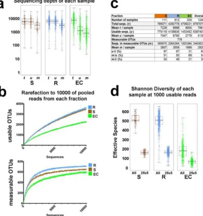
units (OTUs), reduced noise and removed chimaeras. We determined technical reproducibility thresholds to conclude that OTUs defined by ≥ 25 reads in ≥ 5 samples (hereafter 253 5) are individually ‘measurable OTUs’ (Benson et al. 2010; Gottel et al. 2011) (Figures 2.6 and 2.14). All data reported here are from one run of our otupipe-based pipeline (Figures 2.7 and Supplementary Database 1).
16
17
We used principal coordinate analysis on pairwise, normalized, weighted UniFrac distances between all samples, considering all usable OTUs, to identify the main factors driving community composition (Fig. 1a and Figure 2.9a). The first principal coordinate (PCo1) revealed that the two bulk soils and their associated rhizospheres were differentiated from the respective EC fractions. Soil type was the main factor in the second component (PCo2). This pattern was recapitulated by hierarchical clustering of pairwise Bray–Curtis dissimilarities considering only measurable OTUs (Fig. 1b and Figure 2.9b). Samples harvested at different developmental stages clustered together, indicating that this variable does not have a major effect on overall community composition (Fig. 1 and Figure 2.9a, b; yng versus old, where yng refers to the time of appearance of an inflorescence meristem and old refers to fruiting plants with greater than 50% senescent leaves). Additional control samples from the reference genotype Col-0 harvested from four independent digs of Mason Farm soil underscored the reproducibility of these bacterial community profiles (Figure 2.10). Together, these data demonstrate that the interaction of diverse soil communities with plants determines the assembly of the rhizosphere, leading to winnowed ECs, that the ECs from at least these two diverse soils are very different from the starting soil communities and that there is little difference in communities over host developmental time.
18
fraction is the most important factor; its effect is strongest for the EC, consistent with our UniFrac and Bray–Curtis analyses. Soil type is less important, followed by experiment, developmental stage and, finally, genotype, which had a small but consistent effect.
19
20
higher in the EC in Mason Farm soil than Clayton (brown, up) or higher in Clayton soil than Mason Farm(gold, down).OTUs in a that are not differentially affected by soil type are shown there in darker hues. c, OTUs predicted as rhizosphere enriched (as in a). d, OTUs higher in rhizosphere in one soil type (as in b). C, Histograms showing the distributions of phyla present in the 778 measurable OTUs in soil, rhizosphere and ECs compared with phyla present in the subset of EC OTUs enriched (EC up) or depleted (EC down) relative to soil. Shannon diversity (considering phyla as individuals) is given above each bar. A differential number of asterisks above the diversity values represents a significant difference (P,0.05, weighted analysis of variance; Supplementary Methods and Supplementary Table 5). D, Distribution of families present among the OTUs from the phylum Actinobacteria. E, Distribution of families present among the OTUs from the phylum Proteobacteria. F, Distribution of families present among the OTUs of three classes of the phylum Proteobacteria: Alphaproteobacteria (a), Betaproteobacteria (b) and Gammaproteobacteria (c). Statistical evidence for presence, enrichment in or depletion from EC is in Supplementary Table 6
21
22
23
accession are plotted above each label. Each OTU in the figure has model predictions in several categories (Supplementary Table 3).
Specific OTUs, three from the family Streptomycetaceae and one from the order Sphingobacteriales, demonstrate the robustness of EC enrichments (Figure 2.3a–d and Figure 2.15a–d). A few OTUs were either significantly enriched in rhizosphere but not in the EC (Figure 2.3e, f, Figure 2.15e, f and Supplementary Table 3), or were associated with one of the two developmental stages (Figure 2.3g, h, Figure 2.15g, h and Supplementary Table 3). Data in Figure 2.2, Figure 2.11, Figure 2.3, Figure 2.15 and Supplementary Table 3 demonstrate that entire taxa at various levels are enriched in or depleted from the EC microbiome. Additionally, rhizosphere taxa capable of colonizing the root vicinity are nonetheless prevented from colonizing the EC.
24
microbiome is likely to be quantitatively influenced by host-genotype-dependent fine-tuning in specific soil environments. This could allow compensatory contributions of the EC microbiome and host genome variation to overall metagenome function.
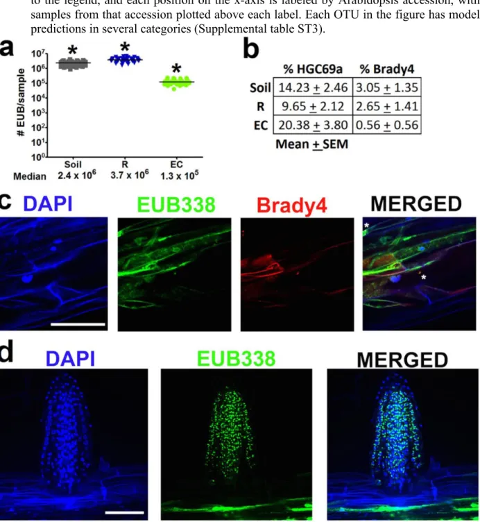
Figure 2.4 CARD–FISH confirmation of Actinobacteria on roots. A single set of Mason Farm yng Col-0 roots were fixed and stained using CARD–FISH. DAPI, 49,6-diamidino-2-phenylindole.DoubleCARD–FISH was applied using theEUB338 eubacterial probe (green) and either theNON338 probe (a), which is the nonsense negative control of EUB338, or the HGC69a Actinobacteria probe (b). Inset, twofold enlargement of boxed region. Scale bars, 50mm.
25
confirmed the rare presence on the rhizoplane of Bradyrhizobiaceae (Figure 2.16c), a family with members defined by the GLMM as more abundant in Mason Farm rhizosphere than Mason Farm EC (Figure 2.3f and Figure 2.15f). We enumerated the relative number of CARD–FISH signals on a set of filters made from equal amounts of material harvested in the same way as were the samples processed for pyrotag sequencing (Figure 2.16a, b). We confirmed that Actinobacteria were found in higher abundance, and that Bradyrhizobiaceae were present in lower abundances, in EC samples than in the bulk soil and rhizosphere samples. We also noted that emerging lateral roots were typically heavily colonized by a variety of bacteria (Figure 2.16d) consistent with previous observations (Chi et al. 2005). These results are PCRindependent support for our sequencing methods.
We present a reduced-complexity, robust experimental platform with which to study root microbiota. Our data, and similar conclusions presented in a companion publication (Bulgarelli et al. 2012b) using a similar platform, provide the deepest analysis available regarding the principles of root microbiome assembly for any plant species. Remarkably, our conclusions are very similar to those in (Bulgarelli et al. 2012b) and we identify phyla and family level enrichments in the EC fraction that largely overlap with those reported in (Bulgarelli et al. 2012b). We note three main differences between our study and that of (Bulgarelli et al. 2012b): different soils from a different continent, a different primer pair and a different portion of root harvested (top 3 cm in (Bulgarelli et al. 2012b); whole root here).
26
level of plant–microbe ‘intimacy’ further increases from the external rhizosphere to the intercellular EC. Both common and soil-typespecific OTUs are established inside roots grown in diverse soils. A small number of bacterial taxa, particularly the Actinobacteria family Streptomycetaceae, and several Proteobacteria families, are highly enriched in the EC. Actinobacteria are well known for production of antimicrobial secondary metabolites (Firáková,
Šturdíková, and Múčková 2007), and many proteobacterial families contain plant-growth-promoting members. Conversely, several taxa (Acidobacteria, Verrucomicrobia and Gemmatimonadetes, and various proteobacterial families) that are common in soil and rhizosphere are depleted from the EC. This depletion suggests that these taxa are either actively excluded by the host immune system, outcompeted by more-successful EC colonizers or metabolically unable to colonize the EC niche. Our identification of a limited-diversity EC facilitates detailed characterization of the isolates comprising the core A. thaliana microbiome, which could facilitate the design of community-based plant probiotics.
27
associations in particular soils may signal interactions that meet environment-specific host needs, balancing contributions of EC microbiome and host genome variation to overall metagenome function. These two generalities suggest that the A. thaliana root microbiome might assemble by core ecological principles similar to those shaping the mammalian microbiome, in which core phylum level enterotypes provide broad metabolic potential combined with modest levels of host-genotype-dependent associations that individualize the metagenome (Arumugam et al. 2011; Spor, Koren, and Ley 2011). Isolation and characterization of the microbes that define host-genotype-dependent associations, and characterization beyond the 16S gene, should be particularly instructive in unravelling the molecular rules contributing to endophytic colonization and persistence.
2.4 Methods
2.4.1 General strategy
28
layer of soil covering the outer surface of the root system that could be washed from roots in a buffer/detergent solution), and EC (bacteria from within the plant root system after sonication-based removal of the rhizoplane; Figure 2.5). We also collected control soil samples (soil treated in parallel, but without a plant grown in it).
2.4.2 Soil collection and analysis
For each full-factorial experiment, the top 8 in of earth were collected with a shovel and transported to the lab in closed plastic containers at room temperature from two collection sites. The first collection site, Mason Farm, is managed by the North Carolina Botanical Garden and is free of pesticide use and heavy human traffic and is located in Chapel Hill, North Carolina, USA (+35° 53′ 30.40′′, −79° 1′ 5.37′′). The second collection site is the Central Crops Research Station in Clayton, North Carolina, USA (+35° 39′ 59.22′′, −78° 29′ 35.69′′) and is also free of pesticide use. Visible weeds, twigs, worms, insects and so on were removed with gloves, and the soil was then crushed with an aluminium mallet to a fine consistency and sifted through a sterile 2-mm sieve. Because sieved soil from Mason Farm drained poorly and test plants grown in it suffered from hypoxia, we adopted the practice of mixing sterile (autoclaved) playground sand into both Mason Farm (MF) and Clayton (CL) soils at a soil:sand ratio of 2:1. Soil micronutrient analysis was performed on pure and 2:1 mixed soils by the University of Wisconsin soil testing labs.
2.4.3 Seed sterilization and germination
29
one week, then germinated at 24 °C under 18 h of light for one week. Seed coat sterility was confirmed by lack of visible contamination on MS plates during germination, and also by absence of visible contamination after plating some of the whole seeds on KB, 1/10-strength LB and 1/10-strength‘869’ bacterial growth media.
To address whether there were seed-borne microbes that might survive surface sterilization, one-week-old seedlings were taken from sterile MS plates and homogenized by aseptic bead beating under non-bacteriolytic conditions (three 3-mm glass balls per 2-ml tube, with 300-µl PBS, using a FastPrep from MP Bio at speed 4.0 m s−1 for 10 s). The homogenate was streaked onto 1/10-strength LB, 1/10-strength ‘869’ and KB media. No colonies were observed. To detect potential unculturable microbes, we pyrosequenced 16S amplicons from the same homogenates using bacteriolytic DNA preps from the genotypes Col-0, Cvi-0, Sha-0 and Tsu-0 (Figure 2.17). Each accession was individually barcoded and sequenced with 1114F and 1392R, yielding 21,935, 20,747, 23,141 and 20,272 reads, respectively. A matching number of total reads was sampled from each accession using pooled data from the full experimental data set for comparative analysis. Thus, 86,095 high-quality reads were obtained from both non-sterile plants and non-sterile plants, the majority of which were chloroplast sequences. See Figure 2.17 for results.
2.4.4 Seedling growth
30
shower of distilled water (non-sterile) as an accessible proxy for rain water that avoids chlorine and other tapwater additives. Pots were spatially randomized and placed in growth chambers providing short days of 8 h light (800–1,000 lx) at 21 °C and 16 h dark at 18 °C. The use of short days was to help synchronize flowering time between A. thaliana genotypes and to facilitate robust rosette and root growth. After harvesting the floral transition developmental stage, remaining plants and bulk soils were moved from the growth chamber to 16-h days in the greenhouse to promote a more synchronized flowering and senescence for the senescent developmental stage.
2.4.5 Harvesting
Each plant was killed and harvested at one of two developmental time points: (1) at the floral transition and (2) after fruiting when senescence is well underway. We considered the floral transition to have begun when the shoot apical meristem was first apparent in five or more plants. Cvi-0, Sha-0 and Ct-1 occasionally flowered one to two weeks earlier under our conditions than the other A. thaliana genotypes. The senescence harvest began when five or more plants showed 50% or more yellow and/or brown rosette leaves(LEVEY and WINGLER 2005); this occurred approximately four to five weeks after transfer to the greenhouse. Senescence occurred in the same order as bolting (flowering).
31
The aboveground plant organs were aseptically removed. Loose soil was manually removed from the roots by kneading and shaking with sterile gloves (sprayed with 70% EtOH) and by patting roots with a sterile (flamed) metal spatula—this ‘neighbouring soil’ fell to the sterile (flamed) work surface. We followed the established convention of defining rhizosphere soil as extending up to 1 mm from the root surface (Elsas, Trevors, and Starodub 1988) and we removed loose soil on all root surfaces until remaining aggregates were within this range. Roots were placed in a clean and sterile 50-ml tube containing 25 ml phosphate buffer (per litre: 6.33 g of NaH2PO4·H2O, 16.5g of Na2HPO4·7H2O, 200 µl Silwet L-77). Tubes were vortexed at
maximum speed for 15 s, which released most of the rhizosphere soil from the roots and turned the water turbid. The turbid solution was then filtered through a 100-µm nylon mesh cell strainer into a new 50-ml tube to remove broken plant parts and large sediment. The roots were transferred from the empty tube to a new sterile 50-ml tube with 25-ml sterile phosphate buffer, and the turbid filtrate was centrifuged for 15 min at 3,200g to form a pellet containing fine sediment and microorganisms.
32
physical removal of surface microbes by sonication instead of killing them with bleach because sequencing measures DNA; at lower concentrations, bleach kills microbes without necessarily destroying the DNA. Although an extended bleach treatment would also destroy unwanted DNA, it could also enter roots and destroy DNA of interest.
After sonication, the roots were snap-frozen, freeze-dried to remove ice and then stored at
−80 °C until processing. Our rhizosphere and EC fractions were collected using time-practical protocols designed to partition sequencing-quality DNA and may differ slightly from classic definitions of these fractions that rely on partitioning culturable bacteria. We note that sonication may leave some rhizoplane microbes behind, especially if they are in a microniche shielded from the ultrasound. Such artefacts may cause our collected fractions to differ from theoretical definitions.
2.4.6 DNA extraction
pre-33
homogenization that allowed us to prepare some EC samples using the MoBio kit. A comparison of Col-0 fractions soil, rhizosphere and EC across four soil digs of MF, where EC was prepared using MoBio in two digs and MoBio in the other two digs, shows that although we cannot rule out a slight kit effect, both kits produce highly similar clustering separating EC from rhizosphere and soil fractions (Figure 2.9, replicates 3 and 4). DNA quantity was assessed with the Quant-iT PicoGreen dsDNA Assay Kit (Invitrogen) and a plate fluorospectrometer.
2.4.7 PCR
For each 1114F-barcoded 1392R primer set, PCR reactions with ~10 ng of template were performed in triplicate along with a negative control to reveal contamination. The PCR program used was 95 °C for 3 min followed by 30 cycles each of 95 °C for 30 s, 55 °C for 45 s and 72 °C for 1 min, followed by 72 °C for 10 min and then cooling to 16 °C. We first verified that the no-template control did not contain DNA via gel electrophoresis, and then pooled the three replicate PCR products and quantified DNA from each pool with PicoGreen (Invitrogen). Pooled PCR products from 30–48 barcoded samples were then combined in equimolar ratios into a master DNA pool, which was cleaned with Mo-Bio UltraClean PCR Clean-Up kit before submission for standard JGI pyrosequencing using a half-plate of Roche 454-FLX with titanium reagents.
2.4.8 454 pyrotag sequencing
34
isopropanol, DNA-carrying beads were enriched and the enriched beads were loaded on the instrument for sequencing. During the emPCR protocol, we reduced the amplification primer amount from 460 µl in the standard protocol to 58 µl per emulsion cup. This is the same amount of primer used for the paired-end emPCR protocol. One-and-three-quarter million beads were loaded in each plate region (reduced from 2,000,000 beads per region in the standard protocol). A detailed standard protocol is available on request.
2.4.9 Primer test and technical reproducibility
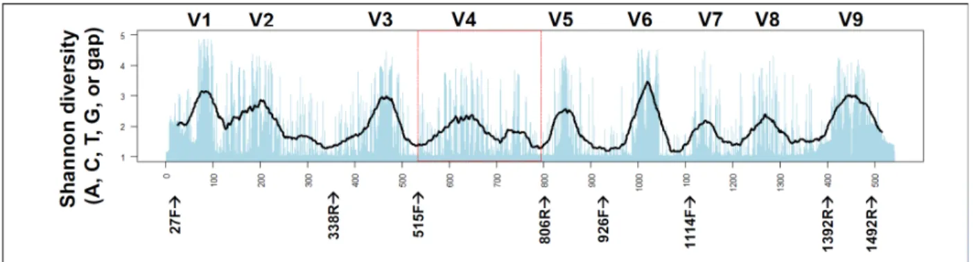
We first tested three sets of broad-specificity 16S rRNA 5′ primers (Jones and Dangl 2006) (Figure 2.6a,b) and established technical reproducibility metrics. We used 13 samples chosen from each of the three sample fractions (soil, rhizosphere and EC) and both soil types (MF and CL) (Figure 2.6c). Each sample was amplified individually with each of the forward primers (804F, which broadly targets bacteria and archaea; 926F, a universal primer; and 1114F, which broadly targets bacteria), paired with the barcoded universal reverse primer (1392R) and sequenced twice to measure technical reproducibility. We identified bacteria by grouping highly similar (97% identity) sequences into OTUs (Supplementary Methods). We chose 1114F for our experiments, on the basis of its broad coverage of the bacterial domain (Lane 1991) and higher usable data yield (Figure 2.6f–i and Figure2.14).
low-35
abundance OTUs are sequentially discarded, was calculated using the software R with a custom script.
2.4.10 Primer specificity sequence
804F prokaryote: 5′-agattagatacccdrgtagt-3′. 926F universal: 5′-actcaaaggaattgacgg-3′. 1114F bacteria: 5′-gcaacgagcgcaaccc-3′.
1392R barcoded universal: 5′-XXXXXacgggcggtgtgtrc-3′. 2.4.11 Sequence processing pipeline and assignment of OTUs
36
The consensus sequence of sequences in each OTU was used as a representative sequence. Each representative sequence was assigned a taxonomy by two methods: (1) using the RDP classifier (Sul et al. 2011) trained on the 4 February 2011 Greengenes reference sequences and (2) by assigning the Greengenes (DeSantis et al. 2006) taxonomy of the best BLAST hit within a combined database including the complete Greengenes 16S database and 18S A. thaliana sequences from NCBI. By the BLAST-based method, sequences without a hit below the E-value threshold of 0.001 are considered unclassified.
Once OTUs were assigned a taxonomy, all OTUs annotated as chloroplasts, Viridiplantae or Archaea on any of the taxonomies were removed from the OTU table, resulting in the set of usable OTUs.
We pooled usable reads from each bulk soil and rarefied to 200,000 reads per soil; this was permuted 100 times. We observed a median of 9,709 OTUs in MF soil and 9,897 OTUs in CL soil. Rarefaction curves to 200,000 reads in each bulk soil (not shown) indicated that, even at 200,000 reads, we were not capturing the entire community in either soil. Consequently, the total number of OTUs we report for our bulk soils may be lower than that found in some reports aimed at finding the true microbial diversity in soils.
37
The frequency table was made from the unnormalized usable OTU table by dividing the number of reads for each OTU in a given sample by the total number of reads in that sample and multiplying by 100, and repeating this across all samples.
We also created a rarefied table; because some samples, particularly samples from the EC, had fewer than 1,000 usable reads in the unnormalized usable OTU table, counts from independent samples sharing the same soil type, genotype, fraction, age and experiment were pooled to make groups of at least 1,000 reads, and the sample names were changed to reflect the pooling that had taken place (Rarefaction_MappingFile… in Supplementary Database 1). Then all samples were rarefied to 1,000 counts using the rrarefy() function in the vegan package of R (Oksanen et al. 2010).
We present both methods because each has advantages and limitations. The advantage of the frequency table is that it keeps each individual plant separate, contains more individual samples and uses all of the data, but this comes at the cost of increased granularity in the normalized relative abundance percentages for some of the samples with fewer reads, causing problems with direct comparability. The major advantage of the rarefied table is that comparisons are not biased by sampling depth and all read counts have equal weight, but this comes at the cost of reduced sample number and samples that mix information from several replicated individuals because we needed to pool some of our samples to meet our rarefaction threshold, and also at the cost of higher overall granularity because we discarded many reads from more deeply sequenced samples.
38
the majority of analyses (the major exception being the UniFrac analysis in Fig. 1: weighted UniFrac distance is robust to rare OTUs). An OTU was deemed measurable if and only if there were ≥ 25 reads in ≥ 5 samples in the unnormalized usable OTU table. As described in the text and Figure 2.6, this threshold was derived from the fact that the correlation between abundance in the same OTU in technical replicates improved greatly as OTUs approached an abundance of 25 reads, and from the fact that although contamination might create an OTU at this abundance once, the probability of an OTU being spurious decreases greatly if it occurs at a measurable level in several (we chose ≥ 5) independent samples.
2.4.12 Detection of differentially enriched OTUs by the GLMM
The OTU abundances were analysed with a GLMM to estimate the effect of the different variables on each measurable OTU. The lme4 R package (Bates, Maechler, and Bolker 2011) was used to fit the model. The abundance of each OTU on each sample (yij) was log2
-transformed and modelled as a function of the abundance of the same OTU in bulk soil samples (std_check) as a fixed effect, and plant genotype (b1), sample type (plant or bulk soil, b2), plant
developmental stage (b3), soil type (b4), sequencing half-plate (b5) and biological replicate (b6)
were modelled as random effects. The full model is specified by
1 2 3 4 5 6
c std_ heck
ij bij bij bij bij bij bij eij
y =β× + + + + + + +
where eij is the residual error and std_check was calculated as the mean abundance of each OTU
39
estimated. The same model specification was used independently on both fractions, and for both the frequency and the rarefied tables (see Supplementary Methods on sequence processing pipeline). The percentage of total variance explained by each random variable on the OTU abundances is reported in Supplementary Table 5.
For each level of the random effects, the conditional mode and 95% prediction interval were estimated by Markov chain Monte Carlo sampling from the fitted model. A specific level is considered to have an effect on an OTU if the prediction interval of its conditional mode does not include zero. OTUs detected this way are reported in Supplementary Database 3.
2.4.13 Partial GLMM
There were not enough samples to estimate all the interaction effect between all variables without drastically reducing the size of the data set and our statistical power (Supplementary Table 2). To assess specific interactions of the genotype effect with other variables, a constrained version of the previously defined GLMM was used that employed only the fixed effect (std_check) and the random effects for plant genotype (b1) and sample type (b2). Samples were
40
2.4.14 Scanning electron microscopy sample preparation
Arabidopsis roots were fixed in 2% paraformaldehyde, 2.5% glutaraldehyde and 0.15 M sodium phosphate buffer, pH 7.4. The samples were dehydrated using a gradual ethanol series (30%, 50%, 75%, 100%, 100%) and dried in a Samdri-795 supercritical dryer using carbon dioxide as the transitional solvent (Tousimis Research Corporation). Roots were mounted on aluminium planchets with double-sided carbon adhesive and coated with 10 nm of gold– palladium alloy (60:40 Au:Pd, Hummer X Sputter Coater, Anatech USA). Images were made using a Zeiss Supra 25 FESEM operating at 5 kV and a working distance of 5 mm, and with a 10-µm aperture (Carl Zeiss SMT Inc.), at the Microscopy Services Laboratory, Pathology and Laboratory Medicine, UNC at Chapel Hill.
2.4.15 Heat maps
Heat maps were constructed using custom scripts and the function heatmap.2 from the R package gplots (Warnes 2011). For better visualization, all data was log2-transformed (per mille:
log2(1,000x + 1)). Hierarchical clustering of rows and columns in the heat maps is based on
Bray–Curtis similarities and uses group-average linkage. 2.4.16 Diversity
41 2.4.17 Rarefaction curves
Rarefaction curves were made with custom scripts that sampled each sample fraction only once at each read depth. To reveal the variance in sampling, no attempt was made to smooth the curves by taking the average of repeated samplings.
2.4.18 Taxonomy histograms and statistics
Taxonomy histograms were created using custom scripts and visualized in GraphPad PRISM version 5.0 for Windows (Motulsky 2003) (GraphPad Software, Inc.; http://www.graphpad.com). The ‘low-abundance’ category was created to help remove visual clutter, and contained any taxonomic group that did not reach at least 5% in any one fraction. The Shannon diversity index was calculated as described above. Differences in distribution at varying taxonomic levels, and differences in Shannon diversity between soil, rhizosphere and EC fractions, were tested by weighted analysis of variance (to account for differing numbers of soil, rhizosphere and EC samples), invoking the central limit theorem (>60 samples in each group in all tests for both frequency-normalized and rarefaction-normalized tests). For more details about tests, see additional notation in Supplementary Table 5.
2.4.19 Sample clustering using UniFrac
42
occupy different major branches on the shared phylogenetic tree of OTUs, whereas samples containing highly similar OTUs will share these major branches. In weighted UniFrac, the branch length unique to each sample is multiplied by the frequency at which that OTU occurs in the sample. Thus, weighted UniFrac can detect differences between two samples that have the same set of OTUs that differ quantitatively between the samples.
Principal coordinate analysis was performed using pairwise, normalized, weighted UniFrac distances between all samples on the unthresholded but normalized OTU tables, and the first two principal coordinates of UniFrac were visualized with GraphPad PRISM version 5.0 for Windows.
2.4.20 CARD–FISH application to roots
We applied a modified protocol described previously (Eickhorst and Tippkötter 2008). Briefly, several root systems from a bolting Col-0 grown in MF were fixed using 4% formaldehyde in PBS at 4 °C for 3 h, washed twice in PBS and stored in 1:1 PBS:molecular-grade ethanol at −20 °C. Treatments with lysozyme solution (1 h at 37 °C, 10 mg ml−1; Fluka) and achromopeptidase (30 min at 37 °C, 60 U ml−1; Sigma) were sequentially used for prokaryotic cell-wall permeabilization. Endogenous peroxidases were inactivated with methanol treatment amended by 0.15% H2O2 at room temperature for 30 min and washed again. Probes
43
formamide concentration, and hybridized at 35 °C for 2 h. Unbound probes were washed away from samples in wash buffer (NaCl content adjusted according to the formamide concentration in the hybridization buffer) at 37 °C for 30 min. Fluorescently labelled tyramide was used for signal amplification, and samples were washed before mounting on glass slides.
For double CARD–FISH, a subset of samples went through a second round of the protocol, starting at the peroxidase inhibition with a second variety of fluorescently labelled tyramide used to be able to distinguish the signals from each probe. Roots were mounted on glass slides using Vectashield with DAPI (Vector Laboratories, catalogue no. H-1200) for mounting solution, and sealed with nail polish for storage. All microscopy images were made on a confocal laser scanning microscope (Zeiss LSM 710 META) located in the Biology Department at UNC. The Brady4 probe, which has not been used for this application previously, was tested on filters of cultured Bradyrhizobiaceae and three negative control cultured strains to determine the most specific formamide concentration in the hybridization buffer.
44
Bradyrhizobiaceae signals were counted as positive when the HGC69a or Brady4 probe co-localized with both EUB338 and the DAPI signal.
2.4.21 Sample naming in OTU tables
All sample names in OTU tables are in the following form: [soil type].[genotype].[sample number][fraction].[age].[experiment]_[plate]. For example, M21.Col.6E.old.M1_2b should be interpreted as [soil type] = M21 = Mason Farm 2:1, [genotype] = Col = Col-0, [sample number] = 6, [fraction] = E = endophyte compartment, [age] = old, [experiment] = M1 = Mason Farm replicate 1, [plate] = 2b.
45 2.5 Supplemental Figures
46
47
considered (red line) the R2 is acceptable at 0.87, a balance between reproducibility and data loss for low-abundance OTUs. In f-i, green circles are EC samples, blue triangles are R samples, and black squares are bulk soil samples. f) Total reads obtained from amplicons made with 804F, 926F, or 1114F paired with bar-coded 1392R. g) Percent of the ‘usable’ reads from f which are not identified as plant or chimeric OTUs. h) Shannon-Weiner species diversity of 1000 usable reads (for each sample with ≥1000 reads). i) Chao1 diversity of 1000 usable reads from each sample (for each sample with ≥1000).
48
49
Shannon diversity of individual samples from each fraction, calculated from the rarefaction-normalized table, before (left) and after (right) applying the 25x5 measurable OTU threshold.
50
51
52
53
54
Figure 2.12 Overlap of GLMM predictions between rarefaction-normalized and
55
56
57
58
59
bar; some may not be visible because they are at 0. In i and j, sample color is according to the legend, and each position on the x-axis is labeled by Arabidopsis accession, with samples from that accession plotted above each label. Each OTU in the figure has model predictions in several categories (Supplemental table ST3).
60
statistical significance at p<1x10¹⁶ (ANOVA with post-hoc TukeyHSD) between each of the sample groups (b) Using double CARD-FISH on filters made from equal concentration of the 3 sample fractions, we determined the % of DAPI positive eubacteria that are also co-localize with either the HGC69a (Actinobacteria) or Brady4 (Bradyrhizobiaceae) probes on filters made from bulk soil (n=10), rhizosphere (n=10), and endophytic compartment (n=10) samples. Actinobacteria was in higher abundance in EC samples and Bradyrhizobiaceae was in lower abundance in EC samples compared to soil and R samples as expected from our pyrotag sequencing data. (c) Double CARD-FISH was applied using the EUB338, eubacterial probe (green) and the Brady4, Bradyrhizobiaceae probe (red), counterstained with DAPI (the asterisks indicate signals that are positive in all 3 channels). (d) Newly forming lateral roots and root tips were found commonly to be heavily colonized. Scale bars represent 50 microns
.
61
86095 HQ reads obtained from both sterile plants and non-sterile plants, the majority were from chloroplast OTUs (not shown). Far more non-plant reads were obtained from the non-sterile plants (19093 of 86095, or 22%) vs. sterile plants (34 of 86095, or 0.04%), a difference approaching three orders of magnitude. The 34 reads from non-sterile plants were members of 31 OTUs (triangles – some overlap on the log-scale axis). No OTU in a sterile plant sample was represented by more than one read, and only two OTUs were shared by more than one of the accessions - both of these shared OTUs were not in the measurable set, and had poor taxonomic classification. 11 of these 31 OTUs were not represented in the non-sterile samples. Furthermore, by including extra unused barcodes in our mapping files, or by sequencing sterile water in excess, we have been able to
62
63
plot. The top panel is based on rarefied data, as in Figure 2.3, and the bottom panel is based on the relative abundance, as in Figure 2.15. (Note: ‘a’ and ‘b’ in our plate naming scheme do not represent different regions of the same plate. All 454 regions were
modeled independently in the Full GLMM).
Figure 2.19 Phyla in each sample fraction by soil type. Histogram displaying the
distribution of the phyla present in the 778 measurable OTUs in soil (S), rhizosphere (R) and endophytic compartments (EC) with each soil type, MF and CL, considered
64
CHAPTER 3: PRACTICAL INOVATIONS FOR HIGH-THROUGHPUT AMPLICON
SEQUENCING2
3.1 Overview
We describe improvements for sequencing 16S ribosomal RNA (rRNA) amplicons, a cornerstone technique in metagenomics. Through unique tagging of template molecules before PCR, amplicon sequences can be mapped to their original templates to correct amplification bias and sequencing error with software we provide. PCR clamps block amplification of contaminating sequences from a eukaryotic host, thereby substantially enriching microbial sequences without introducing bias.
3.2 Introduction
Microbes profoundly affect biological processes across Earth’s ecological niches and are frequently identified through culture-independent methods using DNA purified directly from environmental sample (C. A. Lozupone and Knight 2007). Common PCR-based approaches target highly conserved rRNA genes, such as those encoding the 16S/18S and 28S subunits or the internal transcribed spacer (ITS) between them. These ubiquitous genes have diverged enough that polymorphisms across their ‘hypervariable regions’ (Figure 3.4) allow taxonomic classification. Amplicon sequencing is an important and widely used tool for inferring the presence of taxonomic groups in microbial communities, but poor estimates result from
2
65
sequencing errors and biases introduced during amplification. Inefficiencies also result from the amplification of nontarget DNA. Here we describe methods that make rRNA amplicon sequencing more accurate and cost-effective.
3.3 Results
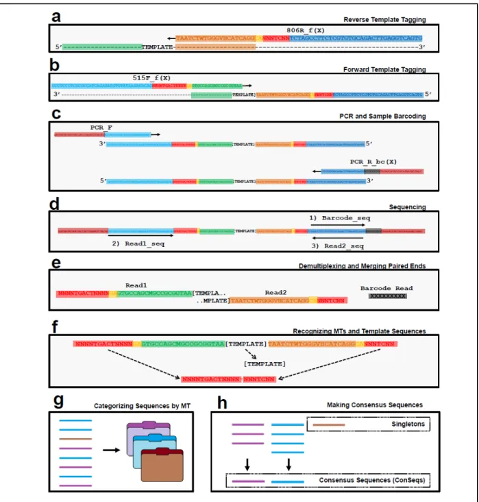
Accurate base-calling on Illumina platforms requires sequence diversity at each nucleotide position (Krueger, Andrews, and Osborne 2011). Because amplicon libraries often lack diversity at specific positions owing to sequence conservation, it is common to spike sequencing runs with sheared genomic DNA from the virus phiX174. We created sequence diversity in 16S amplicons using a mix of primers that have frameshifting nucleotides (Figures 3.5 and 3.6). Despite recent upgrades to Illumina’s base-calling procedure, this strategy remains useful for maximizing data yield as it devotes the entire sequencing effort to the amplicon of interest (Figures 3.7 and 3.8).
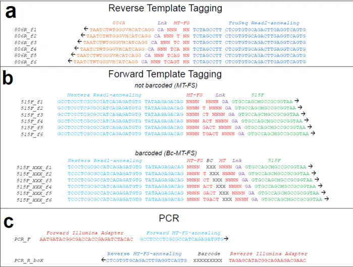
PCR and sequencing introduce sequence errors and sampling bias (Patin et al. 2013). We adapted and validated a modified protocol that uniquely tags each template molecule with random nucleotides before PCR4–7 (Figures 3.5 and 3.9a,b). Provided that there are enough random nucleotides, amplicons sharing the same tag are overwhelmingly likely to have originated from the same template molecule (the ‘birthday paradox’8; Figure 3.10). Thus, by generating consensus sequences from each group of sequences sharing a molecule tag (MT), we can correct errors and infer the amplicon’s probable template sequence (Figure 3.9f–h).
66
had fivefold lower mean error than a sample of 15,000 untreated (nonconsensus) 16S sequences (Fig. 1b and Online Methods).