Chung_unc_0153D_16021.pdf

(1)

STATISTICAL CONTRIBUTIONS TO ORDER RESTRICTED INFERENCE FOR SURVIVAL DATA ANALYSIS

Yunro Chung

A dissertation submitted to the faculty at the University of North Carolina at Chapel Hill in partial fulfillment of the requirements for the degree of Doctor of Philosophy in

the Department of Biostatistics in the Gillings School of Global Public Health.

Chapel Hill 2016

(2)

c ○ 2016 Yunro Chung

(3)

ABSTRACT

Yunro Chung: Statistical Contributions to Order Restricted Inference for Survival Data Analysis

(Under the direction of Jason P. Fine and Anastasia Ivanova)

This dissertation aims to study order restricted inference for survival data analysis where a hazard function is assumed to have a shape restriction with respect to continuous covariates.

In the first chapter, we consider estimation of the semiparametric proportional haz-ards model with a completely unspecified baseline hazard function where the effect of a continuous covariate is assumed isotonic (or monotone) but otherwise unspecified. The pseudo iterative convex minorant algorithm is proposed to compute the isotonic estima-tor by optimizing a sequence of pseudo partial likelihood functions. A local consistency is established for a one-step update of the estimator when an initial value is in a shrinking neighborhood of the true value. Analysis of data from a recent HIV prevention study illustrates the practical utility of the methodology in estimating monotonic covariate effects that are nonlinear.

In the second chapter, we consider additive hazards model with a unimodal hazard function in a continuous covariate with unknown mode. A quadratic loss function is defined, which allows efficient computations to estimate the mode and unimodal covariate effects. The methodology is applied to analyze the data from a recent randomized clinical trial of cardiovascular disease in kidney transplant patients.

(4)

(5)

TABLE OF CONTENTS

LIST OF TABLES . . . ix

LIST OF FIGURES. . . x

CHAPTER 1 : INTRODUCTION. . . 1

Isotonic Hazard Function of a Univariate Continuous Covariate . . . 1

Unimodal Hazard Function of a Univariate Continuous Covariate . . . 2

Isotonic Hazard Function of Multiple Continuous Covariates . . . 2

CHAPTER 2 : LITERATURE REVIEW . . . 4

Order Restricted Inference. . . 4

Constrained Full-likelihood Approach . . . 4

Monotone Response Model with Constrained and Unconstrained Estimators. 5 Non-separable Likelihood Frameworks . . . 7

Computational Algorithms for Order Restricted Inference . . . 8

Iterative Convex Minorant Algorithm for the Case 2 Interval Censored Model . . . 9

Profiling Algorithm for Unimodal Regression . . . 10

(6)

CHAPTER 3 : PARTIAL LIKELIHOOD ESTIMATION OF ISOTONIC

PROPORTIONAL HAZARDS MODELS. . . 13

Introduction . . . 13

Constrained partial likelihood estimation . . . 16

Iterative quadratic programming and iterative convex minorant algorithm without censoring . . . 16

Pseudo iterative convex minorant algorithms with no censoring . . . 19

Censoring . . . 21

Time-dependent covariate . . . 23

Local consistency of the pseudo partial likelihood estimator . . . 24

Extensions . . . 27

Baseline hazard function . . . 27

Additional covariates . . . 27

Simulations . . . 29

HIV data. . . 31

Discussion . . . 35

Technical Details for Chapter 3 . . . 37

CHAPTER 4 : SHAPE RESTRICTED ADDITIVE HAZARD MOD-ELS: MONOTONE, UNIMODAL AND U-SHAPE HAZ-ARD FUNCTIONS . . . 47

Shape restricted additive hazard model . . . 49

Data set-up and loss function . . . 49

(7)

Quadratic pool-adjacent-violators algorithm with no censoring . . . 53

Censoring . . . 55

Time-dependent covariates . . . 56

Extension . . . 58

Monotone and U-shape hazard functions . . . 58

Simulations . . . 60

Folic acid for vascular outcome reduction in transplantation study . . . 62

CHAPTER 5 : ADDITIVE ISOTONIC PROPORTIONAL HAZARDS MODELS. . . 75

Additive isotonic proportional hazards models . . . 77

Data set-up and partial likelihood . . . 77

Cyclic optimization . . . 78

Univariate optimization without censoring . . . 79

Censoring . . . 81

Time-dependent covariates . . . 82

Extension . . . 83

(8)

Data analysis . . . 86

CHAPTER 6 : SUMMARY AND FUTURE RESEARCH . . . 92

(9)

LIST OF TABLES

Table 3.1 Simulation results for time independent covari-ates: IMSE multiplied by103(median CPU time in sec-onds), convergence percentage and matched case per-centage. The first and second lines are for anchor

points ofK =0⋅5 and K =0respectively. . . 32 Table 3.2 Simulation results for time-dependent covariates:

IMSE multiplied by103(median CPU time in seconds), convergence percentage and matched case percentage. The first and second lines are for anchor points ofK =

0⋅5 and K =0 respectively. . . 33 Table 4.1 Simulation results for time independent

covari-ate: IMSE multiplied by 105 (CPU time in seconds), bias multiplied by 103 and MSE multiplied by ₁₀3 for known and unknown modes, where φ1 = −∣Z −M∣,

φ2= −∣Z−M∣1/2 and φ₃ = −∣Z−M∣2. . . 63 Table 4.2 Simulation results for time-dependent covariate:

IMSE multiplied by 105 (CPU time in seconds), bias multiplied by103and MSE multiplied by₁₀3 for known and unknown modes, where φ1 = −∣Z(t) −M∣, φ₂ =

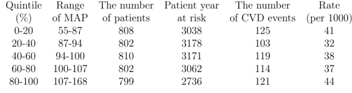
−∣Z(t) −M∣1/2 and φ₃= −∣Z(t) −M∣2. . . 64 Table 4.3 Rate of CVD events by quantiles. . . 66

Table 5.1 Simulation results for time independent covari-ates: IMSE multiplied by 105, CPU time in seconds

and convergence percentage. . . 86 Table 5.2 Simulation results for time-dependent covariates:

IMSE multiplied by105, CPU time in seconds and

(10)

LIST OF FIGURES

Figure 3.1 The Breastfeeding, Antiretroviral and Nutrition study. Estimated hazard ratios based on the isotonic partial likelihood estimator (black solid) and standard proportional hazards models with polynomials of order one (grey solid), two (dashed) and three (dot-dashed). The reference group is CD4 count equal to 200. The

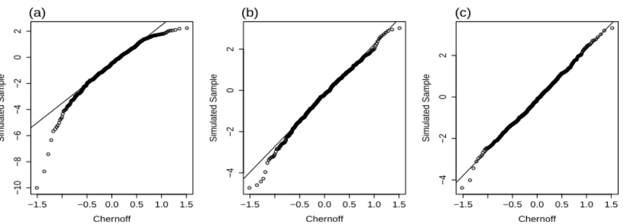
circles indicate HIV infections. . . 35 Figure 3.2 Quantile-quantile plot of simulated sample

ver-sus Chernoff’s distribution atz0 =0⋅1 with no censoring

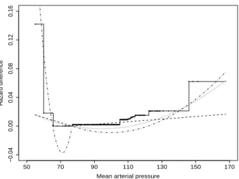
and ψ(z) =z. (a)n=100; (b) n=500; (c) n=1000. . . 36 Figure 4.1 FAVORIT study: U-shape (black solid) versus

standard additive hazards models with polynomials of degree 2 (grey solid), piecewise linear (dashed), piece-wise polynomials of degree 2 (dot-dashed). The black

dots indicate CVD events. . . 67 Figure 5.1 FAVORIT study: Estimated hazard ratios.

Uni-variate isotonic proportional hazards model (black solid), additive isotonic proportional hazards model (dashed) and standard additive proportional hazards mode with polynomials of 1 (grey solid) and 2 (dot dashed). Left is for systolic blood pressure. Right is for age. The

(11)

CHAPTER 1: INTRODUCTION

1.1 Isotonic Hazard Function of a Univariate Continuous Covariate

(12)

1.2 Unimodal Hazard Function of a Univariate Continuous Covariate

We next focus on a unimodal function, where the hazard function is non-decreasing and non-increasing on(−∞, M]and[M,+∞), respectively. The pointM is called a mode, which is generally unknown. We consider the unimodal regression approach (Shoung and Zhang 2001) that estimated unimodal functions at each hypothetical mode and estimated the mode to be the value at which the least square function had a minimum value. His profiling algorithm is directly applicable to the popular proportional hazard model, but there may be a computational challenge owing to the complicated structure of the partial likelihood. Alternatively, we consider estimation of the unimodal hazard function under the semiparametric additive hazard model (Lin and Ying 1994). It defines a quadratic loss function having a global Hessian matrix, which does not involve parameters. Thus, once the global Hessian matrix is computed, a standard quadratic programming method can be performed by profiling the mode.

1.3 Isotonic Hazard Function of Multiple Continuous Covariates

(13)

(14)

CHAPTER 2: LITERATURE REVIEW

2.1 Order Restricted Inference

In this Section, we review literature on order restricted statistical inference based on three types of the likelihood functions: full-likelihood function for bivariate shape re-stricted hazard functions in Subsection 2.1.1, separable likelihood function for monotone response models in Subsection 2.1.2, and non-separable likelihood function for the panel counting data and case 2 interval censored data 2.1.3.

2.1.1 Constrained Full-likelihood Approach

Ancukiewicz et al. (2003) proposed a full-likelihood approach to estimate hazard function under monotonicity. Their model is defined as

λ(t, z) =1− {1−λ₀(t)}f(z),

whereλ0(⋅) is an unspecified baseline hazard function, andf(⋅)is a monotone increasing function. They further assume thatλ0(⋅) has a range in [0,1), and f(⋅) is non-negative. Let t1< ⋯ <t_s be the distinct observed failure times, and let z₁< ⋯ <z_m be the distinct covariate values at any of those observed failure time. The full-likelihood function is then defined as

l(f, λ₀) =

m

∑

i=1

s

∑

j=1

(15)

wheredi,j andni,jare the number of patients at risk and the number failed at timetj with

covariate zi, respectively. They propose an algorithm to maximize the full-likelihood by

updating λ0 given f and updating f given λ0 iteratively until convergence. During the maximization steps, one additional constraint is imposed to have a unique factorization, where∑m_i₌₁f(z)is set to the number of observationn. However, their proposed algorithm was ad hoc and did not have a global or even local convergence property.

2.1.2 Monotone Response Model with Constrained and Unconstrained Es-timators

Banerjee (2007) suggested the monotone response model. Consider independent and identically distributed data {X_i, Z_i}n_i=1, where X_i∣Z_i =z ∼p(x, ψ(z)), p is a probability density, and ψ(⋅) is a monotone increasing (or monotone decreasing) function. One example is the monotone regression model, which is

Xi=ψ(Z_i) +_i,

wherei is independent of Zi with mean 0 and variance σ2. Here, Zi is a covariate value

for the ith subject, and Xi is the response value. By assuming i’s are Gaussian, this

model is expressed as a monotone response, where Xi∣Z_i = z ∼ N(ψ(z), σ2). Another example is the case 1 interval censored model. LetUi andZi be an event and observation

times for the ith subject, respectively, and Xi =1 if U_i ≤Z_i, or X_i =0 otherwise. Here, Ui is independent ofZi. A main goal was to estimate F, a survival function of theUi’s.

It is also expressed as a monotone response model, whereXi∣Z_i=z ∼Bernoulli(F(z)). Let l(X_i, ψ(Z_i)) = −log{p(X_i, ψ(Z_i))}. The negative log-likelihood function for the monotone response model is then defined as

l(x, ψ(z)) =

n

∑

i=1

(16)

Letψi=ψ(Z(i)), whereZ(i)is theith smallest value amongZi’s. LetX(i)be the response value corresponded to Z(i). Denote ψˆ as the minimizer over the monotone constraint that minimizes∑n_i₌₁l(X₍_i₎, ψ_i)subject toψ₁≤ ⋯ ≤ψ_n. Denotel˙and ¨l as first and second derivatives of the negative log-likelihood. It is shown that _ψˆ _{is a minimizer over the}

monotone constraint if and only if

n

∑

j=1

˙

l(X₍_j₎,ψˆ_j) =0

and

n

∑

j=i

˙

l(X(j),ψˆj) ≥0 (i=1,. . . ,n).

By assuming its Hessian matrix is a diagonal and positive define matrix, the minimizer is characterized by

(ψˆ₁, . . . ,ψˆ_n) =slogcm[

i

∑

j=1

¨

l(X₍_j₎,ψˆ_j),

i

∑

j=1

{ψˆ_j¨l(X₍_j₎,ψˆ_j) −l˙(X₍_j₎,ψˆ_j)}]

n

i=0 ,

where ∑0_i₌₀ = 0, and slogcm[x_i, y_i]n_i₌₀ is the vector of slopes (or left derivatives) of the greatest convex minorant on cumulative sum diagram (x_i, y_i)’s.

He further suggested an constrained minimizer _ψˆ0 by minimizing the negative log-likelihood function in (2.2) under the monotone constraint and the null hypothesis, H0∶ ψ(z₀) = θ0. Denote k as the number of Z_i’s that are less than or equal to z0. Since the negative log-likelihood function is separable in terms ofZ(i)’s, the minimization problem can be separated to two minimization problems: minimize ∑k_i₌₁l(X₍_i₎, ψ_i) subject to ψ1 ≤ ⋯ ≤ψ_k ≤θ0, and minimize ∑n_i=k+1l(X(i), ψi) subject to θ0 ≤ψk+1 ≤ ⋯ ≤ψn. Similar to the unconstrained minimizer, the constrained minimizer is characterized by

(ψˆ₁, . . . ,ψˆ_k) =slogcm[

i

∑

j=1

¨

l(X(j),ψˆj),

i

∑

j=1

{ψˆ_j¨l(X(j),ψˆj) −l˙(X(j),ψˆj)}]

n

(17)

and

(ψˆ_k₊₁, . . . ,ψˆ_n) =slogcm[

i

∑

j=1

¨_l₍_X

(j),ψˆj),

i

∑

j=1

{ψˆ_j¨l(X(j),ψˆj) −l˙(X(j),ψˆj)}]

n

i=k ∨θ₀.

Here, ∧ and ∨ are the minimum and maximum operators, respectively. Based on the constrained and unconstrained minimizers, he developed likelihood ratio test.

2.1.3 Non-separable Likelihood Frameworks

The isotonic regression technique has been developed under independent and iden-tically distributed data, where its likelihood function is separable. For example, the full-likelihood function in (2.1) in Subsection 2.1.2 is separable in terms of zi given λ0.

The likelihood function in (2.2) is also separable in terms of Zi in Subsection 2.1.2. The

separable structure allows a relatively easy computation for an isotonic estimator. On the other hand, the following paragraphs describe two recent works for order restricted inference under non-separable likelihood functions, where the non-separation structure is from dependent data.

A first example is the panel count data (Wellner and Zhang 2000), where each subject is observed multiple time points with respect to the counts of events. Let N = {N(t) ∶ t ≥ 0} be a counting process with mean function E(N(t)) = Λ₀(t), K be an integer-valued random variable, and T = {T_k,j, j =1. . . , k, k = 1,2, . . .} is potential observation times. Here, N and (K, T) are independent, and T_k,j₋₁ ≤ T_k,j for j = 1, . . . , k and k =

1,2, . . .. Denote {N_K(i) i, T

(i)

Ki, Ki}

n

i=1 as the independent and identically distributed copies of (N, T, K). By assuming N is a Poisson process that has the independent increment property, the log-likelihood function for Λ is defined as

l(Λ) =

n

∑

i=1 [

Ki

∑

j=1 (N_K(i)

i,j−N

(i)

Ki,j−1)log{Λ(T

(i)

Ki,j) −Λ(T

(i)

Ki,j−1))} −Λ(T

(i)

(18)

which includes only two adjacent parameters at each j. Thus, it is reformulated as

n

∑

i=1 [

Ki

∑

j=1

{∆N_K_i_,jlog(∆Λ_K_i_,j) −∆Λ_K_i_,j}],

where ∆NKi,j = N

(i)

Ki,j−N

(i)

Ki,j−1, and ∆ΛKi,j = Λ(T

(i)

Ki,j) −Λ(T

(i)

Ki,j−1). The reformulated

likelihood function was separable in terms ofj, so that an isotonic regression method for independent data was used to make an inference forΛ.

A second example is the case 2 interval censored data. Let {X_i, T_i, U_i}n_i₌₁ be inde-pendent sample from R3+, where Xi is an event time with distribution function F0, and

Ti and Ui are observation times with a joint distribution H. Here, Xi and (Ti, Ui) are

independent withTi≤U_i. The log-likelihood for F is then defined as

l(F) =

n

∑

i=1

[δ_ilogF(T_i) +γ_ilog{F(U_i) −F(T_i)} + (1−δ_i−γ_i)log{1−F(U_i)}], (2.3)

where δi=I(X_i≤T_i), and γ_i =I(X_i ∈ (T_i, U_i]), and where I(⋅) is the indicator function. The likelihood function is not separable in terms ofTi. However, it is partially separable

in terms of left, right and interval censoring times. This partial separation plays a key role in showing consistency (Groeneboom and Wellner 1992) and asymptotic distributional result (Groeneboom 1996) for the isotonic estimator _Fˆ_.

2.2 Computational Algorithms for Order Restricted Inference

(19)

2.2.1 Iterative Convex Minorant Algorithm for the Case 2 Interval Censored Model

The iterative convex minorant algorithm is suggested to solve the case 2 interval censored data (Groeneboom 1996, pp. 69-73). The fundamental idea of the iterative convex minorant algorithm is that a convex optimization problem is reduce to a series of weight isotonic regression problems. The negative log-likelihood of (2.3) is represented as

ln(F) = −{ ∑

j∈I1

logβj+ ∑

j∈I2a

log(β_k₍_j₎−β_j) + ∑

j∈I3

log(1−β_j)},

where βi =F(ν_i) and k(j) = {k ∶ ν_k = max(U_i, V_i), ν_j =min(U_i, V_i), γ_i = 1, i = 1, . . . , n}, and where I1 = {j ∶ ν_j = U_i with δ_i = 1}, I₂_a = {j ∶ ν_j = min(U_i, V_i) with γ_i = 1} and I3 = {j ∶ ν_j = V_i with δ_i+γ_i = 0} for i = 1, . . . , n and j = 1. . . , l. Here, ν₁ < . . . < ν_l is a sorted set of time points among Ui’s with δi = 1 or γ_i = 1 and V_i’s with γ_i = 1 or δi +γi = 0 and γi = 0 for i = 1, . . . , n. In order to ensure l(F) > ∞, it is assumed

that 1 ∈I₁ and l ∈ I3. The goal is to find the maximizer of l(F) over the convex cone C = {β ∈ _Rl ∶ β₁ ≤ ⋯ ≤ β_l}. Denote l˙n(F) as the first derivative of ln(F). Then, the convex function ln₍_F₎ is approximated locally near_β(0) by a quadratic function

ln(F) ≈

1 2{β−β

(0)

+W(β(0))−1l˙n(β(0))}TW(β(0)){β−β(0)+W(β(0))−1l˙n(β(0))},

whereW is a Hessian matrix. By ignoring off-diagonal elements inW, the approximated quadratic function is reduced to

ln(F) ≈

1 2

n

∑

i=1

{β_i−β_i(0)+w_i(β(0))−1l˙n_i(β(0))}2w_i(β(0)),

(20)

in C, and then, the series of weight isotonic regression functions are solved by using either the greatest convex minorant or pool-adjacent-violators algorithm iteratively until convergence. The convergence criteria is Fenchel’s duality conditions

l

∑

i=1

ˆ

βil˙ni(βˆi) =0

and

l

∑

i=1

βil˙ni(βˆi) ≥0.

for or all (β₁, . . . , β_l) ∈ C. A distance stopping criteria may be alternatively used but it is a weaker condition than Fenchel’s stopping criteria (Wellner and Zhan 1997). An advantage of the iterative convex minorant algorithm is computational speed, since the approximated likelihood function has simpler structure by ignoring the off-diagonal ele-ments in W. At the time when the iterative convex minorant algorithm was suggested, convergence property was not proven. It was conjectured that Fenchel duality conditions did not depend on the Hessian matrix, and the Hessian matrix contained only few nonzero off-diagonal elements. Aragón and Eberly (1992) showed the local convergence under the (unrealistic) assumption where the jump points of the nonparametric maximum likeli-hood estimation are determined prior to applying the algorithm. Later, Jongbloed (1998) modified the iterative convex minorant algorithm to have a global convergence property by adding a line search algorithm.

2.2.2 Profiling Algorithm for Unimodal Regression

We consider the unimodal regression (Shoung and Zhang 2001) that minimizes

LS(f₀) =

n

∑

i=1

(21)

where (X_i, Y_i) are independent and identically distributed sample from (X, Y), i =

1, . . . , n, and f0 is an unknown unimodal function with an unknown mode m0. To esti-mate m0, they suggested nonparametric least squares estimator, which is

ˆ

m0=Xˆ_j, ˆj =arg min

j=1,...,n

[min

f0∈Fj

LS(f₀)], (2.5)

where Fj = {f₀ ∶f₀ is a unimodal function with mode X_j}. Let X₍_i₎ be the ith largest value among (X₁, . . . , X_n), and Y₍_i₎ be the response value associated with X₍_i). Then they separated the minimization problem in (2.4) into two minimization problems:

min m

∑

i=1

{Y(i)−f0(X(i))}

2 _{subject to} _f

0(X₍₁₎) ≤ ⋯ ≤f₀(X(m)) (2.6)

min n

∑

i=m+1

{Y(i)−f0(X(i))}

2 _{subject to} _f

0(X(m+1)) ≥ ⋯ ≥f0(X(n)). (2.7)

The isotonic and anti-isotonic regression techniques can be separately performed on (2.6) and (2.7) with the pool-adjacent-violators algorithm. Let_fˆ₀_,j _{be the estimated unimodal}

function at the mode ofX(j). The profiling algorithm is to estimate the unimodal function

ˆ

f0,j by profiling every hypothetical mode X(j),j =1, . . . , n, and estimate mode by (2.5).

2.2.3 Cycling Algorithm for Additive Isotonic Regression

Bacchetti (1989) extended the isotonic regression model to the additive isotonic model to include multiple covariates. Let Yi and _Xi _{= (}_Xi

1, . . . , Xdi) be response scalar and

covariate vector values for the ith subject, respectively, i = 1, . . . , n, Let X_j(i) be the ith largest value among (X_j1, . . . , X_jn). The additive isotonic model minimizes the least square function

n

∑

i=1

(22)

over the additive isotonic constraint where µj(X_j(1)) ≤ . . . ≤ µ_j(X_j(n)) for j = 1, . . . , d. They suggested the cycling algorithm that updated a univariate isotonic functionµkwhile

holding other isotonic functions (µ₁, . . . , µ_k₋₁, µ_k₊₁, . . . , µ_n) constant. Correspondingly, the least square function in (2.8) is reduced to

n

∑

i=1

{Y˜i−µ_k(X_ki)}2, (2.9)

where _Y˜i ₌_Yi

− ∑d_j₌₁_,j≠kµj(X

i

j). The reduced least square function in (2.9) has a closed

form over the isotonic constraintµk, which can be computed by using the

(23)

CHAPTER 3: PARTIAL LIKELIHOOD ESTIMATION OF ISOTONIC PROPORTIONAL HAZARDS MODELS

3.1 Introduction

In regression analysis, common parametric models, for example, generalized linear models, may employ shape-restrictions on covariate effects, the simplest being that of monotonicity. There is extensive literature on nonparametric isotonic regression models, where the form of a monotone covariate effect is completely unspecified; see Banerjee (2007). Computational and inferential issues have been well studied, particularly for likelihood-based estimation of isotonic generalized linear models, where efficient algo-rithms are available which exploit the geometric properties of the shape-restricted likeli-hood and which facilitate a careful theoretical analysis of the large sample properties of the resulting estimators. Unfortunately, these approaches are not easily generalizable to partial likelihood estimation of the semiparametric isotonic proportional hazards model, owing to the lack of an independent and identically distributed structure of the partial likelihood. In survival data settings, constrained nonparametric maximum likelihood estimation was developed by Ancukiewicz et al. (2003) using ad hoc algorithms. Such algorithms may not even converge to a local maximum, and appear computationally pro-hibitive in large samples. The goal of this paper is theoretically justified computation of isotonic estimators based on partial likelihood in survival data settings.

(24)

monotone in time (Grenander 1956, Marshall and Proschan 1965, Rao 1970, Mukerjee and Wang 1993, Huang and Wellner 1995, Banerjee 2008, Lopuhaä and Nane 2013), including a 2013 Delft University of Technology PhD thesis by G. Nane, where the baseline hazard function is not assumed to be monotone in time. With categorical covariates having regression parameters known to satisfy a monotone ordering, one may post-process un-restricted partial likelihood estimates using the pool-adjacent-violators algorithm (Ayer et al. 1955) to obtain restricted estimators, similar to post-processing of likelihood esti-mators of parametric regression models with categorical covariates. This approach is not applicable with continuous covariates, owing to the fact that unrestricted estimation is not possible at all values of the covariate. Specialized methods are needed.

Suppose that T is a failure time, C is a censoring time and Z is a scalar continuous covariate, where it is assumed that T and C are independent conditionally on Z. Define X=min(T, C)and∆=I(T ≤C), whereI(⋅)is the indicator function. The observed data consist of n independent and identically distributed replicates of (X,∆, Z), denoted by {X_i,∆_i, Z_i} (i=1, . . . , n). The proportional hazards model (Cox 1972) may be specified to incorporate monotone covariate effects, that is,λ(t∣Z) =λ₀(t)exp{φ(Z)}, whereλ₀(t) is an unspecified baseline hazard function and φ(⋅) is a monotone increasing function. In the usual Cox model, the form of φ(⋅) is specified parametrically, for example, using low-order polynomials ofZ. These parameters may then be estimated by maximizing the partial likelihood without imposing further restrictions on the parameters. When φ(⋅) is monotone but otherwise unspecified, care is needed in defining the estimator using the partial likelihood, denoted by

pl(φ) =

n

∏

i=1 ∏

t≥0 {

eφ(Zi)

∑n_j₌₁Yj(t)eφ(Zj)}

dNi(t) ,

(25)

Unlike the usual likelihood based formulation for isotonic linear models (Robertson et al. 1988), the partial likelihood for the isotonic proportional hazards model is a product integral of terms depending on both time and covariate values, where the parameterφ(⋅) only enters the partial likelihood at those covariate values in the dataset. To ensure that estimation is well-defined between those values, we restrict the estimator to be piecewise constant, which yields a unique estimator with potential jumps at the observed Zi’s.

This assumption is similar to that made in isotonic generalized linear models. For right censored data, we show that the estimator jumps only at those covariate values which are associated with observed failure events with ∆i =1; this is made precise in Subsections 3.2.1-3.2.2.

(26)

3.2 Constrained partial likelihood estimation

3.2.1 Iterative quadratic programming and iterative convex minorant algo-rithm without censoring

Define the isotonic estimator ofφ(⋅)to be the maximizer of the partial likelihood under the monotone constraint that φ(Z₍₁₎) ≤ ⋅ ⋅ ⋅ ≤φ(Z₍_n₎), where Z₍_i₎ is theith smallest value amongZ1, . . . , Zn. One must fix one point of the partial likelihood estimator, otherwise

there is no unique maximizer because all ordered sets of {φ(Z₍₁₎) +δ, . . . , φ(Z(n)) +δ} yield the same value of the partial likelihood for any δ. We impose an anchor constraint that φ(K) =δ by prespecifying a constant K in the support of Z prior to the analysis of the data. Under the anchor constraint, the model fitted is

λ(t∣Z) =λ₀(t)eφ(Z)= {λ₀(t)eδ}eψ(Z), (3.1)

whereψ(Z) =φ(Z)−δwithψ(K) =0. Since the baseline hazard function absorbsexp(δ), what we actually estimate is notφ(⋅)butψ(⋅). We regardδas a nuisance parameter, with the only difference between ψ(⋅) and φ(⋅) being the reference group defining the hazard ratio parameters. In other words, ψ(⋅) is vertically shifted from φ(⋅) byδ, where hazard ratios based on ψ(⋅) and φ(⋅) are identical, i.e., exp{φ(⋅) −φ(K)} = exp{ψ(⋅) −ψ(K)}. In practice, since ψ(⋅) is only estimable at the observedZ(i)’s, we setψ(Z(k)) =0, where Z(k) is the largestZ(i)≤K.

Let lN₍_ψ₎ denote the negative log partial likelihood,

lN

(ψ) = ∑n_i₌₁

ˆ ∞

0

[−ψ(i)+log{∑

n

j=1Y(j)(u)e

ψ(j)_}]dN

(i)(u),

(27)

subparentheses for notational convenience. The score function and Hessian matrix of the negative log partial likelihood are denoted asU(ψ)andH(ψ), respectively, with elements

us(ψ) =

∂lN₍_ψ₎

∂ψs

= −

ˆ ∞

0

dNs(u) +

ˆ ∞

0

Es(ψ, u)dN¯(u),

hss(ψ) =

∂2_lN

(ψ) ∂ψ2

s

=

ˆ ∞

0

{E_s(ψ, u) −E_s(ψ, u)2}dN¯(u),

hst(ψ) =

∂2_lN₍_ψ₎

∂ψs∂ψt

= −

ˆ ∞

0

Es(ψ, u)E_t(ψ, u)dN¯(u),

for s, t = 1, . . . , n (s ≠ t), where E_s(ψ, u) = Y_s(u)exp(ψ_s)/{∑n_j₌₁Yj(u)exp(ψ_j)} and dN¯(u) = ∑n_i₌₁dNi(u).

Theorem 3.1. Suppose that there is no censoring. The negative log partial likelihood

lN₍_ψ₎ _{is convex. It is strictly convex when an anchor constraint is imposed that} _ψ

k =

ψ(Z(k)) =0.

Let Ψk be _{_ψ _∈

Rn ∶ ψ₁ ≤ ⋯ ≤ψ_n, ψ_k = 0}. The problem of maximizing the partial likelihood over the monotone and anchor constraints is equivalent to minimizing the strictly convex function lN₍_ψ₎ over the convex cone _Ψk. We denote the minimizer of

lN₍_ψ₎ over _Ψk by _ψˆ _{= (}_ψˆ

1, . . . ,ψˆn), which we refer to as the isotonic partial likelihood estimator.

To uniquely estimate ψ at covariate values other than those in Z(1), . . . , Z(n), we assume, similar to previous work on isotonic regression, that the estimator is a right-continuous step function with jumps at the order statistics of the Zi’s. Under this

as-sumption, the strict convexity in Theorem 3.1 coupled with the following theorem give a unique characterization of the isotonic partial likelihood estimator:

Theorem 3.2. Suppose that there is no censoring. The isotonic partial likelihood

(28)

holds that ψˆ∈Ψk satisfies

∑

i

j=1uj(ψˆ) ≤0 (i=1, . . . , k−1), ∑

n j=iuj(

ˆ

ψ) ≥0 (i=k+1, . . . , n), (3.2) ∑

n i=1,i≠k

ˆ

ψiui(ψˆ) =0. (3.3)

Moreover, ψˆ is uniquely determined by (3.2) and (3.3).

Iterative quadratic programming can be applied to find the isotonic partial likelihood estimator. It is designed to approximate a convex function by a quadratic function and find a solution by minimizing the quadratic function. A second order Taylor series approximation of lN

(ψ)about ψ0 is

lN

(ψ) ≈lN(ψ0) + (ψ−ψ0)U(ψ0) + (ψ−ψ0)H(ψ0)(ψ−ψ0)/2

=

1

2{ψ−ξ(ψ

0

)}H(ψ0){ψ−ξ(ψ0)} +g(ψ0), (3.4)

where ξ(ψ0) =ψ0−H(ψ0)−1U(ψ0), and g(ψ0) =lN(ψ0) −U(ψ0)H(ψ0)−1U(ψ0)/2 which does not depend onψ. The procedure of the iterative quadratic programming method is that we set an initial value ψ(0)_∈_Ψk, and update_ψ(m)

∈Ψk by minimizing the first term in (3.4),{ψ(m)−ξ(ψ(m−1))}H(ψ(m−1)){ψ(m)−ξ(ψ(m−1))}, until convergence. The solution can be found by using a quadratic programming method with equality and inequality constraints. In the simulations reported in Section 3.4, we find that the procedure may be numerically unstable, with convergence dependent on the anchor constraint.

(29)

approximated partial likelihood in (3.4) reduces to

1

2∑

n

i=1{ψi−ξi(ψ 0

)} 2

hii(ψ0) +g(ψ0), (3.5)

where ξi(ψ0) = ψ0_i −u_i(ψ0)/h_ii(ψ0). This is identical to finding a monotone increasing function that minimizes ∑n_i₌₁{ψ_i−ξ_i(ψ0)}2h_ii(ψ0) over the class of monotone increasing functions Ψk with weight _h. One may use the pool-adjacent-violators algorithm to find

the minimizer (Ayer et al. 1955). The procedure of iterative convex minorant algorithm is to set an initial value of ψ(0)_∈_Ψk, and apply the pool-adjacent-violators algorithm to

update ψ(m) until convergence. The convergence criteria is based on Fenchel’s duality condition in Theorem 3.2. It characterizes isotonic estimator _ψˆ_{, and in practice, one}

will check this condition and application of the iterative convex minorant algorithm. To incorporate the anchor constraint, we impose a constraint on iterative convex minorant algorithm (Banerjee 2007), where at each mth step after applying the pool-adjacent-violators algorithm, we set ψ(m)

k =0; ψ

(m)

i =0 if ψ

(m)

i >0 for i=1, . . . , k−1; ψ

(m)

i =0 if

ψ(m)

i < 0 for i =k+1, . . . , n. The iterative convex minorant algorithm with the anchor

constraint may be unstable, which strongly depends on the choice of the anchor point, as shown in the simulation studies in Section 3.4.

3.2.2 Pseudo iterative convex minorant algorithms with no censoring

(30)

constrained pseudo partial likelihood,

lP(ψ∣ν) = ∑n_s₌₁

ˆ ∞

0

{−ψsdNs(u) +E_sP(ψ_s, u∣ν)dN¯(u)}, (3.6)

where EP

s(ψs, u ∣ ν) = Y_s(u)eψs/{∑nj=1Yj(u)eνj} for constants ν₁, . . . , ν_n. The pseudo partial likelihood score function and Hessian matrix are defined as

uP_s(ψ_s∣ν) = −

ˆ ∞

0

dNs(u) +

ˆ ∞

0

E_sP(ψ_s, u∣ν)dN¯(u),

hP

ss(ψs∣ν) =

ˆ ∞

0 EP

s (ψs, u∣ν)dN¯(u) >0, (3.7) hP_st(ψ_s∣ν) =0, s, t=1, . . . , n(s≠t). (3.8)

The anchor constraint is not needed for lP₍_ψ_∣_ν₎ because it is a strictly convex function

by (3.7) and (3.8). Let Ψ = {ψ ∈ _Rn ∶ ψ₁ ≤ ⋯ ≤ ψ_n} be the convex cone obtained by removing the anchor constraint from Ψk. The procedure of pseudo iterative convex

minorant algorithm is

Step 3.1: Set an initial value of _ψ˙(0)_∈_Ψk (or _ψ˙(0)_∈_Ψ). Step 3.2: Update _ψ˙(m) such that _ψ˙(m)

=arg min_ψ_∈ΨlP(ψ∣ν=ψ˙(m−1)).

Step 3.3: Repeat Step 3.2 until convergence under the distance stopping criteria de(ψ˙(m),ψ˙(m−1)) <˙ for small˙>0, whered_e(x, y) = ∑n_i₌₁∣exp(x_i) −exp(y_i)∣.

Step 3.4: Let _ψ¨

i =ψ˙_i(m)−ψ˙(_km) (i=1, . . . , n) such that ψ¨= (ψ¨₁, . . . ,ψ¨_n) ∈Ψk.

Theorem 3.3. The minimizer ψ˙ in Step 3.2 minimizes lP₍_ψ_∣_ν₎_{over the convex cone} _Ψ

if and only if Fenchel’s duality condition holds that

∑

n j=iu

P

(31)

with equality holding if i=1, and

∑

n i=1ψ˙iu

P

i (ψ˙i∣ν) =0. (3.10)

Moreover, ψ˙ is uniquely determined by (3.9) and (3.10).

Theorem 3.4. Suppose thatψˆ+ _minimizes

∑n_i₌₁(ψ_i+−w−1_i ∆i)2w_i over the class of isotonic

functions inΨ, where∆i=

´∞

0 dNi(u)andwi=

´∞

0 [{Yi(u)dN¯(u)}/{∑

n

j=1Yj(u)exp(ν_j)}].

Then, ψ˙= {log(ψˆ₁+), . . . ,log(ψˆ_n+)} is the unique minimizer of lP(ψ∣ν) over Ψ.

In Step 3.2, we are not guaranteed to eventually satisfy the convergence criteria in Step 3.3, i.e., it is possible to construct data sets and choose starting values such that the algorithm will not converge. However, in practice we have found this to be unlikely (see Section 3.4). Moreover, the following theorem indicates that if the algorithm does converge for any ˙, then the estimate ψ¨ converges to the unique minimizer of the constrained partial likelihood in Theorems 3.1 and 3.2 as˙→0. This provides theoretical justification for the pseudo iterative convex minorant algorithm.

Theorem 3.5. Suppose that for any ˙>0, there exists r(˙) such that the pseudo

itera-tive convex minorant algorithm converges at r(˙)th iteration under the distance stopping

criteria de(ψ˙(r(˙)),ψ˙(r(˙)−1)) <˙. Then, as ˙→0, ψ¨= (ψ˙₁(r(˙))−ψ˙_k(r(˙)), . . . ,ψ˙₁(r(˙))−ψ˙_k(r(˙)))

converges to the unique minimizer of lN₍_ψ₎ _over _Ψk_.

3.2.3 Censoring

(32)

with these uncensored subjects. One may view the form of this estimator in line with traditional survival analysis where the estimated survival function jumps only at the observed failure times (Kaplan and Meier 1958). To estimate ψ(⋅) computationally, we suggest replacing a parameter for a censored subject with the parameter for an uncensored subject having covariate value which is closest to that for the censored subject amongst all uncensored subjects having smaller covariate values than the censored subject.

Let n⋆ be the number of subjects with observed failure time of the total _n subjects, and Z⋆

i be their covariate values, i = 1, . . . , n⋆. Define n⋆ disjoint intervals of I

⋆ 1 = (−∞, Z⋆

(1)) ∪ [Z ⋆ (1), Z

⋆ (2)), I

⋆ 2 = [Z

⋆ (2), Z

⋆

(3)), . . . , I ⋆

n⋆= [Z

⋆

(n⋆₎,+∞), whereZ

⋆

(i) is theith order statistic amongst theZ⋆

i’s. We can then construct the replacement parameters algorithm

whereψ(Z_h)is replaced with ψ(Z_i⋆)if Z_h∈I_i⋆ forh=1, . . . , n;i=1, . . . , n⋆. Accordingly, at-risk processes for censored subjects are added to corresponding at-risk processes for observed subjects such that Y⋆

i (t) = ∑h∈RiYh(t), where Ri = {h ∶ Zh ∈I

⋆

i, h= 1, . . . , n}.

The partial likelihood for censored data is then defined by

plC

(ψ⋆) =

n⋆ ∏ i=1 ∏ t≥0 { e ψ⋆ i ∑n ⋆

j=1Yj⋆(t)e ψ⋆

j }

dN⋆

i(t) ,

where ψ⋆

i =ψ(Z

⋆

(i))and N ⋆

i (t) is the counting process corresponding toZ

⋆

(i). We assume that ψj =ψ⋆₁ if Z_j < Z⋆

(1) for j =1, . . . , n, otherwise ψj is not included in pl

C₍_ψ₎. This

enables estimation of ψ(⋅) at all values of Z including the left side of Z₍₁₎⋆ . As stated in Proposition 3.6, the replacement parameters algorithm with plC₍_ψ₎is justified.

Proposition 3.6. Assume that ψj =ψ₁⋆ if Z_j <Z₍₁₎⋆ for j =1, . . . , n. Then the isotonic

partial likelihood estimator has jumps only at Z⋆

i’s, and thus, the unique maximizer of

plC₍_ψ₎ _{is also the unique maximizer of} _pl₍_ψ₎_.

(33)

censored data, so that iterative quadratic programming method, iterative convex mino-rant algorithm, and pseudo iterative convex minomino-rant algorithm are applicable to find the unique maximizer of plC₍_ψ₎.

3.2.4 Time-dependent covariate

Consider this model λ(t∣Z(t)) =λ₀(t)exp[ψ{Z(t)}], where Z(t)is a time-dependent covariate. It is assumed that the monotone increasing function ψ(⋅) does not change over time. Similar to censored data, the fact that the values of the time-dependent covariates prior to the first observed failure time do not contribute to the partial likelihood restricts the form of the isotonic partial likelihood estimator. As stated in Proposition 3.7, the isotonic partial likelihood estimator has jumps at the time-dependent covariate values associated with uncensored subjects only at their failure times. One may use replacement parameters algorithm where the parameters for subjects having their failure times observed are substituted for other parameters in the partial likelihood.

Formally, let n⋆ be the number of subjects with observed failure time of the to-tal n subjects, and Z⋆

i(t) be their covariates for i = 1, . . . , n

⋆. Let _Z∗

i = Z

⋆

i(X

∗

i),

the ith subject’s covariate at time of failure. Define n⋆ disjoint intervals by _I∗ 1 = (−∞, Z₍₁₎∗ ) ∪ [Z₍₁₎∗ , Z₍₂₎∗ ), I₂∗ = [Z₍₂₎∗ , Z₍₃₎∗ ), . . . , I_n∗⋆ = [Z

∗

(n⋆),+∞), where Z ∗

(i) is the ith order statistic amongst the Z∗

i’s. We can then construct the replacement parameters

algorithm where ψ(Z_h(X_j)) is replaced with ψ(Z∗

(i)) if Zh(Xj) ∈ Ii for h, j = 1, . . . , n; i=1, . . . , n⋆. Accordingly, we express an at-risk process as _Y∗

i (t) = ∑h∈Ri(t)Yh(t), where Ri(t) = {h∶Z_h(t) ∈I_i∗, h=1, . . . , n}. The partial likelihood is then defined as

plD(ψ∗) =

n⋆ ∏ i=1 ∏ t≥0 {

eψ∗

i

∑n

⋆

j=1Yj∗(t)e ψ∗

j }

dN∗

i(t) ,

where ψ∗

i = ψ(Z

∗

(i)) and N ∗

i(t) is a process corresponding to Z

∗

(i). Since Z ∗

i’s are only

defined for subjects with observed failure times, plD

(34)

and censored data with the time-dependent covariate. As stated in Proposition 3.7, plD₍_ψ₎with the replacement parameters algorithm is justified.

Proposition 3.7. Assume that ψ{Z_i(X_j)} = ψ₁∗ if Z_i(X_j) < Z₍₁₎∗ for i, j = 1, . . . , n.

Then the isotonic partial likelihood estimator has jumps only at Z∗

i, and thus, the unique

maximizer of plD₍_ψ₎ _{is also the unique maximizer of} _pl₍_ψ₎_.

Unlike the censoring case with a time independent covariate where parameters for censored subjects are replaced, with time-dependent covariates, both censored and un-censored subjects may have parameters replaced. This may prevent some parameters from being estimated, when all parameters are replaced by the same parameter at an observed failure time. Nevertheless, one may still estimate ψ(⋅) by assuming that the isotonic estimator does not have jumps at a covariate value for the excluded parameters. Since plD₍_ψ₎ has the same form as _pl₍_ψ₎, iterative quadratic programming method,

it-erative convex minorant algorithm, and pseudo itit-erative convex minorant algorithm are applicable to find the unique maximizer of plD₍_ψ₎.

3.2.5 Local consistency of the pseudo partial likelihood estimator

We prove the local consistency of the pseudo partial likelihood estimator for a time independent covariate when an initial guess is sufficiently close to the true value, i.e, νn,i=ψ₀(Z_i) +_n,iwhereψ₀(⋅)is the true monotone increasing function,_n,iare small pos-itive numbers converging to zero asngo to infinity andνn,i,i=1, . . . , n, satisfy the mono-tonicty constraint for eachn. Let_Pndenote the empirical measure on{X_i,∆_i, Z_i}n_i=1, and letP denote the true probability measure corresponding to the distribution of{X,∆, Z}. Denote_ψ˙(1)as the minimizer of_n−1times the pseudo partial likelihood in (3.6) with initial values νn,i, i=1, . . . , n, i.e. ψ˙(1)=arg min_ψ_∈Ψ_P_n{l_n(ψ(Z) ∣ψ

0, n)}, where

ln(ψ(Z) ∣ψ

0, n) =

ˆ τ

0

[−ψ(Z)dN(t) +Y(t)eψ(Z) Pn

{dN(t)} n−1

(35)

which is strictly convex, where ψ

0 = {ψ0(Z1), . . . , ψ0(Zn)}and n= {n,i, . . . , n,n}. Let

un(ψ(Z) ∣ψ

0, n) =

ˆ τ

0

[−dN(t) +Y(t)eψ(Z) Pn

{dN(t)} n−1

∑n_j₌₁Yj(t)eψ0(Zj)+n,j ],

un(ψ(Z) ∣ψ 0) =

ˆ τ

0

[−dN(t) +Y(t)eψ(Z) Pn

{dN(t)}

Pn{Y(t)eψ0(Z)} ],

u(ψ(Z) ∣ψ₀(Z)) =

ˆ τ

0

[−dN(t) +Y(t)eψ(Z) P

{dN(t)} P{Y(t)eψ0(Z)}

],

where un(ψ(Z) ∣ψ

0, n) is the first derivative of ln(ψ(Z) ∣ψ0, n), N(t) =I(X ≤t,∆=1) and Y(t) = I(X ≤ t). Let X_i,∆_i∣Z_i =z ∼ p(X,∆∣ψ(z)) and Z_i ∼p_z, i =1, . . . , n, where p is the product of Lebesgue measure on _R+ and counting measure on

{0,1} and p_z is a Lebesgue density on Iz where Iz is the domain of Z. Assume {Xi,∆i, Zi}ni=1 are independent and identical distributed data. Let z0 be an interior point of Iz. Let Θ

denote a parameter space, which is an open subset ofR. Assume: (A1) P{Y(t)} >0 and E{N(t)} < ∞ for t∈ (0, τ].

(A2) pz is positive and continuous in a neighborhood of z0.

(A3) ψ(⋅) is continuous and differentiable in a neighborhood of z₀ with ∣ψ

′

(z₀)∣ >0. (A4) Let L = inf{ψ(z) ∶ z ∈ I_z} and U = sup{ψ(z) ∶ z ∈ I_z}. Then, L, U ∈ Θ with −∞ <L<U < ∞.

(A5)Eθ0{u(θ₁∣θ₀)2}is uniformly bounded in a compact rectangle containing[L, U] × [L, U] for θ₀, θ₁ ∈Θ.

(A6) For θ0, θ1, θ2∈Θ, E_θ0{u(θ₁∣θ₀)} ≠E_θ0{u(θ₂∣θ₀)} whenever θ₁≠θ2.

(36)

Theorem 3.8. Let ψ˙(1) _{be the first step estimate from the pseudo iterative convex}

mi-norant algorithm with νn,i =ψ₀(Z_i) +_n,i for i=1, . . . , n. Let z₀ be an interior point of

Iz. Take n,i=c_n,i/n, i=1, . . . , n, such that v_i satisfies a monotonicity constraint, where

l ≤c_n,i ≤u for fixed −∞ <l ≤u< ∞. Then, there exists σ₁ and σ₂ where z₀ falls in the

interior of [σ₁, σ₂] such that sup_z_∈[_σ1,σ2_]∣ψ˙(1)(z) −ψ₀(z)∣ →0 almost surely.

This result states that the estimator based on a one-step update is consistent if the initial value is in an n−1 neighborhood of the true value. The proof, which is given in Section 3.7, follows from Lemma 2.1 in the detailed version of Banerjee (2007), which can be found on his webpage (M. Banerjee, University of Michigan) with one modification, namely establishing that

sup∣_P_n[u_n{ψ(Z) ∣ψ

0, n}] −P[u{ψ(Z) ∣ψ0(Z)}]∣ ≤sup∣_P_n[u_n{ψ(Z) ∣ψ

0, n}] −Pn[un{ψ(Z) ∣ψ0}]∣ +sup∣_P_n[u_n{ψ(Z) ∣ψ

0}] −P[u{ψ(Z) ∣ψ0(Z)}]∣ (3.11)

converges to zero almost surely over all bounded monotone increasing functions. We show that the first term after the ≤sign in (3.11) converges to zero as n goes to infinity if n,i goes to zero sufficiently fast. We then show the convergence of the second term

(37)

weaker conditions, in the sense that the initial value is not necessarily equal to the true value but rather in an n−1 neighborhood of the truth.

3.3 Extensions

3.3.1 Baseline hazard function

As discussed previously, the baseline hazard functionλ0(t)and shift parameter δ are not identifiable, because{λ₀(t), φ(Z)}and {λ₀(t)exp(δ), φ(Z) −δ} give the same model in (3.1). Ancukiewicz et al. (2003) deal with this problem by imposing a constraint ∑n_i₌₁φ(Z_i) =n, but this may be unstable and the interpretation of the parameter estimates is complicated, owing to the dependency onn. In Subsection 3.2.1, we imposed the anchor constraint of ψ(Z) =φ(Z) −δ that allows to estimate λ⋆₀(t), where λ⋆₀(t) =λ₀(t)exp(δ) is a baseline hazard function including an anchor effect. In fact, it is the same approach of the standard proportional hazard model that defines a baseline hazard function at a reference group, ZR. Let Λ⋆0(t) =

´t

0λ ⋆

0(t) be a cumulative baseline hazard function including an anchor effect. Then, the profile estimator of the cumulative baseline hazard function is available,

ˆ Λ⋆

0(t) =

ˆ t

0

∑n_i₌₁dNi(u) ∑n_j₌₁Yj(u)eψˆ{Zj(u)}

,

where _ψˆ_(⋅) _{is the isotonic estimator from the partial likelihood.}

3.3.2 Additional covariates

Suppose there are an additionalpcovariates in the modelλ(t∣Z(t), W(t)) =λ₀(t)exp[ψ{Z(t)}+ β W(t)], where W(⋅) is a p×1 dimensional covariate process and β is a p×1 vector of

regression parameters. The partial likelihood is then defined as

pl(ψ, β) =

n

∏

i=1 ∏

t≥0 [

eψ{Zi(t)}+β Wi(t)

∑n_j₌₁Yj(t)eψ{Zj(t)}+β Wj(t) ]

dNi(t)

(38)

The partial likelihood can be maximized by the following procedure. We set initial values of (ψ(0), β(0)) ∈Ψk×_Rp. We then update ψ(m) given β =β(m−1) using iterative quadratic programming method, iterative convex minorant algorithm, or pseudo iterative convex minorant algorithm, and update β(m) given _ψ

=ψ(m) using the Newton-Raphson algorithm, where

β(m)

=β(m−1)−H(ψ(m), β(m−1))−1U(ψ(m), β(m−1)),

U(ψ, β) = ∑n_i₌₁

ˆ ∞

0

{W_i(t) −

∑n_j₌₁Yj(t)eψ{Zj(t)}+β Wj(t)_W

j(t)

∑n_j₌₁Yj(t)eψ{Zj(t)}+β Wj(t)

}dN_i(t),

H(ψ, β) = ∑

n i=1

ˆ ∞

0 [−

∑n_j₌₁Yj(t)eψ{Zj(t)}+β Wj(t)_W

j(t)⊗2

∑n_j₌₁Yj(t)eψ{Zj(t)}+β Wj(t)

+

{∑n_j₌₁Yj(t)eψ{Zj(t)}+β Wj(t)Wj(t)}

⊗2

{∑nj=1Yj(t)eψ{Zj(t)}+β Wj(t) }2

]dN_i(t),

where in generalW⊗2

=W W. These two steps are iteratively repeated until convergence. The convergence criteria isd(ψ(m), ψ(m−1)) +d(β(m), β(m−1)) <, whered(⋅,⋅)is Euclidean distance and is a small positive number. The same statement in Proposition 3.7 can be made, so that the replacement parameters algorithm is justified for pl(ψ, β). Thus, during the step to update ψ given β =βˆ, the iterative quadratic programming method, iterative convex minorant algorithm or pseudo iterative convex minorant algorithm are available to optimize the reduced partial likelihood,

plD(ψ,βˆ) =

n⋆

∏

i=1 ∏

t≥0 {

eψ∗

i+β Wˆ

∗

i(t) ∑n

⋆

j=1Yj○(t,βˆ)e ψ∗

j }

dN∗

(39)

where Y○

i (t,βˆ) = ∑h∈Ri(t)Yh(t)exp{β Wˆ h(t)}, and W ∗

i (t) is the covariate vector process

corresponding to Z∗ (i).

3.4 Simulations

We conducted simulation studies to examine the performance of iterative quadratic programming method, iterative convex minorant algorithm, and pseudo iterative convex minorant algorithm. As a gold standard, we also evaluated the pseudo partial likelihood by settingν to the true value inlP₍_ψ_∣_ν₎. For the first part of the simulation studies, we

considered a time independent covariate Z that was generated from a uniform distribu-tion on (0,1). Three forms of monotone increasing functions on the interval (0,1) were considered: φ(Z) =Z, φ(Z) =Z1/2 and φ(Z) =Z2. The failure time was then generated from a proportional hazards model with baseline hazard function being exponential with scale parameterα=1. The same scenarios were used for the second part of the simulation study with a time-dependent covariateZ(t). The time-dependent covariate was piecewise constant. To construct Z(t), we generated independent uniform(0,1) random variables on disjoint time intervals(x_j₋₁, x_j], wherex₀ =0, x₁=0⋅22, x₂=0⋅44, . . . , x₉=2, x₁₀= +∞. The censoring times were independently generated from a uniform distribution giving 30% censoring. We repeated the simulations 500 times with sample sizes 100, 500 and 1000. We set stopping values of and ˙ to 10−3 and ₁₀−5, respectively. Two anchor points were considered, K =0⋅5 and K =0. For each data set an initial value of ψ_i(0) for i=1, . . . , n, was set to ∣γˆ∣Z¯_i, where Z¯_i =Z₍_i₎−Z₍_k), and ˆγ was the estimated coefficient of _Z¯_i _{from the standard Cox model.}

(40)

monotone increasing function for the rth data set for r = 1, . . . ,500, where k = 1 for K = 0⋅5 and k = 2 for K = 0. Note that for pseudo iterative convex minorant al-gorithm, by construction, the estimates are the same for all anchor constraints. To evaluate the performance of the different algorithms, we computed the integrated mean squared error ´1

0 E{ψk(Z) −ψˆk(Z)}2dZ for k=1,2, whereψk(Z) =φ(Z) −φ(K). Based on equally spaced grid points of zg’s between 0⋅001 and 0⋅999, the integrated mean squared error was approximated by ∑R_r₌₁∑G_g₌₁{ψk(z_g) −ψˆ_rk(z_g)}2/(GR), with G = 1000 grid points and R = 500 simulation runs. We also computed the percentage of conver-gence based on Fenchel’s duality condition in Theorem 3.2, maxi∈{1,...,k−1}∑n_j=iuj(ψˆ) <,

mini∈{k+1,...,n}∑

n

j=iuj(ψˆ) > − and ∣ ∑

n

j=1,j≠kψˆjuj(ψˆ)∣ < . To demonstrate Theorem 3.5, after pseudo iterative convex minorant algorithm converged under the distance stopping criteria, we additionally check Fenchel’s duality condition to report the percentage of convergence.

(41)

algorithm, as well as for iterative quadratic programming method, do not depend on the anchor constraint. For small sample sizes, iterative quadratic programming method and iterative convex minorant algorithm have larger integrated mean squared errors than pseudo iterative convex minorant algorithm, but that the differences vanish as the sample size increases. As expected, the pseudo partial likelihood with known ν has the smallest integrated mean squared error.

3.5 HIV data

(42)

Table 3.1: Simulation results for time independent covariates: IMSE multiplied by 103 (median CPU time in seconds), convergence percentage and matched case percentage. The first and second lines are for anchor points of K =0⋅5 and K=0 respectively.

Type φ(Z) n IQM ICM PICM PPL

IMSE Conv MC IMSE Conv MC IMSE Conv MC IMSE

Comp Z 100 281(2) 88% 100% 1359(1) 91% 75% 156(0) 95% 100% 81(0)

281(1) 88% 118(3) 86% 156(0) 95% 81(0)

500 33(134) 89% 100% 79(15) 89% 81% 32(0) 99% 100% 20(0)

33(43) 89% 28(140) 87% 32(0) 99% 20(0)

1000 17(827) 89% 100% 26(65) 90% 87% 18(2) 99% 100% 17(1)

17(505) 89% 17(1279) 87% 18(1) 99% 17(1)

Z1/2 100 367(1) 89% 100% 1803(0) 91% 82% 133(0) 93% 100% 80(0)

367(1) 89% 104(3) 84% 133(0) 93% 80(0)

500 35(145) 89% 100% 138(11) 89% 90% 28(0) 98% 100% 19(0)

35(44) 89% 25(105) 87% 28(0) 98% 19(0)

1000 16(1078) 90% 100% 39(54) 90% 95% 16(1) 99% 100% 14(1)

16(684) 90% 15(1032) 89% 16(1) 99% 14(1)

Z2 100 205(1) 87% 100% 632(0) 91% 61% 166(0) 97% 100% 64(0)

205(1) 87% 117(3) 87% 166(0) 97% 64(0)

500 32(145) 88% 100% 66(14) 89% 63% 32(0) 99% 100% 19(0)

32(45) 88% 29(315) 84% 32(0) 99% 19(0)

1000 16(1190) 88% 100% 23(61) 89% 66% 18(1) 100% 100% 17(1)

16(573) 88% 17(1932) 78% 18(1) 100% 17(1)

Cens Z 100 316(1) 89% 100% 841(0) 91% 75% 184(0) 99% 100% 40(0)

316(0) 89% 145(1) 90% 184(0) 99% 40(0)

500 39(48) 89% 100% 39(8) 89% 83% 42(0) 100% 100% 31(0)

39(18) 89% 39(118) 88% 42(0) 100% 31(0)

1000 22(290) 90% 100% 23(39) 91% 87% 23(1) 100% 100% 10(1)

22(172) 90% 23(561) 89% 23(1) 100% 10(1)

Z1/2 100 268(1) 89% 100% 722(0) 91% 82% 161(0) 98% 100% 40(0)

316(0) 89% 133(2) 90% 161(0) 98% 40(0)

500 36(39) 89% 100% 38(6) 90% 92% 38(0) 100% 100% 29(0)

36(19) 89% 35(74) 89% 38(0) 100% 29(0)

1000 20(328) 90% 100% 21(31) 92% 94% 21(1) 100% 100% 10(1)

20(238) 90% 21(727) 92% 21(1) 100% 10(1)

Z2 100 280(1) 88% 100% 650(0) 91% 63% 194(0) 99% 100% 53(0)

280(0) 88% 145(2) 89% 194(0) 99% 53(0)

500 38(39) 88% 100% 38(6) 89% 66% 41(0) 100% 100% 34(0)

38(20) 88% 39(118) 87% 41(0) 100% 34(0)

1000 21(302) 88% 100% 22(32) 90% 69% 23(1) 100% 100% 10(1)

21(237) 88% 22(905) 85% 23(1) 100% 10(1)

(43)

Table 3.2: Simulation results for time-dependent covariates: IMSE multiplied by 103 (median CPU time in seconds), convergence percentage and matched case percentage. The first and second lines are for anchor points of K =0⋅5 and K=0 respectively.

Type φ{Z(t)} n IQM ICM PICM PPL

IMSE Conv MC IMSE Conv MC IMSE Conv MC IMSE

Comp Z(t) 100 223(2) 83% 100% 860(1) 84% 80% 127(0) 99% 100% 67(0)

223(1) 83% 127(3) 82% 127(0) 99% 67(0)

500 38(169) 88% 100% 87(24) 89% 87% 32(5) 99% 100% 35(4)

38(71) 88% 32(257) 88% 32(5) 99% 35(4)

1000 21(998) 92% 100% 40(124) 92% 89% 19(31) 100% 100% 19(31)

21(800) 92% 19(1849) 90% 19(31) 100% 19(30)

Z(t)1/2 100 289(2) 74% 100% 838(0) 77% 85% 135(0) 98% 100% 38(0)

289(1) 74% 98(3) 75% 135(0) 98% 38(0)

500 38(179) 90% 100% 104(20) 90% 91% 31(5) 99% 100% 31(4)

38(61) 90% 30(279) 90% 31(4) 99% 31(4)

1000 18(928) 93% 100% 34(89) 93% 95% 17(31) 100% 100% 9(30)

18(917) 93% 17(1551) 93% 17(30) 100% 9(30)

Z(t)2 100 207(2) 89% 100% 820(1) 86% 65% 117(0) 98% 100% 41(0)

207(1) 89% 103(4) 85% 117(0) 98% 41(0)

500 34(164) 89% 100% 60(24) 89% 69% 32(5) 99% 100% 22(5)

34(61) 89% 31(260) 87% 32(5) 99% 22(5)

1000 18(1110) 88% 100% 18(134) 89% 71% 18(31) 100% 100% 9(31)

18(732) 88% 18(1782) 87% 18(31) 100% 9(31)

Cens Z(t) 100 283(1) 84% 100% 266(0) 80% 75% 207(0) 100% 100% 159(0)

283(1) 84% 159(2) 79% 207(0) 100% 159(0)

500 48(59) 88% 100% 81(13) 89% 83% 43(5) 100% 100% 46(4)

48(25) 88% 41(137) 89% 43(4) 100% 46(4)

1000 26(360) 87% 100% 26(64) 86% 89% 27(31) 100% 100% 38(30)

26(180) 87% 26(792) 86% 27(31) 100% 38(30)

Z(t)1/2 100 189(1) 84% 100% 442(0) 84% 83% 151(0) 99% 100% 126(0)

189(1) 84% 131(2) 83% 151(0) 99% 126(0)

500 40(57) 87% 100% 40(12) 87% 89% 41(4) 100% 100% 51(4)

40(30) 87% 40(128) 87% 41(4) 100% 51(4)

1000 24(368) 87% 100% 24(65) 87% 91% 25(30) 100% 100% 32(30)

24(243) 87% 24(884) 87% 25(30) 100% 32(30)

Z(t)2 100 238(1) 84% 100% 342(0) 82% 68% 165(0) 99% 100% 104(0)

238(1) 84% 130(2) 81% 165(0) 99% 104(0)

500 39(58) 88% 100% 39(12) 89% 67% 39(5) 100% 100% 20(4)

39(26) 88% 39(159) 87% 39(5) 100% 20(4)

1000 22(360) 87% 100% 22(72) 88% 82% 23(31) 100% 100% 64(30)

22(275) 87% 23(816) 85% 23(31) 100% 64(30)

(44)

The extent to which the effect of CD4 is adequately captured by a simple proportional hazards model is unclear.

We fit the isotonic model assuming only a monotone relationship between the hazard and CD4 count. The model was fit using the pseudo iterative convex minorant algorithm in Subsection 3.3.2 with anchor constraint K = 300. Choosing K = 200, K = 500, or K =1000 yielded the same results, except that the iterative convex minorant algorithm did not converge when K =200. Standard Cox models were also fit using polynomials of order one, two, and three for CD4. Treatment group indicators were included in all models using a linear term as in (3.12).

Figure 3.1 displays the hazard ratios based on the estimated isotonic and polyno-mial functions. The isotonic partial likelihood estimator does not have jumps between the CD4 counts of 1100 and 2000 because the corresponding 23 infants are all censored. Historically, individuals with HIV have been started on antiretroviral when their CD4 dipped below some cut-off between 200 and 500 cells per mm3 because this range would correspond to higher viral load and greater infectiousness. The isotonic estimator pro-vides a clear picture of this phenomenon, with a rapid decrease in risk occurring up to CD4 count 500 followed by a gradual levelling for larger counts. After adjusting for the monotone effect on CD4 count, the estimated hazard ratio is 0⋅762 for antiretroviral ver-sus control, and 0⋅621 for nevirapine versus control, similar to the standard proportional hazards analysis.

(45)

500 1000 1500 2000

0.0

0.2

0.4

0.6

0.8

1.0

CD4

Hazard r

atio of CD4

200

●●● ●●●●●●●●

● ●●●

●●●●●●●●●●●●●●●●●●_●●●_●_●_●_●_●_●_●_●_●_●_●_●_●_●_●_●_●_●_●_●

● ●●●●●●●●●●●●●●●●●●●●●●●●●●●●

● ●●●●●●●●●●●●●●

● ●●●●●●●●●●●●●●●●●●●

●●●●●●●●●●●●●●●

●●●●●●●●●●●●●●●●●●●●●●●●●●●●●●●●●●●●● ●● ● ● ●

●

Figure 3.1: The Breastfeeding, Antiretroviral and Nutrition study. Estimated hazard ratios based on the isotonic partial likelihood estimator (black solid) and standard pro-portional hazards models with polynomials of order one (grey solid), two (dashed) and three (dot-dashed). The reference group is CD4 count equal to 200. The circles indicate HIV infections.

(linear, 4⋅5; quadratic, 2⋅3), where smaller goodness-of-fit statistics indicates a better model. However, the cubic term is not significant (P =0⋅11), and the estimated hazard ratio inexplicably increases between 500 and 1000, e.g., an infant whose mother has CD4 count of 900 has 1⋅108 times higher risk of HIV infection than an infant whose mother has CD4 count of 600. This demonstrates that simple parametric models may not adequately capture the nonlinear effect of CD4 count on mother to child transmission of HIV. An al-ternative approach to using low-dimensional polynomials could entail higher-dimensional parametric models, e.g., using splines. However, such an approach would require adding a monotonicity constraint to preclude results similar to those of the cubic polynomial model here.

3.6 Discussion

(46)

−1.5 −0.5 0.0 0.5 1.0 1.5

−10

−8

−6

−4

−2

0

2

Chernoff

Sim

ulated Sample

(a)

−1.5 −0.5 0.0 0.5 1.0 1.5

−4

−2

0

2

Chernoff

Sim

ulated Sample

(b)

−1.5 −0.5 0.0 0.5 1.0 1.5

−4

−2

0

2

Chernoff

Sim

ulated Sample

(c)

Figure 3.2: Quantile-quantile plot of simulated sample versus Chernoff’s distribution at z0 =0⋅1 with no censoring and ψ(z) =z. (a) n=100; (b) n=500; (c) n=1000.

likelihood based analyses of isotonic regression models, as the log partial likelihood is not a sum of independent terms, because the partial likelihood has a non-separable structure at each failure time in terms of T(i)’s andZ(i)’s. This problem is made more challenging by the fact that each term in the partial likelihood involves multiple parameters, with the number of parameters increasing as the sample size increases. This differs from the usual set-up, where each term involves a single parameter, or possibly a small fixed number of parameters. Regarding the asymptotic distribution, a natural conjecture which follows previous work on isotonic estimation, is that our estimator has an1/3 rate of convergence and thatn1/3

(47)

3.7 Technical Details for Chapter 3

Proof of Theorem 3.1. We first prove the convexity by showing xH(ψ)x≥0 for any x ≠ 0 ∈ _Rn. For notational convenience, we will drop ψ in the Hessian matrix. Since hst ≤0for s, t=1, . . . , n (s≠t),

xHx= ∑n_s₌₁hssx2s+2∑ ∑_s

<thstxsxt = ∑

n s=1hssx

2

s+ ∑ ∑_s<t{(−hst)

1

2x_s_{+ (−}h_st₎ 1

2x_t}2_{+ ∑ ∑}

s<t(hstx 2

s+hstx2t)

= ∑ ∑_s_<_t{(−hst)

1