ON HIGH DIMENSIONAL SPARSE REGRESSION AND ITS INFERENCE
Qiang Sun
A dissertation submitted to the faculty of the University of North Carolina at Chapel Hill in partial fulllment of the requirements for the degree of Doctor of Philosophy in the
Department of Biostatistics in the Gillings School of Global Public Health.
Chapel Hill 2014
c O 2014 Qiang Sun
ABSTRACT
QIANG SUN: On High Dimensional Sparse Regression and Its Inference (Under the direction of Hongtu Zhu and Joseph Ibrahim)
In the rst part of this work, we aim to develop a sparse projection regression modeling (SPReM) framework to perform multivariate regression modeling with a large number of responses and a multivariate covariate of interest. We propose two novel heritability ratios to simultaneously perform dimension reduction, response selection, estimation, and test-ing, while explicitly accounting for correlations among multivariate responses. Our SPReM is devised to specically address the low statistical power issue of many standard statisti-cal approaches, such as the Hotelling's T2 test statistic or a mass univariate analysis, for
high-dimensional data. We formulate the estimation problem of SPREM as a novel sparse unit rank projection (SURP) problem and propose a fast optimization algorithm for SURP. Furthermore, we extend SURP to the sparse multi-rank projection (SMURP) by adopting a sequential SURP approximation. Theoretically, we have systematically investigated the con-vergence properties of SURP and the concon-vergence rate of SURP estimates. Our simulation results and real data analysis have shown that SPReM outperforms other state-of-the-art methods.
linear program. Theoretically, under some mild conditions, the HTR estimator is shown to enjoy the strong oracle property and thresholded property even when the number of covariates may grow at an exponential rate. We also propose to incorporate the regularized covariance estimator into the estimation procedure in order to better trade o between noise accumulation and correlation modeling. Under this scenario with regularized covariance matrix, HTR includes Sure Independence Screening as a special case. Both simulation and real data results show that HTR outperforms other state-of-the-art methods.
Dedicated to my parents
Xiaozhe Sun and Caini Yong,
for their boundless love;
and to my sister,
Xin Sun,
ACKNOWLEDGMENTS
First of all, I would like to take this opportunity to express my great appreciation to my advisors as well as my friends, Professor Hongtu Zhu and Professor Joseph G. Ibrahim. I am deeply indebted to them for their supervision, sweet encouragement, patience, and their deep insight into statistics, which have directly contributed to my general understanding of statistics, inuenced my way of thinking about and performing scientic research and most importantly, the right attitude to life. It was Dr. Zhu and Dr. Ibrahim who taught me in person to build up my background and rigorous thinking in statistics through countless hours of face-to-face instructions as well as emails. Numerous scenarios pumped out of my head are that he was communicating with me editting papers I wrote till midnight; helping me go through every statement I attempted to make. But what they did is way beyond what I can mention here. They cares about students. They encouraged me to communicate with other scientists, provided me opportunities to know them in person, and helped me initiate collaborations with them. It can never be overstated that he is a leading and standard example of how to combine research of highest standard with a kind-hearted attitude.
I am deeply grateful to Professor Donglin Zeng and Professor Yufeng Liu for his invalu-able advice, helpful comments, insightful discussion and writing important recommendation letters to support my job application. My sincere thanks also go to Professors Hongyu An and Michael Kosorok for joining my oral committee and providing many suggestions on my research. I wish to thank other faculty members in the biostatistics department and statistics department for their excellent lectures.
Zhao, Ruoqing Zhu and many others for their helpful discussion on my research. Also thanks goes out to my buddies, Yutao Ke and Ming Gao, for their support and help.
TABLE OF CONTENTS
LIST OF TABLES . . . xi
LIST OF FIGURES . . . xiii
1 INTRODUCTION . . . 1
2 Literature Review . . . 2
2.0.1 Multivariate Regression and High Dimen-sional Test . . . 5
2.0.2 High Dimensional Sparse Regression . . . 8
2.0.3 Sparse Multicategory Discriminant Analysis . . . 11
3 Sparse Projection Regression Model . . . 13
3.1 Model Setup and Heritability Ratios . . . 13
3.1.1 Sparse Unit Rank Projection . . . 18
3.1.2 Extension to Multi-rank Cases . . . 21
3.1.3 Test Procedure . . . 23
3.1.4 Tuning Parameter Selection . . . 24
3.2 Asymptotic Theory . . . 25
3.3 Numerical Examples . . . 27
3.3.1 Simulation 1: Two Sample Test in High Dimensions . . . 27
3.3.2 Simulation 2: Multiple Rank Cases . . . 28
3.3.3 Alzheimer's Disease Neuroimaging Initia-tive (ADNI) Data Analysis . . . 30
3.4 Discussion . . . 33
4 Hard Thresholded Regression . . . 45
4.1 Methods . . . 45
4.1.1 Hard Thresholded Regression (HTR) . . . 45
4.1.2 Orthonormal Design Case . . . 48
4.1.3 Theoretical Results . . . 50
4.2 HTR under Ultra-High Dimensional Setting . . . 52
4.2.1 Ultra-High Dimensional HTR . . . 52
4.2.2 Theoretical Results . . . 54
4.3 Numerical Examples . . . 57
4.3.1 Simulation Study . . . 57
4.3.2 Bardet-Biedl syndrome gene expression study . . . 59
4.4 Conclusions and Further Discussions . . . 64
4.5 Proofs . . . 64
5 Sparse Multicategory Discriminant Analysis . . . 71
5.1 Fisher's Linear Discriminant Analysis . . . 71
5.2 Sparse Multicategory Discriminant Analysis . . . 73
5.2.1 A Vector-Wise Coordinate Descent Algorithm . . . 76
5.2.2 Implementation of SMDA . . . 77
5.2.3 Estimation of Covariance Matrices . . . 78
5.2.4 Tuning Parameter Selection . . . 81
5.2.5 Covariance Structure Selection . . . 82
5.3 Theoretical Investigation . . . 83
5.4 Simulation Studies . . . 85
5.5 An Application To Cancer Research Study . . . 87
LIST OF TABLES
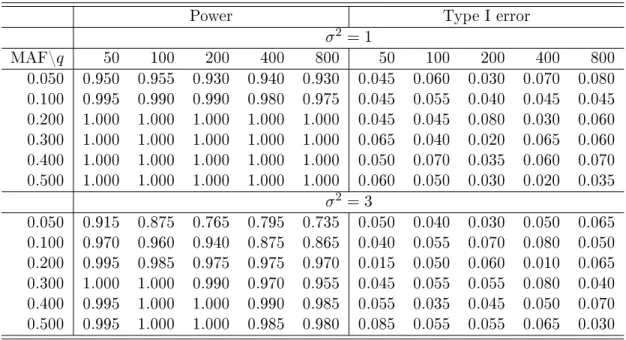
3.1 Simulation 1: power and type I error are reported for two sample test at 5 dierentqs at signicance
levelα= 5% whenσ2 = 1. . . 42 3.2 Simulation 1: power and type I error are reported
for two sample test at 5 dierentqs at signicance
levelα= 5% whenσ2 = 3. . . 43 3.3 Correlation matrix of responses used in the simulation . . . 43 3.4 Simulation 2: the estimates of rejection rates were
reported at 6 dierent MAFs, 5 dierent qs, and
2 dierent σ2 values at signicance level α = 5%.
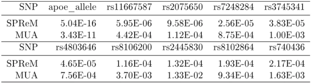
For each case, 100 simulated data sets were used. . . 43 3.5 Comparison between SPReM and the massive
uni-variate analysis (MUA) for ADNI data analysis: the top 10 SNPs and their −log10(p) values for
λ=λmax. . . 44
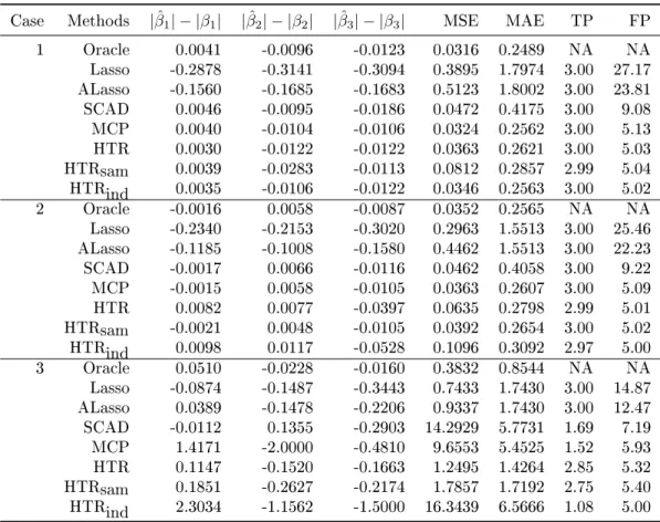
4.1 Mean of simulation results for p= 40: |βˆ1| − |β1|, |βˆ2| − |β2|,|βˆ3| − |β3|, MSE, MAE, TP, and FP. For
each case, 100 simulated data sets were used. . . 59 4.2 Median of simulation results forp= 40: |βˆ1| − |β1|,
|βˆ2| − |β2|,|βˆ3| − |β3|, MSE, MAE, TP, and FP. For
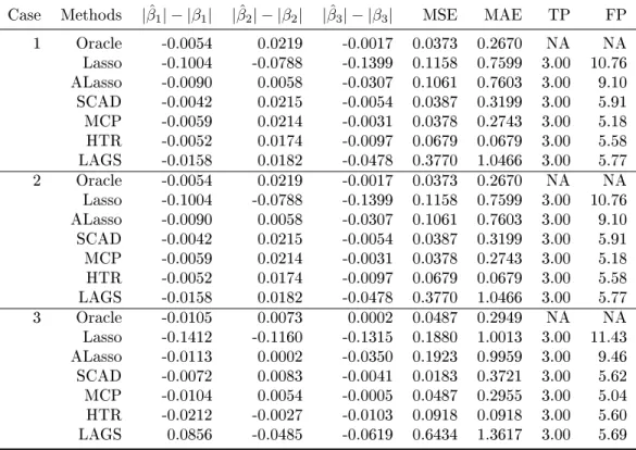
each case, 100 simulated data sets were used. . . 60 4.3 Mean of simulation results forp= 2000: we report
|βˆ1| − |β1|,|βˆ2| − |β2|,|βˆ3| − |β3|, MSE, MAE, TP,
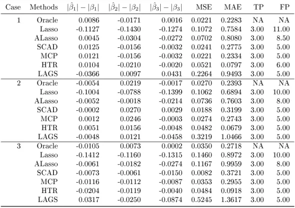
and FP. For each case, 100 simulated data sets were used. . . 61 4.4 Median of simulation results for p= 2000: we
re-port|βˆ1| − |β1|,|βˆ2| − |β2|,|βˆ3| − |β3|, MSE, MAE, TP, and FP. For each case , 100 simulated data
5.1 Setting 1: independent features setting. We report the Median Testing Classication Error (MTE) in percentage, the Median of number of nonzero co-ecients (denoted as s) and their standard
devia-tions (in parentheses). . . 88 5.2 Setting 2: Sparse Signal with Power Decay
Cor-relation. We report the Median Testing Classi-cation Error in percentage and its standard
devia-tions (in parentheses). . . 88 5.3 Setting 2:Sparse Signal with Power Decay
Correla-tion. We report the Median of number of nonzero coecients and its standard deviations (in
paren-theses). . . 88 5.4 Setting 3: Sparse Signal With Equal Correlation.
We report the Median Testing Classication Error
in percentage and its standard deviations (in parentheses). . . 89 5.5 Setting 3: Sparse Signal With Equal Correlation.
We report the Median of number of nonzero
coef-cients and its standard deviations (in parentheses). . . 89 5.6 Setting 4: Sparse Signal With Block Diagonal
Cor-relation. We report the Median Testing Classica-tion Error in percentage and its standard
devia-tions (in parentheses). . . 89 5.7 Setting 4: Sparse Signal With Block Diagonal
Cor-relation. We report the Median of number of nonzero coecients and its standard deviations (in
paren-theses). . . 90 5.8 Setting 5& 6: Sparse Signal with Sparse
Correla-tion or Sparse Precision Matrix. We report the Me-dian Testing Classication Error (MTCE) in per-centage, the Median of number of nonzero coe-cients in both projection directions (denoted ass1 and s2 respectively) and their standard deviations (in parentheses) in both of Sparse Correlation (SC)
setting and Sparse Precision (SP) setting. . . 90 5.9 Real data analysis: We report Median Test
Clas-sication Error (MTE) and Median of number of
LIST OF FIGURES
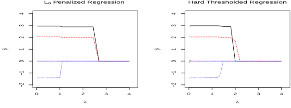
2.1 Solution paths ofL0 regularization regression and HTR: We consider a simple example that yi = xiβ+εi, where β = (3,2,−1.5,0,0,0)T and εi's
are independently and identically distributed as
N(0,1). We plot the estimates of regression co-ecients βˆj, j = 1,2, . . . ,6 for this example. Left Panel L0Penalized Regression estimates, as a func-tion of λ; Right Panel Hard Thresholded
Regres-sion estimates, as a function of λ. . . 11
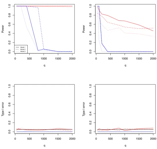
3.1 Simulation 1 results: the estimated rejection rates as functions of q for two dierent σ2 values. The
upper and lower rows are, respectively, for powers and for type I error rates, whereas the left and right columns correspond to σ2 = 1 and σ2 = 3, respectively. In all panels, the lines obtained from SPReM and RP are, respectively, presented in red and in blue, and the results for indepen-dence, weak, and strong correlation structures are, respectively, presented as thick, dashed, and
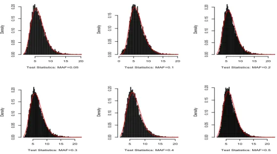
dot-ted lines. . . 39 3.2 Histograms and their gamma approximations based
on the wild bootstrap samples under the null
hy-pothesis for dierent MAFs forλ=λmax. . . 40
3.3 QQ-plot of the gamma approximations based on the wild bootstrap samples under the null
hypoth-esis for dierent MAFs forλ=λmax. . . 41
3.4 ADNI GWAS results: Manhattan plot of−log10(p)
CHAPTER1: INTRODUCTION
CHAPTER2: LITERATURE REVIEW
Traditionally, statistical inference considers a probability model for a population and con-siders data that arose as a sample from the population. For many problems, the estimates of the population characteristics, or parameters, can be substantially rened as the sample size n towards innity with xed number of unknown parameters p. Recently, researchers
are interested in high dimensional statistical inference, when the number of unknown pa-rameterspis much larger than the sample sizen, that ispn. This encompasses supervise
regression and classication models where the number of covariates is of much larger order thann, unsupervised settings such as clustering or graphical modeling with more variables
than observations or multiple testing where the number of considered testing hypotheses is larger than sample size. Such framework has become increasingly frequent and important in diverse elds of sciences, engineering, and humanities, ranging from genomics and health sciences to economics, nance and machine learning and characterizes many contemporary problems in statistics. For example, in imaging genetic studies between genotypes and phe-notypes, hundreds of thousands of as single-nucleotide polymorphisms (SNPs) are considered as potential covariates for high dimensional imaging measures; in disease classication using microarray or proteomics data, tens of thousands of expression s of molecules are potential predictors. When interactions are considered, the dimensionality grows exponentially and result in ultra-high dimensionality, where ultra-high dimensionality refers to the case where the dimensionality grows at a non-polynomial rate as the sample size increases. Donoho et al. (2000) convincingly demonstrates the need for developments in high dimensional data analysis and presents the curses and blessings of dimensionality.
and computational complexity, while in conventional studies, when the sample sizenis much
larger than the number of variables or parameters p, none of the three aspects needs to be
sacriced for the eciency of others. However, traditional method fails due challenges posed by high dimensionality. We introduce the diculties introduced by high dimensionality in the following.
A notorious diculty of high dimensional model selection comes from the collinearity among the predictors, as pointed out by Fan and Lv (2008). The collinearity can easily be spurious in high dimensional geometry, which can make us select a wrong model and thus lead to completely wrong scientic conclusions. Statistically, this is due to the model identiability issues in high dimensional framework.
Another well recognized issue for high dimensional statistical analysis goes to the noise accumulation problem both in statistics and computer science. The quantication of the impact of high dimensionality has been fully characterized both in regression and classica-tion problems (Bühlmann and Geer 2011). The predicclassica-tion error can be unbounded while the classication error can be as bad as random guessing due to noise accumulation in estimating the coecient parameters and the population centroids respectively.
The philosophy that will generally rescue us, is to "believe" that in fact only a few, says0 of the unknown parameters are non-zero, namely the parameters are assumed to be sparse. With sparsity, variable selection can improve estimation accuracy and model interpretability by eectively identifying the subset of important predictors and thus achieving parsimonious representation.
Sparsity arises in many scientic endeavors. In genomic studies, it is generally believed that only a fraction of molecules are related to biological outcomes. For example, in disease classication, it is commonly believed that only one specic gene or tens of genes are re-sponsible for the disease development. Selection tens of genes helps not only statisticians in constructing a more reliable classication rule, but also biologists to understand molecular mechanisms.
as pointed out in Fan and Li (2006), it is helpful to dierentiate two types of statistical endeavors in high dimensional statistical learning: accuracy of estimated model parameters by controlling the risk bound and accuracy of the expected loss of the estimated model. The former is called consistency and appears in many contexts where we want to identify the signicant predictors and characterize the precise contribution of each to the response variable. The latter property is called persistence in Greenshtein et al. (2004) and arises frequently in machine learning problems such as classication. More recently, Fan and Li (2001) has proposed the oracle property for high dimensional sparse regression by requiring the estimator identifying the true subset model and achieving the optimal estimation rate simultaneously.
Another important issue involves the estimation of a covariance matrix or its inverse (the precision matrix). Examples include portfolio management and risk assessment (Fan et al. 2008), high dimensional classication such as the Fisher discriminant (Hastie et al. 2009), graphic models (Meinshausen and Bühlmann 2006), statistical inference such as controlling false discoveries in multiple testing (Leek and Storey 2008, Efron 2010), nding quantitative trait loci based on longitudinal data (Yap et al. 2009, Xiong et al. 2011) and testing the capital asset pricing model (Sentana 2009), among others. Yet, the dimensionality is often either comparable with the sample size or even larger. In such cases, the sample covariance is known to have poor performance (Johnstone 2001), and some regularization is needed.
The major contribution of this dissertation involves building a framework of high di-mensional hypothesis test, a framework of simultaneous variable selection and estimation and a unied framework for sparse multicategory discriminant analysis. All of the projects involve incorporating covariance estimation into the regression framework to better trade o between noise accumulation and correlation modeling for possibility of relaxing conditions for consistent variable selection. We will separately introduce the the back ground in the following sections respectively.
2.0.1 Multivariate Regression and High Dimensional Test
Multivariate regression modeling with a multivariate responsey∈Rqand a multivariate covariate x ∈Rp is a standard statistical tool in modern high-dimensional inference, with wide applications in various large-scale applications, such as genome-wide association studies (GWAS) and neuroimaging studies. For instance, in GWAS, our primary problem of interest is to identify genetic variants (x) that cause phenotypic variation (y). Specically, in imaging genetics, multivariate imaging measures (y), such as volumes of regions of interest (ROIs), are phenotypic variables, whereas covariates (x) include single nucleotide polymorphisms (SNPs), age, and gender, among others. The joint analysis of imaging and genetic data may ultimately lead to discoveries of genes for neuropsychiatric and neurological disorders such as autism and schizophrenia (Scharinger et al. 2010, Paus 2010, Peper et al. 2007, Chiang et al. 2011). Moreover, in many neuroimaging studies, there is a great interest in the use of imaging measures (x), such as functional imaging data and cortical and subcortical structures, to predict multiple clinical and/or behavioral variables (y) (Knickmeyer et al. 2008, Lenroot and Giedd 2006). This motivates us to systematically investigate a multivariate linear model with a multivariate response y and a multivariate covariatex.
Throughout this paper, we considernindependent observations(yi,xi)and a
Multivari-ate Linear Model (MLM) given by
where Y = (y1, . . . ,yn)T, X = (x1, . . . ,xn)T, and B = (βjl) is a p×q coecient matrix
with rank(B) =r? ≤min(p, q). Moreover, the error termE= (e1, . . . ,en)T hasE(ei) = 0
and Cov(ei) = ΣR for all i, whereΣR is aq×q matrix. Many hypothesis testing problems
of interest, such as comparison across groups, can often be formulated as
H0:CB=B0 v.s. H1 :CB6=B0, (2.2)
whereCis anr×p matrix andB0 is anr×q matrix. Without loss of generality, we center
the covariates, standardize the responses, and assume rank(C) =r.
We focus on a specic setting that q is relatively large, butp is relatively small. Such a
setting is general enough to cover two-sample (or multi-sample) hypothesis testing for high-dimensional data (Chen and Qin 2010, Lopes et al. 2011). There are at least three major challenges including (i) a large number of regression parameters, (ii) a large covariance matrix, and (iii) correlations among multivariate responses. When the number of responses and the number of covariates are even moderately high, tting the conventional MLM usually requires estimating a p×q matrix of regression coecients, whose number pqcan be much
larger than n. Although accounting for complicated correlations among multiple responses
is important for improving the overall prediction accuracy of multivariate analysis (Breiman and Friedman 1997, Cook et al. 2010), it requires estimatingq(q+ 1)/2unknown parameters in an unstructured covariance matrix.
There is a great interest in the development of ecient methods for handling MLMs with large q. Four popular traditional methods include the mass univariate analysis, the
Hotelling's T2 test, partial least squares regression, and dimension reduction methods. As
pointed by Klei et al. (2008) and many others, testing each response variable individually in the mass univariate analysis requires a substantial penalty of controlling for multiplicity. The Hotelling'sT2 test is not well-dened, when q > n. Even when q≤n, the power of the
Hotelling's T2 can be very low if q is nearly as large as n. Partial least squares regression
(Chun and Keles 2010, Krishnan et al. 2011), but it focuses on prediction and classication. Although dimension reduction techniques, such as principal component analysis (PCA), are considered to reduce the dimensions of both the response and covariates (Formisano et al. 2008, Kherif et al. 2002, ROWE and Homann 2006, Teipel et al. 2007), most of the methods ignore the variation of covariates and their associations with responses. Thus, such methods can be sub-optimal for our problem.
Some recent developments primarily include regularization methods and envelope models (Peng et al. 2010, Tibshirani 1996, Breiman and Friedman 1997, Cook et al. 2010, Cook, R. D., Helland, I. S. and Su 2013, Lin et al. 2012). Cook, Li and Chiaromonte (2010) developed a powerful envelope modeling framework for MLMs. Such envelope methods use dimension reduction techniques to remove the immaterial information, while achieving ecient estimation of the regression coecients by accounting for correlations among the response variables. However, the existing envelope methods are limited to then >max(p, q) scenario. Recently, much attention has been given to regularization methods for enforcing sparsity inB(Peng et al. 2010, Tibshirani 1996). These regularization methods, however, do not provide a standard inference tool (e.g., standard deviation) on the regression coecient matrixB. Lin et al. (2012) developed a projection regression model (PRM) and its associated estimation procedure to assess the relationship between a multivariate phenotype and a set of covariates without providing any theoretical justication.
variables and covariates of interest, such as genetic markers. Simulations show that our method can control the overall Type I error well, while achieving high statistical power.
2.0.2 High Dimensional Sparse Regression Consider the linear model
yi =xTi β+εi, i= 1, . . . , n, (2.3)
wher yi is a univariate response, xi = (xi,1, . . . , xi,p)T is ap−dimensional covariate vector, β= (β1, . . . , βp)T is ap×1regression coecient vector, and{i :i= 1, . . . , n}are
indepen-dent and iindepen-dentically distributed (i.i.d) errors. The theory of linear models is well established for traditional applications, where the dimension p is xed and the sample size n is much
larger than p. With the development of many modern technologies, however, in many
bio-logical, medical, social, and economical studies, p is comparable with, or much larger than, n, making valid statistical inferences a great challenge. Let A be subset of indices such that A={j|βo
j 6= 0} and pA be the cardinality of A, where βo = (β1o, . . . , βpo)T is the true
parameter β. For prediction accuracy and variable selection consistency, it is common to
assume a sparsity assumption, that is, pA<< p.
For model (2.3), many regularization methods for variable selection minimize
Q(β) = 1
2n||y−Xβ||
2 2+
p X
j=1
pλ(βj), (2.4)
where y = (y1,· · · , yn)T, X is an n×p non-stochastic matrix with the ith row xTi, || · ||2 represents theL2norm, andpλ(·)is a penalty function (e.g., SCAD or Lasso), which depends
on a tuning parameter λ > 0. The most well-known best subset selection corresponding to the L0 penalty function can achieve simultaneous parameter estimation and variable selection (Akaike 1973, Schwarz 1978). The subset selection methods coupled with dierent selection criteria-including the Cp statistics, the Akaike information criterion (AIC), the
ination criterion (RIC) are special cases of the L0 penalized regression, resulting from the assignment of dierent values to λ. However, solving the L0 regularization with a xed λ is an NP-hard problem and its computational methods based on exhaustive search
rapidly become impractical when the number of covariates increases (Huo and Ni 2007, Fan and Peng 2004, Fan and Li 2001, Zhang 2010). To address such computational issue, dierent convex/nonconvex penalty functions have been used in Q(β) and been extensively investigated in order to mimic the L0 regularization (Tibshirani 1996, Fan and Li 2001, Fan and Peng 2004, Zhang 2010, Meinshausen and Bühlmann 2006, Leng et al. 2004, Zou 2006). Instead of developing another penalty function, we develop a new hard thresholded regression (HTR) modeling framework for performing simultaneous variable selection and unbiased estimation in model (2.3) in this dissertation. The key idea of HTR is to minimize
H(β) =||W×XT(y−Xβ)||1+λ||β||1, (2.5)
where W is a p0×p weighted matrix based on some initial estimates of β, which will be introduced in Section 2. As shown in Sections 2 and 3, HTR simultaneously enjoys two key computational and theoretical properties as follows.
(i) Since H(β) is convex and HTR can be casted as a linear program, minimizing
H(β) is computationally ecient even in high-dimensional settings.
(ii) Under some mild conditions, the HTR estimate, which minimizes H(β), is an oracle estimator and achieves unbiased estimation.
Due to its nice properties (i) and (ii), our HTR estimate may be a good addition to the extensive regularization literature.
Ip, whereIp is ap×pidentity matrix. A comparison of the regularization path between the L0 regularization regression and HTR is shown in Figure 2.1.
Our HTR diers signicantly from the regularization methods (2.5) in several major ways. A major advantage of HTR over nonconvex regularizations is its computational e-ciency (i), even though they may enjoy nice theoretical properties, such as oracle property (Barron et al. 1999, Lin et al. 2008). Although there are many impressive works on non-convex regularization methods (Wang et al. 2013a, Kim and Kwon 2012, Zhang and Zhang 2012, Fan and Lv 2011, Kim et al. 2008, Wang et al. 2013b), several important questions still remain. Specically, due to the non-convexity of the penalty function, multiple local minima always exist, while it is diculty to identify the oracle estimator among multiple minima, even if the oracle estimator may be known to exist along the solution path.
A major advantage of HTR over convex regularization methods is its nice theoretical property (ii). Due to the convexity of the penalty function, convex regularization methods, such as Lasso, suer from the bias issue and thus they can be suboptimal in terms of risk estimation. See Fan and Li (2001) for detailed discussions. Moreover, the shrinkage bias introduced by convex regularization methods poses major challenges to statistical inferences, such as constructing condence intervals or testing, in high dimensional settings (Zhang and Zhang 2011, van de Geer et al. 2013, Chatterjee and Lahiri 2011). There is a major conict of optimal prediction and consistent variable selection in the lasso method (Meinshausen and Bühlmann 2006, Leng et al. 2004, Zou 2006).
We make three major contributions in this part as follows.
We systematically investigate a fast two-step estimation procedure for HTR. The rst step is to calculate a ridge estimator and the second step is to solve a linear program-ming.
0 1 2 3 4
−2
−1
0
1
2
3
4
L0 Penalized Regression
λ
β
^
0 1 2 3 4
−2
−1
0
1
2
3
4
Hard Thresholded Regression
λ
β
^
Figure 2.1: Solution paths of L0 regularization regression and HTR: We consider a simple example that yi =xiβ+εi, where β= (3,2,−1.5,0,0,0)T and εi's are independently and
identically distributed as N(0,1). We plot the estimates of regression coecients βˆj, j =
1,2, . . . ,6 for this example. Left Panel L0 Penalized Regression estimates, as a function of
λ; Right Panel Hard Thresholded Regression estimates, as a function of λ.
We propose to incorporate the regularized covariance estimator into the estimation procedure in order to better trade o between noise accumulation and correlation modeling.
2.0.3 Sparse Multicategory Discriminant Analysis
When the feature space dimensionpis far more larger than the sample sizen, the Fisher's
linear discriminant rule fails owing to diverging spectra as demonstrated by Bickel and Levina (2008b), who showed that the independence rule in which the correlation structure is ignored performs better than the naive bayes rule. However, in my data analysis, for example, the microarray studies, correlation structure can is an essential characteristic of the data and is usually not negligible. To circumvent this issue, Fan et al. (2012) proposes the regularized optimal ane discriminant (ROAD) method. Their method focuses on the binary classication problem, where, on the other hand, many real world problems have more than two classes to deal with. Typical examples include text catergorization and microarray data analysis, etc. Witten and Tibshirani (2011) proposes the penalized LDA and extend the framework to multicategoty problem by using a sequential approach. However, their problem is not convex and is extremely computational expensive.
In this paper we propose a unied approach, called sparse multicategory discriminant analysis (SMDA), which enjoys following attractive properties.
It reduces to penalized version of the ROAD estimator when there are only two classes. It results a fast convex programming algorithm comparing to the penalized LDA
frame-work proposed by Witten and Tibshirani (2011).
CHAPTER3: SPARSE PROJECTION REGRESSION MODEL
We develop a Sparse Projection Regression Model (SPReM) framework to perform mul-tivariate regression modeling with a large number of responses and a mulmul-tivariate covariate of interest. We propose two novel heritability ratios to simultaneously perform dimension reduction, response selection, estimation, and testing, while explicitly accounting for cor-relations among multivariate responses. Our SPReM is devised to specically address the low statistical power issue of many standard statistical approaches, such as the Hotelling's
T2 test statistic or a mass univariate analysis, for high-dimensional data. We formulate
the estimation problem of SPReM as a novel sparse unit rank projection (SURP) problem and propose a fast optimization algorithm for SURP. Furthermore, we extend SURP to the sparse multi-rank projection (SMURP) by adopting a sequential SURP approximation. Theoretically, we have systematically investigated the convergence properties of SURP and the convergence rate of SURP estimates. Our simulation results and real data analysis have shown that SPReM outperforms other state-of-the-art methods.
3.1 Model Setup and Heritability Ratios
We introduce SPReM as follows. The key idea of our SPReM is to appropriately project yi in a high-dimensional space onto a low-dimensional space, while accounting for the
cor-relation structure ΣR among the response variables and the hypothesis test in (2.2). Let
W = [w1,· · · ,wk]be aq×knonrandom and unknown direction matrix, wherewj areq×1
vectors. A projection regression model (PRM) is given by
where βw is a p×k regression coecient matrix and the random vector εi hasE(εi) = 0
and Cov(εi) =WTΣRW. Whenk= 1, PRM reduces to the pseduo-trait model considered
in (Amos et al. 1990, Amos and Laing 1993, Klei et al. 2008, Ott and Rabinowitz 1999). If
k <<min(n, q)and W were known, then one could use likelihood (or estimating equation) based methods to eciently estimate βw, and (2.2) would reduce approximately to
H0W :Cβw=b0 v.s. H1W :Cβw6=b0, (3.2)
where Cβw=CBW andb0 =B0W. In this case, the number of null hypotheses in (3.2) is much smaller than that of (2.2). It is also expected that dierent W's strongly inuence the statistical power of testing the hypotheses in (2.2).
A fundamental question arises
“how do we determine an `optimal' W to achieve good statistical power of testing (2.2)?”
To determine W, we develop a novel deation approach to sequentially determine each column of W at a time starting from w1 to wk. We focus on how to determine w1 below and then discuss how to extend it to the scenario with k >1.
To determine an optimal w1, we consider two principles. The rst principle is to maximize the mean value of the square of the signal-to-noise ratio, called the heritabil-ity ratio, for model (3.1). For each i, the signal-to-noise ratio in model (3.1) is dened
as the ratio of mean to standard deviation of a signal or measurement wTyi, denoted by
SNRi=wTBTxi/(wTΣRw)0.5. Thus, the heritability ratio (HR) is given by
HR(w) =n−1 n X
i=1 SNR2
i =
wTBTSXBw wTΣ
Rw
, (3.3)
where SX = n−1Pni=1xixTi . The HR has several important interpretations. If thexi are
n→ ∞, we have
HR(w)→p w
TBTΣ XBw
wTΣ Rw
= Var(w
TBTx i)
Var(εi) ,
where →p denotes convergence in probability. Thus, HR(w) is close to the ratio of the
variance of signalwTBTx
i to that of noiseεi. Moreover, HR(w) is close to the heritability
ratio considered in (Amos et al. 1990, Amos and Laing 1993, Klei et al. 2008, Ott and Rabinowitz 1999) for familial studies, but we dene HR from a totally dierent perspective. With such new perspective, one can easily dene HR for more general designs, such as cross-sectional or longitudinal design. One might directly maximize HR(w) to calculate an `optimal' w1, but such a w1 can be sub-optimal for testing the hypotheses in (2.2) as discussed below.
The second principle is to explicitly account for the hypotheses in (2.2) under model (2.1) and the reduced ones in (3.2) under model (3.1). We dene four spaces associated with the null and alternative hypotheses of (2.2) and (3.2) as follows:
SH0 ={B:CB=B0}, SHW ={B:CBW=B0W}, SH1 ={B:CB6=B0}, SH1W ={B:CBW6=B0W}.
It can be shown that they satisfy the following relationship:
SH0 ⊂SHW and SH1W ⊂SH1 for anyW 6=0.
Due to potential information loss during dimension reduction, both SHW −SH0 and SH1 − SH1W may not be the empty set, but we need to chooseWsuch that SH1−SH1W ≈ ∅. The
next question is how to achieve this.
We consider a data transformation procedure. LetC1 be a(p−r)×pmatrix such that
Let D = [CT CT1]T be a p×p matrix and x˜i = (˜xTi1,x˜Ti2) = D−Txi be a p ×1 vector,
where x˜i1 and x˜i2 are, respectively, the r×1 and (p−r)×1 subvectors of x˜i. We dene
˜
B = [ ˜BT1 B˜T2]T = DBor B =D−1B˜, where B1˜ and B2˜ are, respectively, the rst r rows
and the last p−r rows of B˜. Therefore, model (3.1) can be rewritten as
WTyi = (D−1BW˜ )Txi+WTei (3.5)
= WT( ˜B1−B0)Tx˜i1+WTBT0x˜i1+WTB˜T2x˜i2+WTei.
In (3.5), due to (3.4), we only need to consider the transformed covariate vector x˜i1, which
contains useful information associated with B˜1−B0 =CB−B0.
We dene a generalized heritability ratio based on model (3.5). Specically, for eachi,
we dene a new signal-to-noise ratio as the ratio of mean to standard deviation of signal wT( ˜B1 −B0)Tx˜i1 +wTei, denoted by SNRi,C = wT( ˜B1 −B0)T˜xi1/(wTΣRw)0.5. The
generalized heritability ratio is then dened as
GHR(w;C) =n−1 n X
i=1 SNR2
i,C=
wT( ˜B1−B0)TSX1˜ ( ˜B1−B0)w wTΣ
Rw
, (3.6)
whereSX1˜ =n−1Pni=1x˜i1x˜Ti1. If thexis are random, then we have
GHR(w;C)→p w
T( ˜B1−B0)TCov(˜x
i1)( ˜B1−B0)w wTΣ
Rw
= w
TΣ Cw
wTΣ Rw
, (3.7)
where ΣC = ( ˜B1 −B0)T(D−TΣXD−1)(r,r)( ˜B1−B0), and (D−TΣXD−1)(r,r) is the upper
r×r submatrix of D−TΣXD−1. Particularly, if C= [Ir0], then ΣC reduces to wT( ˜B1− B0)T(ΣX)(1,1)( ˜B1 −B0)w, in which (ΣX)(1,1) is the upper r×r submatrix of ΣX. Thus,
GHR(w;C) can be interpreted as the ratio of the variance of wT( ˜B1−B0)Tx˜i1 relative to that of wTei. We propose to calculate an optimalw∗ as follows:
w∗ = argmax
w GHR
We expect that such an optimal w∗ can substantially reduce the size of both SH1 −SH1W
and SHW −SH0 and thus the use of such an optimal w∗ can enhance the power of testing
the hypotheses in (2.2). Without loss of generality, we assume B0 =0 from now on. We consider a simple example to illustrate the appealing properties of GHR(w;C).
Example We consider model (2.1) withp=q= 5and want to test the nonzero eect of the rst covariate on all ve responses. In this case, r= 1,C= (1,0,0,0,0),B0 = (0,0,0,0,0), and D=I5, which is a5×5identity matrix. Without loss of generality, it is assumed that (ΣX)(1,1)= 1.
We consider three dierent cases ofΣRandB. In the rst case, we setΣR=diag(σ12,· · · , σ52) and the rst column of B to be(1,0,0,0,0). It follows from (3.6) that
GHR(w;C) = w
2 1
σ21w12+σ22w22+· · ·+σ25w25 andw T
∗ = (c0,0,0,0,0),
wherec0 is any nonzero scalar. Therefore,w∗ picks out the rst response, which is the sole one that is associated with the rst covariate.
In the second case, we set ΣR=diag(σ21,· · ·, σ52) withσ21 ≥ · · · ≥σ25 and the rst row of B to be(1,1,0,0,0). It follows from (3.6) that
GHR(w;C) = (w1+w2) 2
σ21w21+σ22w22+· · ·+σ52w25 and w T
∗ = (
σ22
σ12c0, c0,0,0,0),
where c0 is any nonzero scalar. Therefore, w∗ picks out both the rst and second response with larger weight on the second component. This is desirable since β11 and β21 are equal in terms of strength of eect and the noise level for the second response is smaller than that of the rst one.
(3.6) that
GHR(w;C) = (w1+w2) 2
σ2w2
1+ 2σ22ρw1w2+σ22w22+Q(w3, w4, w5)
and w∗T = (c0, c0,0,0,0),
whereQ(w3, w4, w5)is a non-negative quadratic form of (w3, w4, w5). Thus, the optimalw∗ chooses the rst two responses with equal weight, since they are correlated with each other with same variance and β11=β21= 1.
For high dimensional data, it is dicult to accurately estimate w∗, since the sample covariance matrix estimatorΣˆRcan be either ill-conditioned or not invertible for largeq > n. One possible solution is to focus only on a small number of important features for testing. However, a naive search for the best subset is NP-hard. We develop a penalized procedure to address these two problems, while obtaining a relatively accurate estimate of w. Let Σ˜R
andΣˆC be, respectively, estimators ofΣRandΣC. Here we useΣ˜Rto denote the covariance estimator other than sample covariance matrix ΣˆR. To obtain ΣˆC, we need to plug Bb, an estimator of B, intoΣC. Without loss of generality, we consider the ordinary least squares
estimate of B. By imposing a sparse structure on w1, we recast the optimization problem as
max{w
TΣˆCw
wTΣ˜Rw} s.t.||w||1 ≤t, (3.9) where|| · ||1 is theL1 norm andt >0.
3.1.1 Sparse Unit Rank Projection
When`= (CB)T 6=0,(3.6)reduces to the following optimization problem:
w∗= argmax
wTΣRw=1
wTΣCw= argmax wTΣRw≤1
wTΣCw= argmax wTΣRw≤1
wT`, (3.10)
where ` is the sole eigenvector of ΣC, since ΣC is a unit-rank matrix. To impose an L1 sparsity on w, we propose to solve the penalized version of (3.10) given by
wλ = argmax wTΣRw≤1
wT`−λ||w||1. (3.11)
Although (3.11) can be solved by using some standard convex programming methods, such methods are too slow for most large-scale applications, such as imaging genetics. We there-fore reformulate our problem below. Without special saying, we focus on `= (CB)T 6=0. By omitting a scaling factor ||Σ−1R /2`||2, which will not aect the generalized heritability ratio, we note that (3.10)is equivalent to the following
w0= argmin
w
1 2w
TΣ
Rw−wT`. (3.12)
We consider a penalized version of (5.12) as
w0,λ= argmin w
f(w) = argmin
w
1 2w
TΣ
Rw−wT`+λ||w||1. (3.13)
A nice property of (5.13) is that it does not explicitly involve the inequality constraint, which leads to a fast computation. We dene(5.12)as the oracle, sincewλ converges tow0
asλ→0. It can be shown that
w0 = Σ−1R `. (3.14)
We obtain an equivalence between(5.13)and (3.11)as follows.
We discuss some connections between our SURP problem and the optimization prob-lem considered in Fan et al. (2012) for performing classication in high dimensional space. However, rather than recasting the problem as in (3.10) and then(5.13), they formulate it as
wc= argmin
||w||1≤c,wT`=1
wTΣRw,
which can further be reformulated as
wλ = argmin wT`=1
1 2w
TΣ
Rw+λ||w||1. (3.15)
Since (5.14) involves a linear equality constraint, they replace it by a quadratic penalty as
wλ,γ = argmin
1 2w
TΣ
Rw+λ||w||1+ 1 2γ(w
T`−1)2. (3.16)
This new formulation requires the simultaneously tuning of λand γ, which can be
compu-tationally intensive. However, in Fan et al. (2012), they stated that the solution to (5.15)is not sensitive toγ, since solution is always in the direction of Σ−1R `whenλ= 0, as validated by simulations. Their formulation (5.14) is close to the formulation(5.13). This result sheds some light on whywλ,γ is not sensitive toγ. Finally, we can show that the solution path to
(5.13) has a piecewise linear property.
Proposition 3.1.2 Let`∈Rq be a constant vector andΣR be positive denite. Then,w0,λ
is a continuous piecewise linear function in λ.
We derive a coordinate descent algorithm to solve (5.13). Without loss of generality, suppose that w = ( ˜w1,w˜2T)T = ( ˜w1,· · · ,w˜q)T, w˜j for all j ≥2 are given, and we need to
optimize (5.13) with respect to w˜1. In this case, the objective function (5.13) becomes
f1( ˜w1,w2˜ ) = 1 2( ˜w1,w˜
T
2)
σ11 Σ12 Σ21 Σ22
˜ w1 ˜ w2
−(˜`1w˜1+ ˜` T
where ` = (˜`1,`˜T2) and σ11,Σ12, and Σ22 are subcomponents of ΣR. Then, by taking the
sub-gradient with respect to w˜1, we have
f10( ˜w1,w˜2) = ˜w1σ11+ Σ12w˜2+λΓ1−`˜1
whereΓ1=sign( ˜w1)forw˜16= 0and is between−1and1ifw˜1 = 0. LetSλ(t) =sign(t)(|t| − λ)+ be the soft-thresholding operator. By setting f10( ˜w1,w2˜ ) = 0, we have w˜1 = Sλ(˜`1 − Σ12w2˜ )/σ11.Based on this result, we can obtain a coordinate descent algorithm as follows. Algorithm
(a) Initialize wat a starting point w(0) and setm= 0. (b) Repeat:
(b.1) Increasem by1: m←m+ 1
(b.2) forj∈1,· · · , p, if w˜j(m−1) = 0, then set w˜j(m)=0; otherwise: w˜(jm) = argminf( ˜w(1m),· · · ,w˜(jm−1),w˜j,w˜(m
−1)
j+1 ,· · ·,w˜ (m−1)
q )
(c) Until numerical convergence: we require|f(w(m))−f(w(m−1))|to be suciently small.
3.1.2 Extension to Multi-rank Cases
In this subsection, we extend the sparse unit rank projection procedure to handle multiple rank test problems when r >1. We propose the k−th projection direction as the solution to the following problem:
argmaxw
T kΣCwk
wT kΣRwk
s.t.wTkΣRwj = 0, ∀j < k. (3.17)
It can be shown that (3.17) is equivalent to
Following the reasoning in Witten and Tibshirani (2011), we recast(3.18)into an equivalent problem.
Proposition 3.1.3 Problem (3.18)is equivalent to the following problem:
argmax
w
wTBTCTΣ111/2P⊥k−1Σ111/2CBw wTΣ
Rw
, (3.19)
where P⊥k−1 is the projection matrix onto the orthogonal space spanned by{Σ111/2CBwj,1≤ j ≤k−1}, in which Σ11= (D−TΣXD−1)(r,r).
Based on Proposition3.1.3, we consider several strategies of imposing the sparsity struc-ture onwk. A simple strategy is to consider the following problem given by
argmax
wk
wTkΣkCwk−λ||wk||1 s.t. wTkΣRwk ≤1, (3.20)
where ΣkC =BTCTΣ111/2P⊥k−1Σ111/2CB. When the rank of C is greater than 1, the problem in (3.20) is no longer convex, since it involves maximizing an objective function that is not concave. A potential solution is to use the minorization-maximization (MM) algorithm (Lange et al. 2000). Specically, for any xed w(m), we take a Taylor series expansion of wTkΣkCwk at w(m) and get
wkTΣkCwk−λ||wk||1 ≥2wTkΣkCw
(m)
k −w
(m)T
k Σ
k Cw
(m)
k −λ||wk||1. (3.21)
Thus, the right hand side of (3.21) minorizes the objective function (3.20) at w(km) and is a convex function, which can be solved by using some convex optimization methods. However, based on our extensive experience, the MM algorithm is too slow for most large-scale problems, such as imaging genetics.
of (D−TΣXD−1)(r×r) as (D−TΣXD−1)(r×r) = Prj=1γj`j`Tj, where (γj,`j) are
eigenvalue-eigenvector pairs with γ1 ≥ γ2 ≥ · · · ≥ γr. Then, instead of solving (3.20), we propose to
solve r SURP problems as
wkλ= argmin1 2w
T
kΣRwk−
√
γk`TkCBwk+λk||wk||1 for 1≤k≤r. (3.22)
Solving (3.22) leads tor sparse projection directions. In (3.22), since we sequentially extract
the direction vector according to the input signal ΣC, it may produce a less informative
direction vector compared with those from (3.20). However, such formulation leads to a fast computational algorithm and our simulation results demonstrate its reasonable performance. Thus, (3.22) is preferred in practice.
3.1.3 Test Procedure
We consider three statistics for testingH0W againstH1W in (3.2). Based on model (3.1),
we calculate the ordinary least squares estimate ofβw, given byβˆw= (PNi=1xixTi )−1 PN
i=1xiyTi W.
Subsequently, we calculate a k×kmatrix, denoted by Tn, as follows:
Tn= (Cβˆw−b0)TΣ−1˜
Ω (Cβˆw−b0), (3.23) where ΣΩ˜ is a consistent estimate of the covariance matrix of Cβˆw−b0. Specically, let
˜
βw be the restricted least squares (RLS) estimate ofβ underH0, which is given by
˜
βw= ˆβw−(XTX)−1CT[C(XTX)−1CT]−1(Cβˆw−b0).
Then, we can set ΣΩ˜ = C(XTX)−1PNi=1a2ixi˜iT˜ixTi(XTX)−1CT, where ai = 1/{1 −
xTi (XTX)−1xi} and ˜i = WTyi −β˜ T
wxi. When k > 1, we use the determinant, trace
and eigenvalues of Tn as test statistics, which are given by
where det, trace, and eig, respectively, denote the determinant, trace and eigenvalues of a symmetric matrix. When k = 1, all three statistics in (3.24) reduce to the Wald-type (or Hotelling'sT2) test statistic. For simplicity, we focus on Trn throughout the paper.
We propose a wild bootstrap method to improve the nite sample performance of the test statistic Trn. First, we t model(2.1)under the null hypothesis (2.2)to calculate the
estimated regression coecient matrix, denoted by Bb0, with corresponding residuals ˆei =
yi−BbT0xi for i= 1, . . . , n. Then we generate Gbootstrap samplesz
(g)
i = (Bb0)Txi+η
(g)
i eˆi
for i= 1, . . . , n, where η(ig) are independently and identically distributed as a distribution F, which is chosen to be ±1 with equal probability. For each generated wild-bootstrap sample, we repeat the estimation procedure for estimating the optimal weights and the calculation of the test statistic Tr(g)
n . Subsequently, the p-value of Trn is computed as
1
G PG
g=11(Tr (g)
n ≥Trn), where1(·) is an indicator function.
3.1.4 Tuning Parameter Selection
We consider several methods to select the tuning parameter λ. The rst one is cross
validation (CV), which is primarily a way of measuring the predictive performance of a statistical model. However, the CV technique can be computationally expensive for large-scale problems. The second one is the information criterion, which has been widely to measure the relative goodness of t of a statistical model. However, neither of these two methods are applicable for SURP, since our primary interest is to nd informative directions for appropriately testing the null and alternative hypotheses of (2.2). If the null hypothesis is true, it is expected thatCBb only contains noisy components and the estimated direction
vectors should be random. In this case, the test statistics Trn,Wn, and Royn should not be
sensitive to the value of λ. This motivates us to use the rejection rate to select the tuning
parameter as follows:
ˆ
λ= argmax 0≤λ≤λmax
{(Rejection Rate)λ}, (3.25)
3.2 Asymptotic Theory
We investigate several theoretical properties of SURP and its associated estimator. By substituting Σ˜R and`b=CBb into (5.13), we can calculate an estimate of w0 as
ˆ
wλ= argmin w
1 2w
TΣ˜
Rw−wT`b+λ||w||1. (3.26)
The following question arises naturally: how close is wˆλ to w0?
We address this question in Theorems 3.2.1 and 3.2.2.
We consider the scenario that there are a few nonzero components in w0, that is, a few response variables are associated with the covariates of interest. Such a scenario is common in many large-scale problems. We make a note here that the sparsity ofw0 = Σ−1R ` does not require neither Σ−1R nor ` to be sparse, and hence are more quite exible. Let S0 = {j : w0,j 6= 0} be the active set of w0 = (w0,1,· · ·, w0,q)T and s0 is the number of elements in S0. We use the banded covariance estimator of ΣR (Bickel and Levina 2008b)
such that||Σ˜R−ΣR||2=Op((lognq)
α
2(α+1))for some well behaved covariance classU(ε
0, α, C1), which is dened as
U(ε0, α, C1) = {Σ = (σjj0) : max
j X
j0
{|σj0j|:|j0−j|> k} ≤C1k−α for allk >0
and 0< ε0≤λmin(Σ)≤λmax(Σ)≤1/ε0}.
We have the following results.
Theorem 3.2.1 Assume that ΣR∈ U(ε0, α, C1) and
λ= max{(knt01+C1kn−α)||w0||2, t02} (
log(q∨n)
n )
α
2(α+1)||w0||
2, (3.27)
wherekn(log(nq∨n))−
1 2(α+1),t0
1 :=
q
2(η1+ 1)γ(01,δ)
q
log(q∨n)
n , andt
0 2:= C0ε0
p
2(η2+ 1)
q
log(q∨n)
n)−η1−(q∨n)−η2, we have
||wˆλ−w0||2≤Cλ √
s0, (3.28)
where C is a constant not depending on q and n. Furthermore, for ||`||2> δ0, we have
|| wˆλ ||wˆλ||2
− w0 ||w0||2||2≤
2Cλ√s0
||w0||2 . (3.29)
Theorem3.2.1gives an oracle inequality and theL2 convergence rate ofwˆλ in the sparse
case, which indicates direction consistency and is important to ensure the good performance of test statistics. This result has several important implications. If √s0(lognq)
α
2(α+1) =o(1),
then ||wˆλ −w0||2 converges to zero in probability. Therefore, our SURP should perform well for the extremely sparse cases with s0 << n. This is extremely important in practice, since the extremely sparse cases are common for many large-scale problems. Although we consider the banded covariance estimator ofΣRin Theorem 3.2.1 (Bickel and Levina 2008b),
the convergence rate ofwˆλ can be established for other estimators ofΣR and `as follows.
Theorem 3.2.2 Suppose that we have ||Σ˜R−ΣR||2 = Op(an) = op(1) and ||`ˆ−`||∞ =
Op(bn) =op(1), then
||wˆλ−w0||2=Op((an∨bn)
√
s0). (3.30)
Furthermore, for ||`||2 > δ0, we have
|| wˆλ ||wˆλ||2
− w0 ||w0||2
||2 =Op(
(an∨bn)√s0 ||w0||2
). (3.31)
Theorem3.2.2gives theL2 convergence rate ofwˆλ for any possible estimators ofΣRand `. A direct implication is that we can consider other estimators of ΣR in order to achieve
better estimation of ΣR under dierent assumptions of ΣR. For instance, if ΣR has an
approximate factor structure with sparsity, then we may consider the principal orthogonal complement thresholding (POET) method in Fan et al. (2013) to estimate ΣR. Moreover,
scenario with large p. We will systematically investigate these generalizations in our future
work.
Remark The SPReM estimator wˆλ is closely connected with those estimators in Witten
and Tibshirani (2011) and Fan et al. (2012) in the framework of penalized linear discriminant analysis. However, little is known about the theoretical properties of such estimators. To the best of our knowledge, Theorems 3.2.1and 3.2.2are the rst results on the convergence rate of such estimators under the restricted eigen-vectors of problem (3.9).
Remark The SPReM estimatorwˆλdoes not have the oracle property due to the asymptotic
bias introduced by the L1 penalty. See detailed discussions in (Fan and Li 2001, Zou 2006). However, our estimation procedure may be modied to achieve the oracle property by using some non-concave penalties or adaptive weights. We will investigate this issue in more depth in our future work.
3.3 Numerical Examples
3.3.1 Simulation 1: Two Sample Test in High Dimensions
In this subsection, we consider high-dimensional two-sample test problems and compare SPReM with the High-dimensional Two-Sample test (HTS) method in Chen and Qin (2010) and the Random Projection (RP) method proposed by Lopes et al. (2011). Both HTS and RP are the state-of-the-art methods for detecting a shift between the means of two high-dimensional normal distributions. It has been shown in Lopes et al. (2011) that the random projection method outperforms several competing methods when q/nconverges to
a constant or∞.
We simulated two sets of samples{y1, ...,yn1}and{yn1+1, . . . ,yn}fromN(β1,ΣR)and N(β2,ΣR), respectively, where β1 and β2 are q ×1 mean vectors and ΣR = σ2(ρjj0), in
which (ρjj0) is a q ×q correlation matrix. We set n = 2n1 = 100 and the dimension of
problem can be formulated as a special case of model (2.1) withn=n1+n2. Moreover, we have BT = [β1,β2] and C = (1,−1). Without loss of generality, we set β1 = β2 = 0 to assess type I error rate and then introduce a shift in the rst ten components of β2 to be 1
to assess power. We set σ2 to be 1 and 3 and consider three dierent correlation matrices
as follows.
Case1 is an independent covariance matrix with (ρjj0) =diag(1,· · ·,1).
Case2 is a weak correlation matrix with ρjj0 =1(j0 =j) + 0.3×1(j0 6=j).
Case3 is a strong correlation covariance matrix with ρjj0 = 0.8|j 0−j|
.
Simulation results are summarized in Tables3.1and3.2. As expected, both HTS and RP perform worse asq gets larger, whereas our SPReM works very well even for relatively large q. This is consistent with our theoretical results in Theorems 3.2.1 and 3.2.2. Moreover,
HTS and RP cannot control the type I error rate well in all scenarios, whereas our SPReM based on the wild bootstrap method works reasonably well. According to the best of our knowledge, none of the existing methods for the two sample test in high dimensions work well in this sparse setting. For cases (ii) and (iii), Σ−1R (β1−β2) is not sparse, but SPReM performs reasonably well under the correlated scenarios. This may indicate the potential of extending SPReM and its associated theory to non-sparse cases. As expected, increasing
σ2 decreases statistical power in rejecting the null hypothesis. Since both SPReM and
RP signicantly outperform HTS, we increased q to 2,000 and presented some additional
comparisons between SPReM and RP based on 100 simulated data sets in Figure 1.
3.3.2 Simulation 2: Multiple Rank Cases
200, 400 and 800, respectively, and then simulated the multivariate phenotype according to model (1). The random errors were simulated from a multivariate normal distribution with mean0and covariance matrix with diagonal elements1. For the o-diagonal elements in the covariance matrix, which characterize the correlations among the multivariate phenotypes, we categorized each component of the multivariate phenotype into three categories: high correlation, medium correlation and very low correlation with the corresponding number of components (1,1, q−2)in each category, and then we set the three degrees of correlation among the dierent components of the multivariate phenotype according to Table 3. The nal covariance matrix is set to beΣR=σ2(ρjj0), where(ρjj0)is the correlation matrix. We
considered σ2 = 1 and3.
For the covariates, we included two SNPs with an additive eect and 3 additional con-tinuous covariates. We varied the minor allele frequency (MAF) of the rst SNP, whereas we xed the MAF of the second SNP to be 0.5. For the rst SNP, we considered 6 scenarios assuming the MAFs are 0.05, 0.1, 0.2, 0.3, 0.4, and 0.5, respectively. We simulated the three additional continuous covariates from a multivariate normal distribution with mean 0, standard deviation 1, and equal correlation 0.3. We rst set B= 0 to assess type I error rate. To assess power, we set the rst response to be the only components of the multivari-ate phenotype associmultivari-ated with the rst SNP and the second response to be the component related to the second SNP eect. Specically, we set the coecients of the two SNPs to be 1 for the selected responses and all other regression coecients to be 0. We are interested in testing the joint eects of the two SNPs on phenotypic variance.
We applied SPReM to 100 simulated data sets. Note that to the best of our knowledge, no other methods can be used to test the multi-rank test problem and thus we only focus on SPReM here. Table 4 presents the estimated rejection rates corresponding to dierent MAFs, q, andσ2. Our SPReM works very well even for relatively largeq under bothσ2 = 1 and 3. Specically, the wild bootstrap method can control the type I error rate well in all scenarios. For the power, SPReM performs reasonably well under the small MAFs and
size gets larger. As expected, increasing σ2 decreases statistical power in rejecting the null
hypothesis.
3.3.3 Alzheimer's Disease Neuroimaging Initiative (ADNI) Data Analysis The development of SPReM is motivated by the joint analysis of imaging, genetic, and clinical variables in the ADNI study. Data used in the preparation of this arti-cle were obtained from the Alzheimer's Disease Neuroimaging Initiative (ADNI) database (adni.loni.ucla.edu). The ADNI was launched in 2003 by the National Institute on Aging (NIA), the National Institute of Biomedical Imaging and Bioengineering (NIBIB), the Food and Drug Administration (FDA), private pharmaceutical companies and non-prot orga-nizations, as a $60 million, 5-year publicprivate partnership. The primary goal of ADNI has been to test whether serial magnetic resonance imaging (MRI), positron emission to-mography (PET), other biological markers, and clinical and neuropsychological assessment can be combined to measure the progression of mild cognitive impairment (MCI) and early Alzheimer's disease (AD). Determination of sensitive and specic markers of very early AD progression is intended to aid researchers and clinicians to develop new treatments and mon-itor their eectiveness, as well as lessen the time and cost of clinical trials. The Principal Investigator of this initiative is Michael W. Weiner, MD, VA Medical Center and University of California, San Francisco. ADNI is the result of eorts of many coinvestigators from a broad range of academic institutions and private corporations, and subjects have been recruited from over 50 sites across the U.S. and Canada. The initial goal of ADNI was to recruit 800 subjects but ADNI has been followed by ADNI-GO and ADNI-2. To date these three protocols have recruited over 1500 adults, ages 55 to 90, to participate in the research, consisting of cognitively normal older individuals, people with early or late MCI, and people with early AD. The follow up duration of each group is specied in the protocols for ADNI-1, ADNI-2 and ADNI-GO. Subjects originally recruited for ADNI-1 and ADNI-GO had the option to be followed in ADNI-2. For up-to-date information, see www.adni-info.org. "
818 subjects in the ADNI-1 database, which resulted in a set of 620,901 SNPs and copy number variation (CNV) markers. Since the Apolipoprotein E (ApoE) SNPs, rs429358 and rs7412, are not on the Human 610-Quad Bead-Chip, they were genotyped separately and added to the data set manually. For simplicity, we only considered the 10,479 SNPs collected on the chromosome19, which houses the famous ApoE gene commonly suspected of having association with Alzheimer's disease. A complete GWAS of ADNI will be reported elsewhere. The SNP data were preprocessed by standard quality control steps including dropping any SNP that has more than 5% missing data, imputing the missing values in each SNP with its mode, dropping SNPs with minor allele frequency <0.05, and screening out SNPs violating the Hardy-Weinberg equilibrium. Finally, we obtained 8,983SNPs on chromosome 19, including the ApoE allele as the last SNP in our dataset.
Our problem of interest is to perform a genome-wide search for establishing the asso-ciation between the 10,479 SNPs collected on the chromosome 19 and the brain volume of 93 regions of interest (ROIs). We tted model (1) with all 93 ROIs as responses and a covariate vector including an intercept, a specic SNP, age, gender, whole brain volume, and the top 5 principal components to account for population stratication. To reduce popula-tion straticapopula-tion eects, we only used 761 Caucasians from all 818 subjects. Subjects with missing values were removed, which leads to 747 subjects. We set λ=λmax in our SPReM for computational eciency. To test the SNP eect on all 93 ROIs, we calculated the test statistic and itsp−value for each SNP. We further performed a standard massive univariate analysis. Specically, we tted a linear model with the same set of covariates and calculated a p−value for every pair of ROIs and SNPs.
samples for each MAF group, we use the Satterthwaite method to approximate the null distribution of the test statistic by a Gamma distribution with parameters(aT, bT).
Speci-cally, we setaT =E2/V andbT =V/E by matching the mean (E) and the variance (V) of the test statistics and those of the Gamma distribution. The histograms and the tted gamma distributions along with the QQ-plots are, respectively, presented in Figures 2-3. Figures 2 and 3 reveal that our gamma approximations work reasonably well for a wide range of MAFs whenλ=λmax. Since we only use Gamma(aT, bT)to approximate thep−value of large test
statistic, we only need a good approximation at the tail of the Gamma distribution. See Figure 3 for details. For each SNP, we matched its MAF with the closest MAF group in the pool and then calculated the p−value of the test statistic based on the approximated gamma distribution. We present the manhattan plot in Figure 4 and the top 10 SNPs with their p−values for SPReM and the mass univariate analysis in Table 5 for λ=λmax.
3.4 Discussion
In this paper, we have developed a general SPReM framework based on the two heritabil-ity ratios. Our SPReM methodology has a wide range of applications, including sparse linear discriminant analysis, two sample tests, and general hypothesis tests in MLMs, among many others. We have systematically investigated theL2 convergence rate ofwˆλ in the ultra-high
dimensional framework. We further extend the SURP problem to the SMURP and oered a sequential SURP approximation algorithm. We carried out simulation studies and examined a real data set to demonstrate the excellent performance of our SPReM framework compared to other state-of-the-art methods.
3.5 Assumptions and Proofs
Throughout the paper, the following assumptions are needed to facilitate the technical details, although they may not be the weakest conditions.
Assumption A1. C(n−1XTX)−1CT 1, that is, there exists constant c0 and C0 such that c0≤C(n−1XTX)−1CT ≤C0.
Assumption A2. 0≤ε0≤λmin(ΣR)≤λmax(ΣR)≤1/ε0.
Assumption A3. The covariance estimatorΣ˜Rsatises: ||Σ˜R−ΣR||2=Op(an)≤op(1).
Remark : Assumption A1 is a very weak and standard assumption for regression models. Assumption A2 has been widely used in the literature. Assumption A3 requires a relatively accurate covariance estimator in terms of spectral norm convergence. We may use some good penalized estimators ofΣRunder dierent assumptions ofΣR(Bickel and Levina 2008b, Cai
et al. 2010, Lam and Fan 2009, Rothman et al. 2009, Fan et al. 2013).
Proof of Theorem 3.1.1 The Karush Kuhn Tucker (KKT) conditions for problem (3.11) are given by:
`−λΓ−γΣRw= 0, γ≥0, γ(
1 2w
TΣ Rw−
1 2) = 0,
1 2w
TΣ Rw≤
whereΓis aq×1vector and equals the subgradient of||w||1with respect tow. We consider two scenarios. First, suppose that |`j| > λ for some j. We must have γΣRw 6= 0, which
leads to γ >0 and wTΣRw= 1. Thus, the KKT conditions reduce to
`−λΓ−γΣRw= 0, γ ≥0, wTΣRw= 1.
If we write w˜ = γw, this is equivalent to solving problem (5.13) with w˜ and then take normalization. Second, if |`j| ≤λfor any j, thenw= 0and γ = 0, which is the solution of (5.13) as well. This nishes the proof.
Proof of Proposition 3.1.2 It follows from Theorem2 of Rosset and Zhu (2007).
Proof of Proposition 3.1.3 The proof is similar to that of Proposition 1 of Witten and Tibshirani (2011). Letting w˜k= Σ1R/2wk, then problem (3.18)can be rewritten as
argmaxw˜TkΣR−1/2BTCTΣ111/2CBΣ−1R /2w˜k s.t. ||w˜k||2≤1,
which is equivalent to
argmaxw˜kAP⊥k−1uk s.t ||w˜k||2 ≤1,||uk||2≤1, (3.32)
where A = BTCTΣ1/2
11 . Thus, w˜k and uk that solve problem (3.32) are the k-th left
and right singular vectors of A (Witten and Tibshirani 2011). Therefore, we have P⊥k−1 = I−Pkj=1−1ujuTj andukis thek-th eigenvector ofATA, or equivalently thek-th right singular
vector of A. For problem (3.32), w˜k is the k-th left singular vector of A. Therefore, the
solution of (3.19) is the k-th discriminant vector of (3.18).
Proof of Theorem 3.2.1 In this theorem, we specically use the banded covariance esti-mator Σ˜R=Bk
n( ˆΣR), whereBk(Σ) = [σjj0I(|j
0−j| ≤k)]andΣˆ
R is the sample covariance
matrix of yi−BˆTxi.
First, we deneJ ={||Σ˜R−Bkn(ΣR)||∞≤t1} T
specied as in Lemma 3.5.2. Then, it follows from Lemma 3.5.2 that P(J) ≥ 1−3(q∨
n)−η1−2(q∨n)−η2.
On the setJ, by taking λ= max{knt1+C1kn−α, t2} and using Lemma3.5.1, we have
1
2(wˆλ−w0)
TΣ˜
R(wˆλ−w0) +λ||wˆλ||1 ≤(wT0(ΣR−Σ˜R) +εT)(wˆλ−w0) +λ||w0||1 ≤ ||Σ˜R−ΣR||2||w0||2||wˆλ−w0||1+||ε||∞||wˆλ−w0||1+λ||w0||1
≤(knt1+C1kn−α)||w0||2||wˆλ−w0||1+t2||wˆλ−w0||1+λ||w0||1 ≤λ||wˆλ−w0||1+λ||w0||1.
Let w0,S0 = [w0,jI(j ∈S0)], wherew0,j is the j−th component ofw0. The above equation
can be rewritten as
(wˆλ−w0)T( ˜ΣR−ΣR+ ΣR)(wˆλ−w0) +λ||wˆλ,S0||1+λ||wˆλ,Sc 0||1
≤λ||wˆλ,S0 −w0,S0||1+λ||w0,S0||1+λ||wˆλ,Sc 0||1,
which yields
{λmin−O(1)( log(q)
n )
α 2(α+1)}||wˆ
λ−w0||22≤2λ √
s0||wˆλ−w0||2.
Finally, we obtain the following inequality
||wˆλ−w0||2 ≤
2λ√s0
λmin−O(1)(log(nq))2(αα+1)
≤Cλ√s0,
which nishes the proof.
Proof of Theorem 3.2.2 It follows from Lemma (3.5.1)that
1
2(wˆλ−w0)
TΣ˜