TCP RAPID: FROM THEORY TO PRACTICE
Qianwen Yin
A dissertation submitted to the faculty of the University of North Carolina at Chapel Hill in partial fulfillment of the requirements for the degree of Doctor of Philosophy in the Department of Computer Science.
Chapel Hill 2017
Approved by: Jasleen Kaur F. Donelson Smith Kevin Jeffay Jay Aikat
ABSTRACT
QIANWEN YIN: TCP RAPID : From Theory to Practice (Under the direction of Jasleen Kaur)
Delay and bandwidth-based alternatives to TCP congestion-control have been around for nearly three decades and have seen a recent surge in interest. However, such designs have faced significant resistance in being deployed on a wide-scale across the Internet—this has been mostly due to serious concerns about noise in delay measurements, pacing inter-packet gaps, and required changes to the standard TCP stack. With the advent of high-speed networking, some of these concerns become even more significant.
This thesis considers Rapid, a recent proposal for ultra-high speed congestion control, which perhaps stretches each of these challenges to the greatest extent. Rapid adopts a framework of continuous fine-scale bandwidth probing and rate adapting. It requires finely-controlled inter-packet gaps, high-precision timestamping of received packets, and reliance on fine-scale changes in inter-packet gaps. While simulation-based evaluations of Rapid show that it has outstanding performance gains along several important dimensions, these will not translate to the real-world unless the above challenges are addressed.
ACKNOWLEDGEMENTS
TABLE OF CONTENTS
LIST OF TABLES . . . xii
LIST OF FIGURES . . . xiii
LIST OF ABBREVIATIONS . . . xvi
1 Introduction . . . 1
1.1 Motivation . . . 1
1.1.1 Issues with Loss-based TCP Congestion Control . . . 1
1.1.2 Promises of Delay-based and Bandwidth-based Protocols . . . 2
1.1.3 Hurdles to Widespread Adoption . . . 3
1.1.4 RAPID Stretches Challenges to Extreme . . . 5
1.1.4.1 TCP RAPID —a Packet-scale Congestion Control Protocol . . . 5
1.1.4.2 Challenges in Practice . . . 6
1.1.5 Goal of this dissertation . . . 7
1.2 Challenges of RAPID in Practice . . . 7
1.2.1 Creating Accurate Inter-packet Gaps . . . 7
1.2.1.1 RAPID Requirement . . . 7
1.2.1.2 Challenges . . . 8
1.2.1.3 Goal . . . 8
1.2.2 Noise Removal to Achieve Accurate ABest . . . 8
1.2.2.1 RAPID Requirement . . . 8
1.2.2.2 Challenges . . . 9
1.2.2.3 Goal . . . 11
1.2.3 Stability/Adaptability Trade-off . . . 11
1.2.3.2 Challenges . . . 12
1.2.3.3 Goal . . . 12
1.2.4 Deployability Within TCP Stack . . . 12
1.2.4.1 RAPID Requirement . . . 12
1.2.4.2 Challenges . . . 13
1.2.4.3 “gap-clocking” vs “ack-clocking” . . . 13
1.2.4.4 Fine-scale Arrival Timestamping . . . 14
1.2.4.5 Goals . . . 14
1.3 Thesis Statement . . . 15
1.4 Contributions . . . 15
1.4.1 Creating Accurate IPGs . . . 15
1.4.2 Denoising for Accurate Bandwidth Estimation . . . 15
1.4.3 Addressing the Stability/Adaptability Trade-off . . . 16
1.4.4 Implementing on Standard Protocol Stacks. . . 16
1.4.4.1 Realizing gap-clocking . . . 16
1.4.4.2 Achieving Fine-scale Arrival Timestamping . . . 16
1.4.5 Evaluation of RAPID in Ultra-high-speed Testbed . . . 16
1.4.6 Apply the Lesson to Other Delay- and Rate-based Protocols . . . 17
1.5 Outline . . . 17
2 Background . . . 19
2.1 Historical Perspective of TCP Congestion Control . . . 19
2.1.1 Transport Control Protocol . . . 19
2.1.2 Loss-based Congestion Control . . . 20
2.1.2.1 NewReno . . . 21
2.1.2.2 BIC . . . 21
2.1.2.3 Cubic . . . 22
2.1.2.4 HighSpeed . . . 22
2.1.2.6 Hybla . . . 23
2.1.3 Delay-based and Rate-based Congestion Control . . . 23
2.1.3.1 Vegas . . . 24
2.1.3.2 H-TCP . . . 24
2.1.3.3 Illinois . . . 25
2.1.3.4 Yeah . . . 25
2.1.3.5 Westwood . . . 26
2.1.3.6 Veno . . . 26
2.1.3.7 TCP LP . . . 26
2.1.3.8 Fast . . . 27
2.1.3.9 Compound . . . 27
2.2 Bandwidth Estimation Techniques — PRM . . . 27
2.2.1 PRM-based Bandwidth Estimation . . . 28
2.2.1.1 the principal of “self-induced congestion” . . . 28
2.2.1.2 Feedback-based Single-rate Probing: . . . 29
2.2.1.3 Multi-rate Probing . . . 29
2.3 TCP RAPID . . . 30
2.3.1 Performance Promises in Simulation-based Evaluations . . . 32
2.4 Machine Learning Algorithms . . . 32
2.4.1 Classification and Regression . . . 33
2.4.2 Training and Testing . . . 33
2.4.3 Machine Learning Algorithms. . . 34
3 Testbed . . . 36
3.1 Topology . . . 36
3.2 Generation of Traffic . . . 37
3.2.1 TCP Test Flows . . . 37
3.2.2 Responsive Web Traffic . . . 37
3.3 Emulating Delays and Losses . . . 40
4 Creating Accurate Inter-Packet Gaps . . . 42
4.1 Motivation: Need to Create Fine-scale Inter-packet Gaps . . . 42
4.2 Challenges . . . 43
4.2.1 Timing Resolution . . . 43
4.2.2 Interrupts . . . 44
4.2.3 Transient System Buffering . . . 46
4.3 State of the Art . . . 47
4.3.1 Busy-waiting Loop in User-space Application. . . 48
4.3.2 Hrtimer-based Interrupts . . . 49
4.3.3 Appropriately Assigned Dummy Gap-Packets . . . 51
4.4 Goal . . . 53
4.5 Methodology . . . 53
4.6 Evaluating State-of-the-art Mechanisms . . . 57
4.6.1 Gap Accuracy . . . 57
4.6.2 Bandwidth Estimation . . . 62
4.6.3 System Overhead . . . 63
4.6.4 Stress Test . . . 63
4.7 Summary . . . 67
5 Denoising for Bandwidth Estimation . . . 68
5.1 State of the Art . . . 69
5.1.1 IMR-Pathload . . . 69
5.1.2 PRC-MT . . . 71
5.2 How well does the state of the art work? . . . 72
5.2.1 Using Long p-streams . . . 72
5.2.2 Reducing p-stream length . . . 74
5.3 BASS . . . 78
5.3.2 Does BASS Outperform PRC-MT? . . . 82
5.3.3 BASS for Multi-rate Probing . . . 83
5.3.3.1 BASS on Multi-rate p-streams . . . 83
5.4 Denoising for Bandwidth Estimation in TCP RAPID . . . 88
5.4.1 Impact of Probing Range. . . 89
5.4.2 Impact of p-stream Length N . . . 90
5.4.3 Impact of number of ratesNr . . . 90
5.4.4 Impact ofGAP N S EP SILON . . . 92
5.4.5 Impact of Smoothing Window . . . 94
5.4.6 Multi-pass BASS with Delayed ACK . . . 94
5.5 Summary . . . 95
6 A Machine-learning Solution for Bandwidth Estimation . . . 97
6.1 A Learning Framework . . . 98
6.1.1 Input Feature Vector . . . 98
6.1.2 Output . . . 99
6.1.3 Machine-learning Algorithms . . . 99
6.1.4 Data Collection . . . 100
6.1.5 Training . . . 100
6.1.6 Metrics . . . 101
6.2 Evaluation: Single-rate Probing . . . 101
6.2.1 N = 64 . . . 102
6.2.2 N = 48,32 . . . 102
6.3 Evaluation: Multi-rate Probing . . . 103
6.3.1 Impact of Cross-traffic Burstiness . . . 104
6.3.2 Impact of Interrupt Coalescence Parameter . . . 105
6.3.2.1 NIC1 . . . 105
6.3.2.2 NIC2 . . . 106
6.4 Summary . . . 107
7 Implementing RAPID in TCP Stack . . . 118
7.1 Realizing “gap-clocking” . . . 118
7.1.1 Removing “ack-clocking” . . . 119
7.1.2 Incorporating “gap-clocking” . . . 119
7.2 Fine-scale Arrival Timestamping . . . 120
7.3 Additional challenges in the Linux kernel implementation . . . 121
7.4 Line of Count . . . 123
7.5 Summary . . . 124
8 Close-loop Evaluation of TCP RAPID . . . 125
8.1 Addressing the Stability/Adaptability Trade-off . . . 126
8.2 Sustained Error-based Losses . . . 127
8.2.1 Impact ofτ andη. . . 128
8.2.2 RAPID with TCP Variants . . . 129
8.3 Adaptability to Bursty Traffic . . . 129
8.3.1 Impact ofτ andη. . . 135
8.3.2 RAPID With TCP Variants . . . 136
8.4 TCP Friendliness with Web Traffic . . . 137
8.4.1 Impact ofτ andη. . . 138
8.4.2 RAPID with TCP Variants . . . 141
8.5 Intra-protocol Fairness . . . 141
8.6 Necessity of Dealing with Challenges . . . 144
8.7 Summary . . . 155
9 Application to Other Protocols . . . 156
9.1 Applying BASS to Other Bandwidth Estimation Tools . . . 157
9.2 Applying “Dummy-packet” to TCP Pacing . . . 157
9.3 Applying Receiver-side High-resolution Timestamping to Delay-based Protocols . . . 162
9.3.2 Applying Accurate Timestamping to Fast . . . 163
9.4 Summary . . . 165
10 Conclusions . . . 166
LIST OF TABLES
3.1 Cross Traffic Burstiness . . . 39
4.1 CPU Utilization with Gap-creation . . . 63
7.1 Cound of Line For RAPID Implementation . . . 124
8.1 RAPID with Sustained Error-based Losses . . . 128
8.2 Non-RAPID Protocols with Sustained Error-based Losses . . . 129
8.3 Throughput and Loss Ratio with CBR Cross-Traffic(τ,η) . . . 132
8.4 Throughput and Loss Ratio with BCT Cross Traffic(τ,η) . . . 133
8.5 Throughput and Loss Ratio with Non-responsive Cross Traffic . . . 134
8.6 Throughput and Loss Rate of RAPID Flow with Web Traffic . . . 139
8.7 Necessity of Implementation Mechanisms . . . 155
9.1 Fast with Non-responsive Traffic (RT T = 5ms) . . . 163
LIST OF FIGURES
1.1 An Ideal p-stream . . . 5
1.2 p-stream after the bottleneck link . . . 9
1.3 Probe Streams at the receiver . . . 10
1.4 Processing Delay From a Packet Arrival to an ACK generated . . . 11
1.5 The Linuxtcp congestion opsInterface . . . 13
2.1 TCP RAPID Architecture . . . 31
2.2 Machine Learning Training and Testing Phases . . . 33
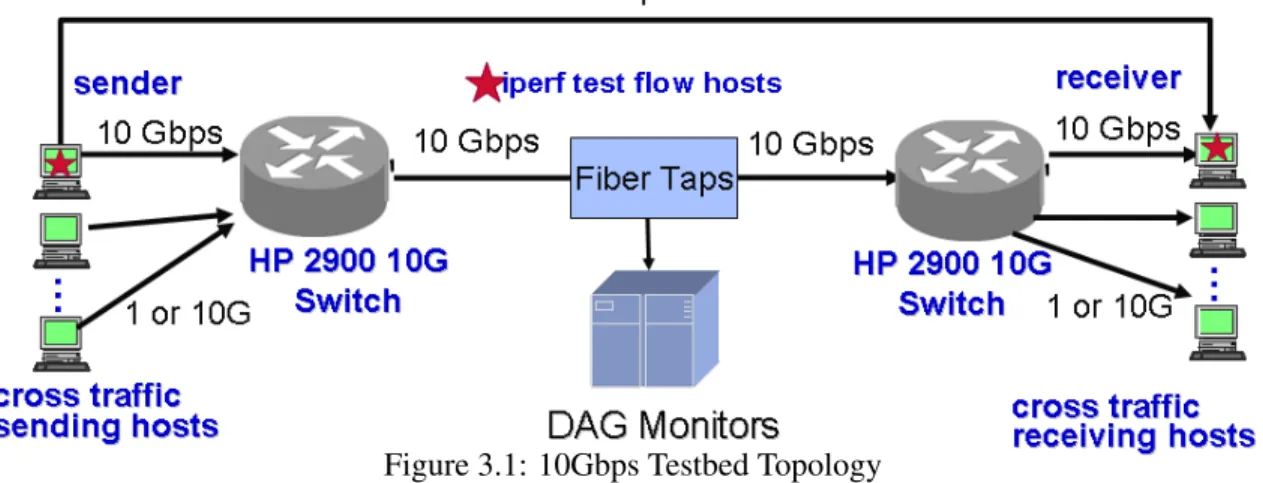
3.1 10Gbps Testbed Topology . . . 37
3.2 Throughput of Non-responsive Cross Traffic Every 1ms . . . 40
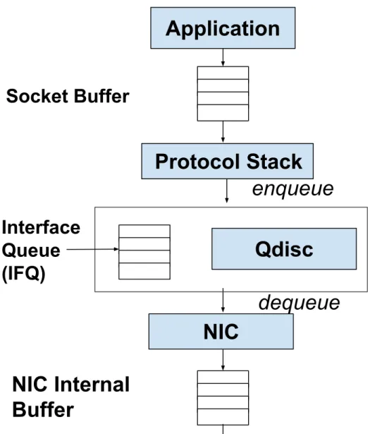
4.1 Network Buffering in Linux . . . 45
4.2 Use Gap-Packets to Create Gaps . . . 51
4.3 Inaccurate Gap Creation Using Dummy-packet . . . 52
4.4 Qdisc Packet Scheduler . . . 55
4.5 Gap Creation Errors . . . 58
4.6 Gaps withHrtimerat 4Gbps . . . 59
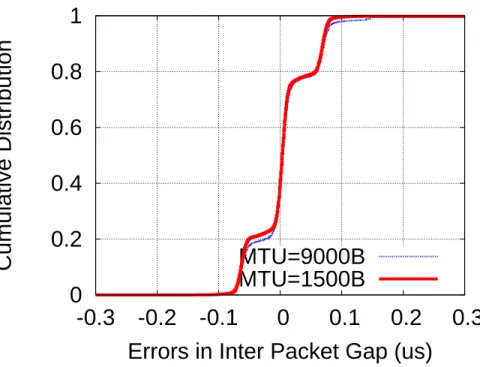
4.7 Gap Errors with Different MTU Sizes . . . 60
4.8 A Packet Group (Noise-free) . . . 61
4.9 Estimated Available Bandwidth . . . 61
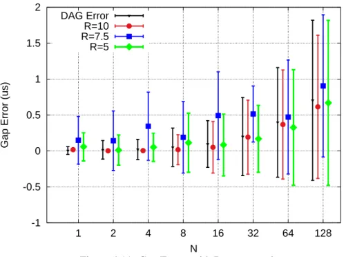
4.10 Gap-error with N Flows . . . 64
4.11 Gap Errors with Dummy-packet . . . 67
5.1 Bandwidth Decision Errors: State of the Art . . . 73
5.2 A P-stream Smoothed by IMR-Pathload . . . 75
5.2 A P-stream Smoothed by IMR-Pathload (cont.) . . . 76
5.3 State-of-the-Art: Impact of N . . . 77
5.4 Averaging with Various Window Sizes . . . 79
5.6 Bandwidth Estimation Error: PRC-MT + BASS . . . 82
5.7 BASS for a Multi-rate Probe Stream (avail-bw =6.8 Gbps) . . . 84
5.7 BASS for a Multi-rate Probe Stream (cont.) . . . 85
5.8 Multi-pass Spike Removal Reduces Over-estimation . . . 86
5.9 Impact of Probing Range . . . 89
5.10 Impact of P-stream Length . . . 91
5.11 Impact ofNr. . . 91
5.12 Impact ofGAP N S EP SILON . . . 92
5.13 Impact of AVG SMOOTH . . . 93
5.14 Impact of Delayed ACK . . . 93
6.1 Machine Learning Framework For Bandwidth Estimation . . . 98
6.2 Estimation Error of Single-Rate Probe Streams (N=64) . . . 101
6.3 Single-Rate Estimation Error Using BASS (Smaller N) . . . 103
6.4 Single-Rate Estimation Error Using Machine-Leaning (Smaller N) . . . 108
6.4 Single-Rate Estimation Error Using Machine-Leaning (Cont.) . . . 109
6.5 Multi-rate Estimation Error with BASS and Machine-Learning Models . . . 110
6.5 Multi-rate Estimation Error with BASS and Machine-Learning Models(Cont.) . . . 111
6.5 Multi-rate Probing with BASS and machine learning Models (Cont.) . . . 112
6.6 Impact of Cross-traffic Burstiness In Training and Testing, Respectively . . . 113
6.7 Probe Streams with DifferentICparam. . . 114
6.8 Impact of ICparams on NIC1 . . . 115
6.9 Interrupting Behavior on NIC2 . . . 115
6.10 Impact of ICparams on NIC2 . . . 116
6.11 Cross-Nic Validation . . . 117
7.1 Architecture of RAPID Implementation . . . 119
8.1 Decoupling Probing/Adapting . . . 126
8.2 Impact of Rate-Adapting Parameters with CBR . . . 130
8.4 Throughput with BCT every 1ms . . . 135
8.5 Duration of Web Traffic (RTT=5ms) . . . 140
8.6 Flow Duration of Web Traffic . . . 142
8.7 Throughput and Loss Rate of TCP Flow When Sharing the Path with Web Traffic . . . 143
8.8 Intra-Protocol Fairness . . . 145
8.8 Intra-Protocol Fairness (Cont.d) . . . 146
8.8 Intra-Protocol Fairness (Cont.d) . . . 147
8.8 Intra-Protocol Fairness (Cont.d) . . . 148
8.8 Intra-Protocol Fairness (Cont.d) . . . 149
8.8 Intra-Protocol Fairness (Cont.d) . . . 150
8.8 Intra-Protocol Fairness (Cont.d) . . . 151
8.8 Intra-Protocol Fairness (Cont.d) . . . 152
9.1 IMR-avg Estimation Error . . . 158
9.2 IMR-wavelet Estimation Error . . . 159
LIST OF ABBREVIATIONS AND SYMBOLS
TCP Transmission Control Protocol
ACK Acknowledgement
RTT Round Trip Time
OWD One-way Delay
NIC Network Interface Card avail-bw Available Bandwidth
sendgap Inter-packet Gap intended to be created at the sender recvgap Inter-packet Gap observed at the receiver side
CHAPTER 1: INTRODUCTION
1.1 Motivation
1.1 Issues with Loss-based TCP Congestion Control
TCP congestion control protocols were originally designed to reduce persistent network congestion, under which TCP flows suffer from massive packet losses and achieve extremely low throughputs. TCP congestion control protocols detect congestion on end-to-end paths and adjust TCP senders’ transmission rates to address the congestion; different protocol designs adjust the senders’ transmission rates differently. The original congestion control protocol, Tahoe, was designed in 1987; Tahoe and its successors, Reno, NewReno, and SACK, have been widely deployed for over three decades as the mainstream end-to-end congestion control mechanisms for the Internet.
These legacy congestion control protocols maintain a congestion window (cwnd) at the senders; this congestion window limits the number of packets that are unacknowledged during transfer to the number that can be sent within one round-trip time (RTT). The congestion control algorithms consist of two phases. In the first phase, after initialization, a TCP flow enters theslow-startphase, during which it aggressively doublescwndevery RTT; during this phase, no packet from the past RTT is lost. Oncecwndreaches some threshold (SS THRESH), the flow enters the second phase, thecongestion-avoidancephase; during this phase, it carefully and slowly acquires more bandwidth. In this second phase,cwndis updated based on the additive-increase and multiplicative-decrease (AIMD) principles: it is increased by one if there are no packet losses detected, and if packet losses are detected, it is reduced by half.
these new protocols adjustcwndmore aggressively in the congestion-avoidance phase [1, 3, 4, 5, 6, 7]. These methods have been shown to significantly improve path utilization on high-speed links with large RTTs [8]. But no matter how fast these protocols increase theircwnd, their performances are constrained by their loss-based congestion-control design: they rely on packet loss to infer the presence of network congestion. Packet loss is a binary congestion signal (either a packet gets lost or it does not), and it therefore does not reflect the degree of congestion on the network. Because packet loss offers limited feedback about the network status, protocol designers are more likely to design conservative congestion-control algorithms, rather than aggressive ones; loss-based control mechanisms must significantly reduce transmission rates after losses are detected in order to alleviate network congestion, and must increase transmission rates slowly enough to avoid repeated losses. As a result, loss-based protocols usually overreact to packet losses, wasting abundant network capacity. [2] has shown that even protocols [1, 5] designed for high-speed networks require hundreds of RTTs to regain full path utilization after a single loss on a 1 Gbps path. Packet loss is also a delayed indicator of congestion—loss-based protocols neither perceive congestion nor take action to ameliorate it until the congestion is bad enough to overflow the network buffers. To address congestion before it becomes critical, TCP protocols should use congestion signals other than packet loss.
1.1 Promises of Delay-based and Bandwidth-based Protocols
To address the drawbacks of loss-based congestion control, researchers have been actively looking for novel congestion indicators over the past decades. These efforts have led to two new types of congestion control protocols: delay-based and bandwidth-based protocols.
Delay-based Protocols
Some protocols using delay to signal congestion have been developed: these protocols measure an increase in either the one-way delay (OWD) or the RTT. When paths are congested, packets will be queued, and the queueing delay will increase OWD/RTT measurements. TCP protocols that infer congestion from RTT and/or OWD measurements are called “delay-based” protocols.
adjust their transmission rates by different degrees. These two features help delay-based protocols to reduce packet losses, achieve more stable path utilization, and increase fairness among competing flows [9, 10, 11].
Several delay-based protocols were developed in the 1990s and 2000s, including [9, 12, 13, 10, 14, 11]. During this period, many researchers also began to use delay measurements to enhance the performance of loss-based protocols [6, 15, 7, 16, 17, 18]. In 2015, the protocol TCP TIMELY [19] introduced delay-based protocol design to data centers for the first time.
Bandwidth-based Protocols
Instead of seeking alternative congestion signals, “bandwidth-based” congestion control methods identify congestion by directly probing for the transmission rate and comparing it to the maximum transmission rate that the path affords.1
Bandwidth-based protocols often borrow techniques from bandwidth estimators [20, 21, 22, 23] to probe the path for unused bandwidth, which is also known as available bandwidth (avail-bw). Bandwidth-based protocols adapt transmission rates to avail-bw; they are able to quickly identify and converge to changed bandwidth, and they can therefore utilize paths efficiently without causing excessive congestion.
Among existing bandwidth-based protocols (PCP [24], UDT [25], NF-TCP [26], and RAPID [2]), RAPID stands out for its performance, which is remarkably close to optimal on gigabit networks in NS2 simulations. It discovers and adapts to changing avail-bw within 1 to 4 RTTs; it ensures fair throughput among multiple RAPID flows with heterogeneous RTTs; and it has a negligible impact on legacy TCP flows sharing the path.
1.1 Hurdles to Widespread Adoption
Although delay-based and bandwidth-based protocols have demonstrated considerable performance gains over packet-loss protocols, there is significant resistance to their broad deployment across the Internet. Researchers seriously doubt whether these protocols’ performance in simulations or controlled testbeds can translate well to real-world settings, especially at ultra-high speeds, due to the following issues.
• Insufficient Timing Accuracy
packet arrival time and returns the timestamp to the sender in its acknowledgement. To accurately measure changes in delay magnitude, timestamps must be measured at finer granularity than queuing delay measurements. However, the necessary measurement granularity gets smaller as network speeds scale up. For example, on a 10 Mbps link with a frame size of 1500 B, the queuing delay is measured at scales of×1.2ms; an end-host with 1 ms timing granularity (jif f iesin Linux) can easily perceive queuing from these delay measurements. However, once the network speed scales up to 1 Gbps, the queuing delay scales down to×12µs—in this scenario, 1 ms is so coarse-grained that the same host will observe no queuing delay until the queue length reaches around 100. On even higher network speeds, of 10 Gbps and 40 Gbps, timestamping with at least1µsaccuracy is required.
Unfortunately, timestamping granularity is implementation-dependent. [27] shows that the majority of commercial servers only provide 10 ms–100 ms granularity —µ-scale resolutions are not available for most servers.
• Weak Correlation Between Delay and Congestion
Although delay-based and bandwidth-based protocols use delay measurements in different ways, all of them rely on the assumption that an increase in RTT or OWD is a strong sign of congestion. However, previous research [28, 29, 30] has shown that delay variations are only weakly correlated to path congestion, mainly because of transient queuing—packets arrive at routers in a very bursty manner [31, 32], and queues are built up and drained off at very short timescales. Because of this burstiness, packets may experience transient queuing even in the absence of congestion, and they may not be queued at all in the presence of congestion. Thus, increases in delay measurements cannot be relied upon to robustly indicate path congestion.
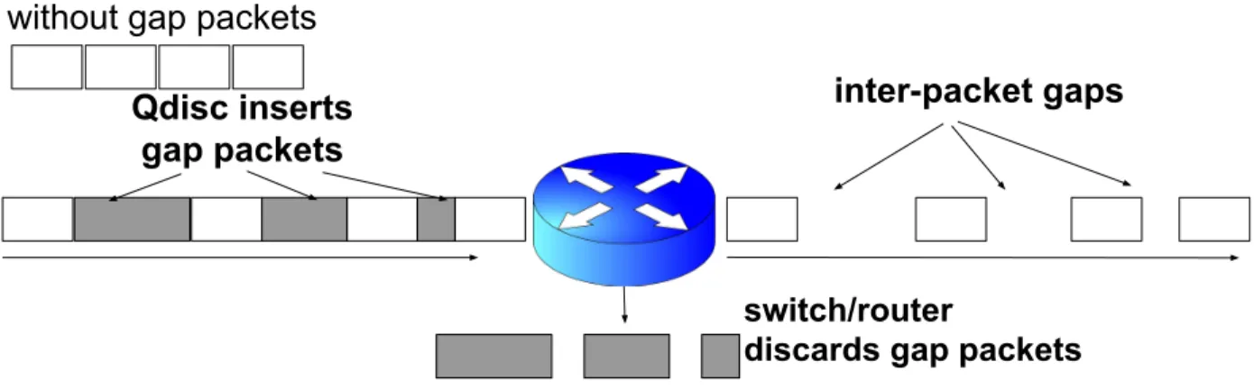
• Creating Inter-packet Gaps Is Challenging
6
8
10
12
14
10
20
50
60
Inter Packet Gap (us)
30
40
Probe Index
sendgap
recvgap
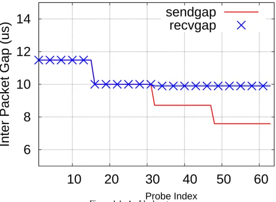
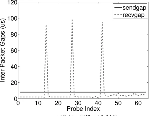
Figure 1.1: An Ideal p-stream
In noise-free networks, the inter-packet gaps at the receiver (recvgaps) are expected to be consistently larger than inter-packet gaps generated at the sending host once the probing rate starts to exceed avail-bw.
• Incompatibility with Existing Protocol Stack
Many protocols [14, 24, 25, 26, 2] also require the creation of time gaps between packets, or “inter-packet gaps.” In these protocols, “inter-packet transmission is “gap-clocked”—the transmission of each individual packet is determined by the time gap between it and the preceding packet. Unfortunately, this is a complete departure from widely deployed TCP protocol stacks, which couple packet transmission with ACK arrivals (“ack-clocked”). These new protocols inspire strong resistance—why would an operator of production servers get rid of a protocol that has been used for more than three decades in favor of a new protocol?
1.1 RAPID Stretches Challenges to Extreme
1.1 TCP RAPID —a Packet-scale Congestion Control Protocol
inter-packet gap between Ri and its previous packet, according to gis = RPi, whereP is the packet size
andgs
i is the time gap created by the sender between theith andi-1th packet. Each p-stream observes the inter-packet gaps when packets arrive at the receiver (denoted asgr) and compares them withgs. Bandwidth is estimated by searching for a signature ofpersistently increasing queuing delay: once the probing rate exceeds the avail-bw, inter-packet gaps keep increasing over the path due to persistent congestion. Therefore, avail-bw is the highest probing rate beyond whichgris consistently larger thangs. For instance, Fig 1.1 shows thegsandgrwithin a p-stream encountering 2.45 Gbps average cross-traffic on a 10 Gbps path that is free of noise;grbecomes consistently larger thangsafter the 33rd packet. In this scenario, theABestis the probing rate of the 32nd packet. Once the avail-bw is computed, RAPID updates the average transmission rate of the subsequent p-stream accordingly.
Mainstream protocols, whether loss-based, delay-based or rate-based, all control congestion by adjusting cwndsizes; the congestion control is reflected by thecwndincrement or by the reduction in the next RTT. In RAPID, every packet performs bandwidth probing, and every packet plays a key role in bandwidth estimation. To distinguish TCP RAPID from other congestion control methods, we refer to it as“packet-scale” congestion control.
1.1 Challenges in Practice
Perhaps even more than the existing delay-based and bandwidth-based protocols, RAPID encounters each of the above challenges to implementation.
• Delay-based protocols (e.g. Vegas and Fast) usually indicate congestion and react to it using the mean of all delay measurements within one RTT, rather than using every single delay sample. This averaging provides a denoising effect, alleviating the impact of noise caused by transient queuing and timestamping inaccuracy. However, our proposed packet-scale congestion control protocol usesevery inter-packet gap sample to estimate avail-bw, and accurate arrival timestamping foreverypacket is crucial.
• As mentioned in Chapter 1.1.3, scheduling packet transmissions based on inter-packet gaps is a key challenge on high-speed networks. Other rate-based protocols [24, 25, 26] create inter-packet gaps only intermittently, or use bandwidth probing and estimating merely as an enhancement to loss-based congestion control methods. In contrast,everypacket transmission in RAPID is “gap-clocked.” In other words, gap creation plays a crucial role in RAPID, which requires accurate throughput for the entire connection.
1.1 Goal of this dissertation
In this thesis, we ask the following question: can the challenges faced by delay-based and bandwidth-based protocols be addressed in real-world high-speed networks, enabling them to perform as well as promised? We explore this question using RAPID. If a protocol as demanding as RAPID can be put into use on ultra-high speed networks, that would be a convincing argument for the practical adoption of delay-based and bandwidth-based designs.
The goal of the thesis is thus to demonstrate how well RAPID performs in practice, and to test whether its real-world performance can match its outstanding performance in simulation. We identify challenges that prevent RAPID from delivering on its promises, address each of them with a novel or existing mechanism, and evaluate whether our Linux implementation meets performance claims in a 10 Gbps testbed. We also show that neither the challenges nor the mechanisms that address them are specific to RAPID; other delay-based and bandwidth-based protocols will also benefit from adopting those mechanisms.
1.2 Challenges of RAPID in Practice
In this section, we identify four challenges RAPID faces in implementations on high-speed networks. For each challenge, we briefly describe the requirement imposed by RAPID, the obstacles to achieving that requirement, and the way this thesis addresses the challenge.
1.2 Creating Accurate Inter-packet Gaps
1.2 RAPID Requirement
inter-packet gaps created at the sender. However, this kind of accuracy in gap creation is highly demanding. When probing high-speed networks, the required gaps are atµs timescales. For instance, in order to probe a 10 Gbps network, even with jumbo-sized frames, the spacing must be as small as a fewµs. A gap inaccuracy of even 1µs can lead to nearly 100% error in the intended probing rate.
1.2 Challenges
Creating such fine-scale, high-precision inter-packet gaps is fairly challenging for today’s end-hosts for two main reasons. First, modern operating systems are interrupt-driven; the gap-creation process can easily get interrupted, lose control of the CPU, and not be scheduled again before the gap time elapses. The resultant send gaps are unpredictable and imprecise. Second, before packets are transmitted to the outbound link, they can buffer at several places: (i) in the socket send buffer, when they are handed by the application to the kernel and are waiting to be processed by the TCP/IP protcol stack; (ii) in the interface queue associated with each outbound NIC; and (iii) in the NIC internal buffer when they are being transmitted out. Buffering puts packets back to back in the queue, closing up the inter-packet gaps.
1.2 Goal
The first goal of this thesis is to consider and evaluate techniques that create inter-packet gaps in order to find a mechanism that both ensures high-precision gaps and is resistant to interrupt and end-host buffering, and to tailor these techniques for RAPID.
1.2 Noise Removal to Achieve Accurate ABest
1.2 RAPID Requirement
Bandwidth estimation is the key component to RAPID, which searches for the signature ofpersistently increasing queueing delaywithin each p-stream. As described in Section 1.1.4.1, avail-bw is estimated as the highest probing rate before the signature is detected. RAPID’s robustness is based on the assumption that the inter-packet gap between thei-1th and theith packets expands if and only if the probing rate of theith packet
6
8
10
12
14
10
20
50
60
Inter Packet Gap (us)
30
4
0
Probe Index
sendgap
recvgap
Figure 1.2: p-stream after the bottleneck link
arrivals at routers are uniformly distributed and packets experience queueing delays only at bottleneck routers when congestion is present.
1.2 Challenges
On real-world networks, there are two types of noise sources that void the assumption that packets must experience increasing queueing delays if they keep probing at rates higher than avail-bw: burstiness at bottleneck resources and transient queueing at non-bottleneck resources.
• Burstiness in cross-traffic at bottleneck resources:
In a packet-switched network, traffic arrival can be fairly bursty at small timescales of 1 ms [?32], and this burstiness can introduce noise into the persistent queueing delay signature. Fig 1.2 illustrates the inter-packet gaps observed after the bottleneck link of a p-stream encountering the same avail-bw as in Fig 1.1. It fails to identify persistent queueing until the 49th packet.
0
20
40
60
80
100
10
20
50
60
Inter Packet Gap (us)
30
40
Probe Index
sendgap
recvgap
Figure 1.3: Probe Streams at the receiver
Inter-packet recvgaps present a “spike-dips” pattern due to interrupt coalescence at the receiving NIC.
Even a non-bottleneck resource can induce short-scale transient queues when it becomes temporarily unavailable because it is servicing competing traffic. This can happen, for instance, while accessing high-speed cross-connects at the switches, or while waiting for CPU processing after packets arrive at the receiver-side NIC.
0
0.2
0.4
0.6
0.8
1
0
10 20 30 40 50 60 70 80
Cumulative Distribution Function
Acknowledgement Processing Time (us)
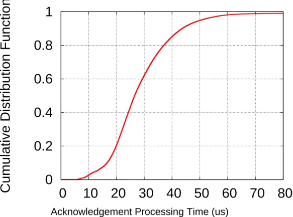
Figure 1.4: Processing Delay From a Packet Arrival to an ACK generated
to back and show negligible gaps. With interrupt coalescence, thepersistently increasing queueing delaysignature is completely unrecognizable. For every p-stream, avail-bw is estimated as the highest probing rate, leading to persistent overestimation.
1.2 Goal
Our second objective in this dissertation is to consider and evaluate techniques for reducing the impact of fine-scale noise in inter-packet gaps, which will help to achieve robust bandwidth estimation.
1.2 Stability/Adaptability Trade-off
1.2 RAPID Requirement
RAPIDrequires two features, adaptability and stability, for optimal functioning.
• Stability:However, RAPID should only adapt to avail-bw at a longer timescale; with relatively stable avail-bw, the longer timescale gives accurate results, and with highly volatile avail-bw, there is little point in adapting to anABestvalue that may have already changed drastically.
1.2 Challenges
Unfortunately, RAPID’s requirements for stability and adaptability cannot be simultaneously satisfied. After estimating avail-bw for each p-stream, RAPID then adjusts the average sending rate for the next p-stream based on the updatedABest. It uses the same timescale (given by the number of packets in each p-stream) to probe for avail-bw and to adapt to changes in avail-bw. Thus, there exists an intrinsictrade-offbetween the two timescales. The stability requirement favors longer p-streams, whose longer probing timescales are believed to be less impacted by noise and to yield more robustABest[35]. These longer p-streams also allow RAPID to adapt its transmission rate to a longer probing timescale, at which the avail-bw is stabler and less noisy. The adaptability requirement, however, favors shorter p-streams. A shorter probing timescale enables the protocol to sample avail-bw more frequently and track it more closely, as well as to respond more quickly to changes in network condition.
1.2 Goal
Our third goal is to design new mechanisms into the RAPID control algorithm that can alleviate the trade-off between stability and adaptability, allowing RAPID to track changes in avail-bw closely, yet to only adapt to avail-bw at stabler timescales.
1.2 Deployability Within TCP Stack
1.2 RAPID Requirement
struct tcp congestion ops{ · · ·
/* initialize private data (optional) */ void (*init)(· · ·);
/* return slow start threshold (required) */ u32 (*ssthresh)(· · ·);
/* do new cwnd calculation (required) */ void (*cong avoid)(· · ·);
/* call before changing ca state (optional) */ void (*set state)(· · ·);
/* call when cwnd event occurs (optional) */ void (*cwnd event)(· · ·);
/* call when ack arrives (optional) */ void (*in ack event)(· · ·);
/* hook for packet ack accounting (optional) */ void (*pkts acked)(· · ·);
};
Figure 1.5: The Linuxtcp congestion opsInterface 1.2 Challenges
Ensuring that the RAPID implementation integrates seamlessly with existing protocols and servers is a significant challenge for two reasons, which will be explored in the next two sections of this thesis.
1.2 “gap-clocking” vs “ack-clocking”
RAPID’s packet-sending process is fundamentally different from that of the state-of-the-art TCP. Since Linux is the most widely used open-source system, and the system upon which all TCP protocols except Compound are tested, we use the Linux TCP packet-sending process as an example to illustrate the difference between RAPID and TCP. In Linux, the packet-sending process is “window-controlled” and “ack-clocked.” The “window-controlled” aspect means that a sliding window ofcwndsize is maintained for outstanding packets. The “ack-clocked” aspect couples the receiving of ACKs with the transmission of new packets; once an ACK for the 1st packet in thecwndarrives, TCP updatescwnd, advances the sliding window, and sends more packets, for as long ascwndallows.
The current Linux kernel provides a congestion handler interface (tcp congestion ops) that implements various congestion control protocols in a pluggable manner (Fig 1.5 lists all interfaces). Usingcong avoid, it allows changes to the amount by whichcwndchanges when ACKs are received, but it provides no method of controlling when a packet is sent out. Clearly, to support “gap-clocking,” Linux needs modules beyond the TCP congestion control framework. Instituting support for gap-clocking would not only support RAPID; other protocols that rely on bandwidth estimation, even intermittently, also require “gap-clocking” to be realized.
1.2 Fine-scale Arrival Timestamping
In order to calculate avail-bw at ultra-high speeds, the timestamps of packet arrivals must be observed by the RAPID receiver, and communicated back to the sender, atµs levels of precision. It is intuitive to use the timestamp fields in TCP headers to communicate packet arrival times; once the receiver finds that the TSval field is set in a packet header, it echoes that value in the TSecr in the returning ACK, and writes the ACK generation time in the TSval field. However, the granularity of TCP header timestamping is implementation dependent, ranging from 500 ms to 1 ms [27]. Linux can provide accuracies of only 1 ms—a granularity that is still much coarser than the inter-arrival gaps, which are measured atµs timescales. With such coarse granularity, the inter-arrival gaps become straight 0s. Moreover, timestamps are produced when ACKs are created, rather than when the respective packets are received. This belated timestamping means that gaps are subject to variable ACK processing times. Fig 1.4 plots the time difference between packets’ actual arrival times—the times when packets are handed from the receiving NIC to the receiver OS—and the value recorded in TCP timestamps in the returning ACKs. We find that the two can differ by up to 60µs.
The high-precision timing requirements of RAPID packet arrivals require some mechanism beyond simply relying on TCP timestamping.
1.2 Goals
1.3 Thesis Statement
Because of its continual bandwidth probing and adapting, TCP RAPID extends the practical challenges faced by other delay-based and rate-based protocols to extreme levels. By carefully addressing each of these challenges, the performance demonstrated by RAPID in previous simulation-based work is deliverable in real-world networks.
1.4 Contributions
This thesis investigates mechanisms to address each of the identified challenges faced by packet-scale congestion control protocols in real networks. In the following sections, we summarize the key contributions of this thesis.
1.4 Creating Accurate IPGs
We survey and evaluate several state-of-the-art methods of creating inter-packet gaps using only software. We find that the method used in PSPacer [36] is able to create inter-packet gaps on 10 Gbps links with errors of less than 0.5µs.
1.4 Denoising for Accurate Bandwidth Estimation
1.4 Addressing the Stability/Adaptability Trade-off
To address RAPID’s trade-off between stability and adaptability, we decouple the probing timescale from the adapting timescale. Instead of updating the average transmission rate of p-streams for every avail-bw estimate made, RAPID is set to probe avail-bw with shorter p-streams and to adapt its sending rates to the mean of the latestγbandwidth estimates only everyγp-streams.
1.4 Implementing on Standard Protocol Stacks
We develop mechanisms to realize gap-clocking at the sender and microsecond-resolution packet timestamping at the receiver within standard Linux protocol stacks.
1.4 Realizing gap-clocking
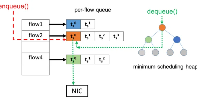
To realize gap-clocking, we design a packet scheduler in the link layer that shares some data structures with the TCP module. It groups packets in the interface queue into p-streams, computes inter-packet gaps based on the average sending rate computed by the TCP module, and sends packets to the outbound NIC according to inter-packet gaps .
1.4 Achieving Fine-scale Arrival Timestamping
To timestamp packet arrivals with at leastµsaccuracy, we develop a set of packet-scheduler modules: two modules at the receiver (one to timestamp incoming packets withµs resolution and another to replace this high-resolution timestamp in the ACK TSval field before ACKs are sent out), and one module at the sender (to record the timestamp in the returning ACKs and replace it with thems-resolution value to ensure proper TCP header processing).
1.4 Evaluation of RAPID in Ultra-high-speed Testbed
Incorporating the previously mentioned mechanisms, we implement RAPID as pluggable kernel modules in Redhat Linux 6.7 with kernel version 2.6.32. Specifically, we
• decouple the probing timescale from the adapting timescale withX= 3; and • use three packet-scheduler modules for timestamping withµs accuracy.
We evaluate this implementation in our 10 Gbps testbed and compare its performance to that of other congestion-control protocols, and we find that our implementation lives up to its performance in simulations: it is adaptive to random packet losses and to bursty cross traffic, consistently providing higher throughputs than other protocols while remaining non-intrusive to coexisting conventional TCP flows.
We then test which of these mechanisms has the strongest effect on the RAPID implementation by removing them one by one and repeating the previous evaluations without each one. We find that each of these mechanisms is crucial: RAPID’s performance gains cannot be achieved without all four of the mechanisms in place.
1.4 Apply the Lesson to Other Delay- and Rate-based Protocols
We adapt the mechanisms designed for RAPID to other delay-based and rate-based protocols. Specially, for TCP Vegas we measure RTTs at a finer-grained level by recording packet arrivals with the Qdisc mentioned in 1.4.4; we also use the “Dummy-packet” mechanism to reduce traffic burstiness for TCP pacing, We find that these mechanisms also help other delay- and bandwidth-based protocols deliver better performance that is adaptable to real-world high-speed networks.
1.5 Outline
CHAPTER 2: BACKGROUND
This chapter provides background knowledge that is related to this thesis, including basics and evolution of TCP, RAPID congestion control algorithm that was proposed in its original paper [2], common methods of bandwidth estimation, and the brief introduction of machine learning algorithms that are mentioned in this thesis. Readers familiar with this background can skip this chapter.
2.1 Historical Perspective of TCP Congestion Control
In this section, we briefly review the evolution of TCP transmission control protocol in the past decades, focusing on its congestion control algorithm. We first describe the functionality of TCP congestion control, discuss its deficiency in newer high-speed networks, and introduce state-of-the-art solutions to address it.
2.1 Transport Control Protocol
Computer networks are often described using a layered conceptual model. TCP/IP reference model is the most widely accepted model by industry, which abstracts the network into four layers. From top to down, they are: application layer, transport layer, internet layer, and network access layer. Each layer uses some protocol— a set of rules regarding the procedures that two entities communicate with each other — to carry out different functionalities. In the topmost application layer, applications exchange information between remote end-hosts according to application protocols to perform specific tasks, e.g. file transmission (which uses FTP protocol), and solving domain names (which uses DNS protocol). Protocols of transport layer are responsible for delivering data between the two application processes on the two end-hosts. Protocols of Internet layer are responsible for delivering data from the sending host to the receiving host over the Internet. The network access layer moves data without error on the physical link between two directly-connected hardwares. The upper-layer protocol relies on the functionality provided by the layer below it.
end-to-end (from the sending host to the receiving host) connection. It provides reliably transmission using its loss-recovery mechanism — if the receiver fails to acknowledge the sender on the receipt of a packet within a certain amount of time, the sender immediately retransmits that packet, and repeats this process until this packet is acknowledged. Besides, it employs mechanisms that react to network congestion (which will be described in Section 2.1.2). The congestion control mechanism allows each connection to detect congestion and slow down transmission accordingly, preventing the Internet from “congestion-collapse”, where each connection experiences losses repeatedly due to persistent congestion, and fails to transmit data efficiently. TCP has been extensively utilized by many popular applications such as web, email, file sharing and video streaming. According to the monthly report by Caida [37], TCP carries the majority of total traffic on the current Internet backbone nowadays.
2.1 Loss-based Congestion Control
Network congestion occurs when the intermediary devices on the path, i.e. switches and routers, receive data packets faster than they can process. Packets are buffered in the internal queues of these devices, waiting to be served. Packet loss is a deterministic consequence of persistent congestion — with the queue building up, further incoming packets are discarded once the queue overflows.
The legacy TCP congestion control protocol (Tahoe, Reno, and New Reno) regards packet-loss as the indicator of network congestion, and developed an additive-increase and multiplicative-decrease (AIMD) strategy to react to it. We briefly describe the strategy as follows.
The AIMD strategy relies on the notion of congestion window (cwnd ), which sets the upper bound of packets that can be in flight (unacknowledged) at any time. In other words, within each RTT, only a
cwndworth of packets can be sent. The data transmission process consists of two phases — the connection entersslow-startphase in the beginning of the transmission, wherecwndis aggressively incremented by 1 upon every acknowledgement; once a packet-loss is detected, the connection halvescwnd, and switches to congestion-avoidancephase, wherecwndis gradually increased by cwnd1 upon each acknowledgement.
utilization. To address the issue, new protocols have been proposed that behave more aggressive in both slow-start and congestion-avoidance phase than AIMD — BIC, Cubic, HTCP, HighSpeed, and Scalable are prominent examples of them. These protocols have been reported to improve link utilization on highspeed links, and have been deployed in the Linux kernel protocol stack. We refer to these congestion-control protocols that only respond to packet-loss as “loss-based”, and briefly describe the algorithms of those loss-based protocols used in the test-bed evaluation in Chapter 8.
2.1 NewReno
TCP NewReno was developed upon earlier TCP protocols Tahoe and Reno with a more efficient loss-recovery mechanism. It was standardized by IETF in 2004 [38], since then has been referred to as the standard TCP. Its congestion control inherits the AIMD strategy:
cwnd=
cwnd+ 1 , upon a receipt of acknowledgement in slow start phase
cwnd+cwnd1 , upon a receipt of acknowledgement in congestion avoidance phase cwnd
2 , upon a loss detected by duplicate acknowledgements
(2.1)
Its effect is thatcwndgets doubled in slow-start phase, and only increased by 1 in congestion-avoidance phase.
2.1 BIC
2.1 Cubic
The binary search technique can be too aggressive for TCP on low-speed networks, which tends to cause repeated packet losses. To address this issue, TCP uses a new cubiccwndgrowth function as follow:
cwnd =c×(t−K)3+cwndmax (2.2)
where t is the elapsed time since the last window reduction after packret loss,K =q3 cwndmax×ρ
C , and C is a scaling factor. Similar to BIC, it denotes thecwndbefore a packet loss occurs ascwndmax. After a window reduction by half after loss, Cubic grows itscwndrapidly. When it gets closer tocwndmax, it slows down the increasing trend —cwndincrement becomes zero at whencwnd =cwndmax. After that,cwndgrows in a reverse fashion, probing more and more boldly towards even higher rates. [5] has shown that Cubic enhanced the stability and link utilization of BIC, and also highly scalable at high-speeds. Cubic has been the default congestion control protocols since Linux kernel 2.6.19.
2.1 HighSpeed
For legacy TCP, thecwndreduction after packet loss is always proportionally to thecwndvalue before loss occurs — the largercwndgrows to, the more drasticallycwndgets reduced. HighSpeed TCP [1] made a sharp observation that such severe reduction is unnecessary whencwndis large, which often indicates that the network capacity is high. Instead, with a largercwnd, the flow should behave more aggressively to quickly grab the abundant bandwidth resource after packet loss. HighSpeed modifies thecwndgrowth at each acknowledgement as follows:
cwnd=
cwnd+cwnda(w) , congestion avoidance (1−b(w))×cwnd , upon loss
(2.3)
2.1 Scalable
Like HighSpeed, Scalable TCP [3] also aims to makecwndgrow more quickly than the one packet per RTT, as well as to improve the loss recovery time. It also has a thresholdcwndsize, below which Scalable TCP reconciles to the legacy TCP. Whencwndincreases beyond that threshold, Scalable updatescwndas follows upon every packet acknowledgement:
cwnd=
cwnd+ 0.01 , congestion avoidance
cwnd−0.125×cwnd , upon loss
(2.4)
The congestion window is increased by 1% of the currentcwndvalue each RTT, and reduced less drastically after loss is detected.
2.1 Hybla
In both slow-start phase and congestion avoidance phase of legacy TCP, thecwndincreasing rate is inversely proportional to RTT. This penalizes long-RTT flows with lower throughput when sharing paths with short-RTT flows, especially for those terrestrial satellite traffic where RTTs can reach 500ms and losses can be frequent due to terrestrial link errors. TCP Hybla [10] specifically targets at this issue for satellite flows, and proposes to remove performance dependence on RTT using the following algorithm:
(RT T
RT T0
)2× 1
cwnd +cwnd (2.5)
RT T0is a reference value used for all Hybla connections. The Hybla mechanism allows satellite traffic to
increasecwndat a rate proportional to RTT, significantly reducing the performance disparity against these long-RTT flows.
2.1 Delay-based and Rate-based Congestion Control
introduced the efforts of using queuing delay and available bandwidth as alternative congestion indicators to address the issues of loss-based design. In this section, we describe the congestion control algorithms of the protocols used in the evaluation in Chapter 8. Among them, TCP Vegas is a truly delay-based protocol which solely relies on delay to perform congestion control in congestion-avoidance phase. Other protocols, namely, Hybla, H-TCP, Illinois, Yeah, Fast and Compound, follow a hybrid of delay-based and loss-based approaches.
2.1 Vegas
TCP Vegas was developed in 1994 [9], which first introduced delay as congestion indicator. The designer of Vegas pointed out that congestion can be detected in an earlier stage before triggering packet-loss. When a network path starts to congest, packets are queued for longer in the network queues, leading to larger RTTs. Thus, earlier congestion can be observed by whether RTTs packets experienced increase. Vegas keeps track of the minimum RTT throughout the transfer asbaseRT T, computes the minimum RTT observed during the past round-trip time asminRT T, and updatecwndas follows:
dif f =cwnd−cwnd×baseRT T
minRT T, (2.6)
cwnd=
cwnd+ 1 , ifdif f < α cwnd , ifα≤dif f ≤β cwnd−1 , ifdif f > β
(2.7)
Ifdif f is less thatα, Vegas regards the path as non-congested, and increasescwndlinearly as NewReno does. Oncedif f goes beyondα, it signals possible congestion on the path, and Vegas stopscwndgrowth. A
dif f value larger thanβ indicates severe queuing delays, which is a definite sign of path congestion. In this case, Vegas linearly reducescwnd. [9] reported that Vegas achieved higher throughput than NewReno on congested links, due to its earlier congestion detection which avoided many packet loses.
2.1 H-TCP
Hamilton TCP [39], or H-TCP for short, uses delay to determine the amount ofcwndreduction once packet-loss is detected — rather than halvingcwnd, it is reduced by a fraction of RT Tmax
2.1 Illinois
The idea of TCP Illinois [17] is to use AIMD strategy, but adopts delay as a secondary congestion signal to determine the amount ofcwndincrement and decrement — once queuing delay experienced by packets increases, thecwndincrement rate should decrease, and reduction-rate after loss should increase, and vice versa. Illinois maintains a variabledaas the average queuing delay experienced by packets within one RTT, and updatescwndas follows:
cwnd=
cwnd+αcwnd(da) , congestion avoidance
cwnd×(1−β(da)) after loss
(2.8)
whereα(da)andβ(da)are functions of the queuing delay:
α(da) =
αmax , if da≤d1 k1
k2+da , otherwise
β(da) =
βmin , if da≤d2 k3+k4×da , d2≤da≤d3
βmax , otherwise
(2.9)
where d1, d2 and d3 are pre-defined thresholds. Thus, in congestion avoidance phase,cwndincrement rate is a reciprocal function of queuing delay; after packet loss,cwndreduction rate increases linearly with queuing delay.
2.1 Yeah
Scalable TCP has been shown to efficiently use high link utilization, but may starve NewReno flows sharing the network path. TCP Yeah [7] attempts to maintain the advantage of Scalable, and avoid its disadvantage. It uses two modes, fast mode and slow mode. In fast mode, Yeah behaves in the same manner as Scalable, while in slow mode it behaves as NewReno. The watershed of two modes are the queuing related variablesLandQ.L= RT T
baseRT T, which indicates the extent of average queuing delay experienced by acwnd worth of packets. Q= ( RT T
2.1 Westwood
TCP Westwood [40] aims at improving the behavior of NewReno after packet losses — the halving of cwndis too drastic and leads to low link utilization in loss recovery phase, especially on wireless links where losses are not induced by congestion but by link errors. Westwood proposes to set transmission rate to the available bandwidth avail-bw on the path when loss occurs. Westwood estimates avail-bw as the returning rate of acknowledgements before loss is detected — this rate is equal to the receiving rate at the receiver, which indicates the maximum rate the flow is able to achieve. This mechanism allows Westwood to maintain high efficiency after losses without causing excessive congestion, and has shown be significantly improve path utilization on lossy links [40].
2.1 Veno
TCP Veno [41] is a synthesis of Vegas and NewReno designs. For each RTT, Veno maintains a variable
dif f the same as Vegas, and usesdif f to determine the amount ofcwndincrement:
cwnd=
cwnd+ 1 , ifdif f ≤β cwnd−0.5 , ifdif f > β
(2.10)
The above mechanism makescwndgrowth less aggressive than NewReno when queuing delay continues to increase.
On wireless links, packet losses may not be caused by congestion, but by wireless link errors. In this case, halvingcwndas NewReno does is unnecessary and leads to low link utilization. One highlight of Veno design is that it tries to distinguish the causation of packet-losses on wireless links, with the aid of delay — ifdif f is smaller thanβ when the loss occurs, the path is non-congested and the packet-loss regarded as caused by link errors; otherwise, the loss is caused by congestion. In the former case,cwndis reduced by only 20% after loss, and 50% for the latter case.
2.1 TCP LP
through monitoring one-way delays for every packet. TCP LP removes the slow-start phase of NewReno, but starts with additive-increase phase which increasescwndby 1 every RTT. Once the average one-way delay in one RTT exceeds the minimum delay observed, LP regards the path in congested state, and conducts multiplicative-decrease which reducescwndby half.
2.1 Fast
Fast TCP [11] is a delay-based protocol, which aims at maintaining fixed-queue utilization for each flow. It computes RTT for every packet, and maintainsbaseRT T as the minimum RTT observed. At regular short intervals,cwndis updated via the following weighted average:
cwnd(T) = (1−γ)×cwnd(T −1) +γ×(baseRT T
RT T ×cwnd(T−1) +α) (2.11)
wherecwnd(T) is the computedcwndvalue for te T-th interval,γis a constant between 0 and 1, andαa constant integer. The effect of the abovecwndupdate mechanism is at any time the maximum queue size on the path isα. [11] and [42] have shown that Fast helps to achieve high throughput as well as better flow stability on high-speed links.
2.1 Compound
Compound TCP maintains two congestion windows — a loss-based windowWlossand a delay-based windowWdelay. The effectivecwndis the sum of these two. In congestion avoidance phase, theWlosswindow is updated in the same way as NewReno, which increases by W 1
loss+Wdelay for each acknowledgement; while Wdelay is derived from TCP Vegas. Compound TCP has been adopted by default in Windows systems since the release of Vista in 2008.
2.2 Bandwidth Estimation Techniques — PRM
Bandwidth estimation is a key component in many domains. It is used in congestion control protocols, e.g. RAPID, NF-TCP, UDT and PCP [26, 25, 24] to directly estimate avail-bw.
elect a proper server for each user for best user experience. The past decade has witnessed a rapid growth in the design of techniques for estimating available bandwidth [23, 21, 20, 22, 33]. In this section, we introduce the basic techniques for bandwidth-estimation that are widely used in existing tools.
2.2 PRM-based Bandwidth Estimation
Existing bandwidth estimation techniques base their estimation logic on two prominent models, namely, the probe gap model and the probe rate model (PRM) [23]. Tool evaluations have shown that PRM tools are more robust in the presence of multiple congested links [44, 45]. As a result, RAPID employs PRM in its bandwidth estimation logic. Below, we briefly summarize the PRM approach.
PRM tools typically send multiple packets at the same probing rate, in groups commonly referred to as p-streams—probing rate,ri, of theith packet is achieved by controlling the inter-packet gap as: gsi =
pi ri,
wherepiis the size of theith packet andgisis the gap between packeti−1andi. We useN to denote the length of a probe-stream, in terms of number of packets.
2.2 the principal of “self-induced congestion”
PRM tools base their bandwidth estimation logic on the principle of“self-induced congestion”— packets are expected to experience longer and longer queuing delays if they keep arriving at the bottleneck link at a higher rate than the available bandwidth. According to this principal: ifri >avail-bw, thenqi> qi−1, where
qi is the queuing delay experienced by theith packet at the bottleneck link, and avail-bw is the available bandwidth on that link. Assuming fixed routes and constant processing delays, this translates togr
i > gsi, wheregr
i is the gap observed at the receiver between theith andi−1th packets.
Most tools send out multiple packets at each probing rate, and check whether or not the receive gapsgr are consistently higher than the send gapsgs. They try out several probing rates and search for the highest rate rmaxthat doesnotcause self-induced congestion. Thisrmaxis then regarded as an estimate of bandwidth on the path.
2.2 Feedback-based Single-rate Probing:
The sender relies on iterative feedback-based binary search to find thermax. Starting with a probing range
{Rmin,Rmax}, the sender sends all packets within a p-stream at the same probing rateR = Rmin+2Rmax, and waits for receiver feedback on whether the receive gaps increased or not. If such signature of self-induced congestion is found, the sender updatesRmax asR; otherwise, it setsRmintoR. The process is repeated untilRminandRmaxconverges (Rmax−Rmax < ).
Pathload Pathload is the most prominent of such tools [20]. IMR-Pathload [33] mentioned in Section 5.1 rely on Pathload to estimate avail-bw. Here we briefly describe its estimation logic.
Pathload sends p-streams of 100 packets within each, and every packet probes for an identical prob-ing rate R. One-way delays for every packet are observed — we denote them as a vector D =< delay1, delay2, ..., delayN >. D is then fed into two trend-detection tests, namely, PCT and PDT, to detect whether an increasing trend of one-way delays exhibit.
PCTstands for pairwise comparison test, which tests the fraction of consecutive one-way delays that are increasing. PCT computes a metricSP CT: SP CT =
PN
k=2(I(delayk>delayk−1))
N−1 , whereI(delayk> delayk−1)
is 1 ifdelayk > delayk−1is true, otherwise this term is 0.
PDTstands for pairwise difference test, which quantifies how strong is the start-to-end one-way delay variation, relative to the one-way delay absolute variations for each pair of consecutive packets. It computes the metric ofSP DT:SP DT = PN delayk−delay1
k=2|delayk>delayk−1|.
IfSP CT >0.66andSP DT >0.55, then the p-stream is regarded as strongly exhibiting signature of self-induced congestion, and consequently its probing rate exceeds avail-bw. IfSP CT <0.54andSP DT <0.45, then the p-stream is free of self-induced congestion, andRmust be smaller than avail-bw. Otherwise, whether
Rexceeds avail-bw or not is regared as “ambiguous”.
2.2 Multi-rate Probing
The sender usesmulti-rateprobing without relying on receiver feedback — each pstream includes
N = Nr×Np packets, where Nr is the number of probing rates tried out. The sender looks for the highest probing rate that did not result in self-congestion. Fig 1.1 illustrates a multi-rate pstream with
probing facilitates the design of light-weight and quick tools, which transmits a smaller number of packets and estimates using much less time [45]. PathChirp is the most prominent of such tools [22], whose algorithm is described in Algorithm 1. TCP RAPID adopts this algorithm for bandwidth estimation on multi-rate p-streams.
Algorithm 1pathchirp abest(gs,gr, GAP NS EPSILON)
1: m=i=1, L=4
2: fork in 1 to N:ABk= 0
3: whilei < N j = i+1
4: whilegrj ¿gir+ GAP NS EPSILON
5: j+ +
6: ifj−i+ 1>=L
7: fork in m to j:ABk=Ris−1
8: i=m=j+1
9: else
10: i=i+ 1 11: return avg(ABi)
2.3 TCP RAPID
In this section, we describe the congestion-control algorithm of our targeted protocol, TCP RAPID. Instead of simply relying on packet loss as congestion feedback, RAPID is a bandwidth-based protocol — it continuously sends packets out in logical groups referred to as p-streams to estimate avail-bw, and then uses the estimates to guide the transmission rate of following p-streams. The congestion-control mechanisms consists of three components operating in a closed loop (Fig 2.1). Given an average send rateRavg informed by therate adapter, thep-stream generatorsends packet out in units of p-streams. Once the ACKs for a full p-stream return, thebandwidth estimatorcalculates the end-to-end avail-bw, based on which therate adapter updates the sending rate for the next p-stream.
Pstream Generator
Rate Adaptor
Bandwidth Estimator
Pstream Generator avail-bw
Ravg
<gs, gr>
packets out ACK in Figure 2.1: TCP RAPID Architecture
some rate R, by controlling the send-gap (gs) from the previous packet sent as: gs = PR. Within a p-stream, packets are sent atNrdifferent exponentially-increasing rates (withNppackets sent at each rate): Ri =Ri−1×s, i∈[2, Nr], s >1. Fig 1.1 plots the gaps in an intended p-stream withNr= 4, andNp= 16. The average send rate of the full p-stream is set toRavg, informed by the rate adapter.
Bandwidth Estimator
The mission ofbandwidth estimatoris to obtain an estimate for each fully-acknowledged p-stream, by observing queuing delays experienced by each packet within it.
The RAPID receiver records the arrival time of data packets and sends back the timestamps in ACKs. Once the sender receives all ACKs for a p-stream, it extracts these timestamps, computes the receive gaps (gr), and feeds them to the bandwidth estimator. The send and receive gaps for those multi-rate p-streams, gsandgr, are used to compute an estimate for the end-to-end avail-bw based on the algorithm described in Section 2.2.1.3.
Rate Adapter Ravgis initialized to 100Kbps. Thereafter, every timeABestis updated, the average sending rate of the next p-stream is also updated by applying a conditional low-pass filter as:
Ravg =
Ravg+τl ×(ABest−Ravg), ABest≥Ravg Ravg−η1 ×(Ravg−ABest), ABest < Ravg
wherelis the duration of the p-stream , andτ andηare constants. The effect of the above filter is that it takes aboutτ time unitsforRavg to converge to an increased avail-bw, andηp-streams to converge to a reduced avail-bw.
The low-pass filter enables RAPID to simultaneously achieve two desirable properties. First, by setting
Ravg lower than estimated avail-bw, it prevents RAPID to transmit at a higher speed than the network can currently handle. Meanwhile, within a single p-stream packets probe for rates both higher and lower than
2.3 Performance Promises in Simulation-based Evaluations
[2] evaluated the performance of RAPID in NS2 simulation on a 1Gbps testbed, and demonstrate that RAPID has close-to-optimal performance along several dimensions, most notable of which are:
• discovering and adapting quickly to changes in avail-bw within 4 RTTs;
• maintaining high link utilization throughput closely tracking and adapting to changes in avail-bw; • having low-queuing profile at switches/routers on the bottleneck link;
• being highly friendly to low-speed legacy TCP flows.
However, the related experiments were completely conducted in simulation environment, which is free of real-world noise. To be specific, the pstream generator is able create perfect inter-packet gaps , the cross-traffic is highly smooth, and thebandwidth estimatoris guaranteed to estimate avail-bw precisely. Whether these properties can be translated into real-world situation is questionable, and is to be explored in this thesis.
2.4 Machine Learning Algorithms
In Chapter 6 we develop a machine-learning based methodology to estimate available bandwidth. In this section, we introduce basic concepts of machine learning, as well as those machine-learning algorithms mentioned in Chapter 6.
Machine Learning Algorithm
learned model
feature vector: x=<x1,x2,...,xp>
<Xtrain, Ytrain>
<Xtest, Ytest> Evaluate
Yest
Training Phase
Testing Phase
Figure 2.2: Machine Learning Training and Testing Phases
2.4 Classification and Regression
Machine learning is commonly used to solve two types of problems, Classification and Regression. Classification is the problem of identifying new observations into a known set of categories. For instance, to classify whether an incoming flow is malicious or not [49] is a classification problem, which matches a flow into two categories. Different from classification, there exists no known “buckets” for the output of regression. Rather, the aim of a regression problem is to “generate” a discrete number for a new observation, based on the relationship between existing observations it discovers. For example, predicting future trend of a stock based on its transaction history [48] is a regression problem.
2.4 Training and Testing
For both classification and regression problems, machine-learning aims to figure out the relationship between inputx, and outputy.x= (x1, ..., xp), often referred to as a feature vector, consists of p features that are believed to relate toy. For instance, to learn the stock price based on monthly history, the outputyis the price fordayi, and the inputxis the vector of daily price for the past month fromdayi−30todayi−1.
Y, and then to generate a learned “model” to mathematically represent the relationship. The testing phase tests the quality of the learned model against a testing set< Xtest, Ytest >, which contains observations that not excluded from in the training set. The model takes inXtest, and computes the estimated resultYest. Its performance is evaluated by comparingYestwith the ground-truthYtestin the testing set.
It is commonly acknowledged that a training set that contains large enough samples and has a good coverage of diversity in the inputs features, is helpful to generate a more accurate model [54].
2.4 Machine Learning Algorithms
In Chapter 6 several popular machine-learning algorithms are adopted to improve the performance of RAPID bandwidth estimator. In this section we describe the basic ideas of their learning processes, without diving into the algorithmic details, which is out of the scope of this thesis.
ElasticNet ElasticNet [55, 56] is one of the most prominent linear-regression algorithms, which assume a linear relationship between input vectorXand outputY as follows: Y =wo+ ΣPi=1wixi. The aim of a linear-regression algorithm is to tune the linear coefficientswiin order to minimize the model error against the training set.
RandomForest
RandomForest, AdaBoost and GradientBoost all base their learning algorithms on decision tree method. Each decision tree solves a classification function. It regards the input vector x = (x1, ..., xp) as a p-dimensional space, partitions the space into a set of regions, each corresponds to an outputyin the training set. Thenxin the testing phase is mapped into a region, whose output the correspondingyin that region.
RandomForest generates a model that consists of multiple trees. Each tree model is trained with a randomly selected subset of training data.The output of the ultimate model is the average of the output of all tree models.
AdaBoost
Similar to RandomForest, AdaBoost relies on learning a number of decision tree models. However, unlike RandomForest for which each regression tree model is trained on a subset of training set, each tree for AdaBoost is to fit the entire training set and all features.
data samples that it fails to classify correctly. When the subsequent tree model is built, it focuses on fixing those miss-classified data samples.
The output of the final model is the weighted sum of the output of all tree models, the weight of each is determined during the learning process. The model produced by such “boosting” method is considered to be more accurate than RandomForest [57, 58].
GradientBoost