Analysis of a new spatial interpolation weighting method to estimate missing data applied to rainfall records

© 2019 Universidad Nacional Autónoma de México, Centro de Ciencias de la Atmósfera. This is an open access article under the CC BY-NC License (http://creativecommons.org/licenses/by-nc/4.0/).

Analysis of a new spatial interpolation weighting method to estimate missing

data applied to rainfall records

Jorge Luis MORALES MARTÍNEZ1_{*, Francisco Antonio HORTA-RANGEL}2_,

Ignacio SEGOVIA-DOMÍNGUEZ3_{, Agustín ROBLES MORUA}4,5 _{and J. Horacio HERNÁNDEZ}1

1 _{Departamento de Ingeniería Geomática e Hidráulica, Universidad de Guanajuato, 36000 Guanajuato, Guanajuato,} México.

2 _{Departamento de Ingeniería Civil, Universidad de Guanajuato, 36000 Guanajuato, Guanajuato, México.}

3 _{Departamento de Matemáticas Puras y Aplicadas, Centro de Investigación en Matemáticas, Jalisco s/n, Col.} Valenciana, 36023 Guanajuato, Guanajuato, México.

4 _{Departamento de Ciencias del Agua y Medio Ambiente, Instituto Tecnológico de Sonora, 85000 Ciudad Obregón,} Sonora, México.

5 _{Laboratorio Nacional de Geoquímica y Mineralogía, 04510 Coyoacán, Ciudad de México, México.}

* Corresponding author; email: [email protected]

Received: December 21, 2018; accepted: June 17, 2019

RESUMEN

En el presente trabajo se desarrollaron y probaron dos métodos generalizados ponderados de imputación de los valores de datos faltantes, utilizando para ello series diarias de precipitación. Se usaron registros de precipitación del estado de Tabasco, México, del periodo 1980-2012, para probar y evaluar la metodología propuesta. La imputación de datos faltantes en una estación meteorológica determinada se realizó utilizando información diaria de estaciones cercanas con patrones similares de precipitación. La selección de paráme-tros óptimos para las fórmulas propuestas se basó en la minimización del error medio absoluto mediante una estrategia evolutiva (CMA-ES). Se utilizó el método de K-medias junto con la distancia euclidiana para elegir las estaciones meteorológicas cercanas adecuadas. Se aplicaron cinco métodos diferentes para estimar el número óptimo de clústeres: el método de Elbow, la estadística de Gap y los índices TraceW, de Hartigan y de Krasnowski-Lai. Adicionalmente, se evaluó la estabilidad estructural de los clústeres seleccionados para demostrar que representan la estructura de datos correcta y no son resultado de un procedimiento interno artificial del algoritmo de agrupación. Los resultados de dos pruebas estadísticas, Friedman y Nemenyi post hoc, mostraron que los dos nuevos métodos presentados, producen estimaciones estadísticas significativa-mente mejores en comparación con otros métodos encontrados en la literatura.

ABSTRACT

grouping algorithm. Results from two different statistical tests, Friedman and Nemenyi post hoc, showed that our two new methods produce significantly and statistically better estimation when compared to existing methods in the literature.

Keywords: missing data, rainfall data, K-means clustering, optimization, deterministic interpolation methods.

1. Introduction

There are several methods to estimate and reconstruct missing rainfall data (Kashani and Dinpashoh, 2012). The most common methods are the use of satel-lites (Githungo et al., 2016; Ekeu-wei et al., 2018; Phoeurn and Ly, 2018), climate models (Singh and Xiaosheng, 2019) and statistical programs (Kim and Pachepsky, 2010; Serrano-Notivoli et al., 2017a). However, despite their utility, satellites provide limited coverage and, in most cases, they have very coarse resolutions that limit local applications. Sim-ilarly, climate models are useful but are limited by their spatial scale and are often quite expensive to be developed (Reinoso, 2016). Methods of artificial intelligence, such as artificial neural networks (ANN) and support vector machines (SVM) (Mileva-Bos-hkoska and Stankovski, 2007; Mwale et al., 2012; Hasan et al., 2015) have a complex mathematical formulation. Therefore, their application demands greater efforts with respect to linear methods, and also requires intensive calculations with a high com-putational cost. Statistical imputation methods are the most common technique and can be classified as deterministic, stochastic or random, and those based on artificial intelligence (Campozano et al., 2015). Among the statistical methods, the deterministic approach is the most common procedure due to its robustness, simplicity of implementation and high degree of computational efficiency (Campozano et al., 2015). Deterministic weighted methods belong to the spatial interpolation techniques; they represent an adequate approach for the imputation of missing data in daily precipitation series and have received greater acceptance and applicability (Teegavarapu and Chandramouli, 2005; Ahrens, 2006; Kim and Pachepsky, 2010; Chen and Liu, 2012).

Several important studies have already been pub-lished regarding the use of deterministic weighted methods for the estimation and reconstruction of missing rainfall data. The inverse distance weighting method (IDW) is the most widely used approach

In another relevant study, Teegavarapu et al. (2009) applied genetic algorithms (GA) and a dis-tance weighting method to estimate missing pre-cipitation data. These authors concluded that GA provided more accurate estimates over the distance weighting method. Chang et al. (2006) applied GA to search the most suitable order of distances in the variable-order inverse distance method; their results show that the variability of the order of distances is small when the topography of rainfall stations is uniform. This study also confirmed that the vari-able-order inverse distance method is more suitable than the arithmetic average method and the Thiessen polygons method in describing the spatial variation of rainfall. Suhaila et al. (2008) modified the coefficient of the CCW method and proposed a new weighting method using the correlation coefficient with the inverse distance weighting method (CIDW). Their results show that the modified methods presented better performance in the estimation of missing rainfall data when compared to previous versions in terms of three evaluation measures.

Another relevant study conducted by Lo (1992) added the proportion of distance to altitude, while Chang et al. (2005) added the inverse of these two parameter products in the IDW method. Seyyednejad et al. (2012) proposed to use each of these parameters separately in the numerator, denominator or together as coefficients in the IDW method. These studies have clearly improved deterministic imputation methods that allow for the estimation of missing rainfall values. However, none of the existing methods can be considered to be applicable globally, since the accuracy of these methods are usually affected by different factors that go far beyond the selected inter-polation process itself. Specifically, the selection of the best method for estimating missing precipitation data may vary from region to region depending on rain patterns and spatial distributions (de Silva et al., 2007). The selection of the best approach should take into account the topographic and orographic effects of rainfall (Sivapragasam et al., 2015).

In this work, two new generalized weighted methods are proposed. The first method is able to recover the weighting functions of the normal ratio method weighted with correlations (NRWC) (Young, 1992) and a normal ratio modified with the inverse distance method (NRIDW) that uses a new weighting

function that combines the weight functions of the NRWC and IDW together with an altitude factor. The second method being proposed generates weighting functions that are reported in the literature, such as CCWM, IDW, CIDW and the relation of altitude with the weighted method of the inverse distance (HIDW). This new method constitutes a general-ization of previous methods with the improvement of adding the altitude factor. We believe that both proposals are new contributions to the literature, particularly because the weighting coefficients are determined in an objective manner, minimizing the difference between estimated and observed rainfall data. The two new methods can be classified as op-timal interpolation methods with several parameters that need to be optimized to obtain the best results. This optimization was addressed by using inherently continuous algorithms. The metaheuristic adaptation of the covariance matrix (CMA-ES) (Hansen et al., 2003) was used in all of the weighting functions that are needed to find optimal exponents. This method offers better performance than previously reported GA (Hansen et al., 2011; Arsenault et al., 2013). In addition, to test the two new methods, 11 weighted methods were compared in terms of reliability of the precipitation estimates generated. The two new meth-ods are shown to provide an improvement because they include an optimal parameter estimation mech-anism for the imputation of daily rainfall records. An automatic procedure is developed that allows to completely rebuild the time-series while preserving its statistical properties. The methods were tested in the study region of Tabasco, a southern Mexican state that is known because of its high rainfall rates. A set of rainfall records covering 32 years between 1980 and 2012 was used to test and validate the new methodology.

2. Methods

2.1 Historical application of deterministic methods to fill missing data in time series

factors (Wi) are estimated. The general formulation

to represent these methods was proposed by Li and Heap (2014) and has the following form:

Zt = Wi · Zi N

i=1

∑

where Zt is the estimated value of an attribute or

variable at point of interest t, Ziis the value observed

in the i-th neighbor station and N is the number of neighboring stations that are used for the estimate of daily rainfall. In addition, satisfies the restriction ∑N

i=1Wi = 1.

Suhaila et al. (2008) proposed several modifi-cations to the existing calculation methods for esti-mating the missing rainfall values in Petaling Jaya, Malaysia. The first method, which modified the CCW method, consisted in changing the weighting function of the latter (Teegavarapu and Chandramouli, 2005),

Wi = rit ∑N

i=1 rit (2)

by

Wi = rit p ∑N

i=1 ritp (3)

where rit represents the correlation coefficient of the

daily precipitation data between the target station t

and the i-th neighboring station; N is the length of the precipitation time series and p is a parameter between 2 and 6. The second method was the CIDW. Here, advantage is taken because the IDW is influenced by the minimum distances between the target station and the neighboring stations. In addition, the correlation factor can also contribute positively to improve the estimates of the missing values of rainfall, consider-ing that the neighborconsider-ing stations would have greater correlation with the target station. Thus, the weight-ing factor of this method is given by

Wi = rit p _d

it–2 ∑N

i=1 ritp dit–2 (4)

where dit represents the distance between the target

station t and the i-th neighboring station. Finally, they combine the best proposed NR method (Young, 1992), which is the NRWC, whose weighting func-tion is

Wi = (ni – 2)rit

2_{(1 – rit}2₎–1

∑N

i=1(ni – 2)rit2(1 – rit2)–1 (5)

With the weighting function of the IDW method it is called modified NRIDW, and its weighting function is

Wi = (ni – 2)rit .

2_{(1 – r}

it2)–1dit–2 ∑N

i=1(ni – 2)rit2(1 – rit2)–1dit–2 (6)

Suhaila et al. (2008) concluded that the proposed methods presented better performance in the estima-tion of the missing rainfall data, in comparison with their previous versions in terms of three evaluation measures. Lo (1992) added the proportion of distance to altitude, while Chang et al. (2005) added the in-verse of these two parameter products in the IDW method. Seyyednejad et al. (2012) proposed to use each of these parameters separately in the numerator, denominator or together as coefficients in the IDW method. Thus, more general models (HIDW) than those proposed by Lo (1992) and Chang et al. (2005) are obtained; its weighting function is

Wi = dit

–q _h it–S ∑N

i=1 dit–q hit–S (7)

where hit represents the altitude difference between

the target station t and the i-th neighboring stations. Table I shows a summary of the previously reported imputation methods that were tested and compared to our methods in our study (we included abbreviations and references).

2.2 New methods to estimate missing rainfall data

using the R software with the “cmaes” and “parma” libraries (Trautmann et al., 2011; Ghalanos, 2016). CMA-ES offers a better performance (Hansen et al., 2011) as compared with the optimization technique based on particle clouds (PSO) (Du and Swamy, 2016), as well as with GA (Tsangaratos et al., 2019). The altitude-rainfall relationship has been investi-gated previously by (Hevesi et al., 1992a, b), who used cokriging to incorporate elevation into the mapping of the spatial variability of rainfall. They reported a significant correlation (0.75) between average annual precipitation and elevation recorded in 62 stations in Nevada and southeastern California. Another relevant study conducted by al-Ahmadi and al-Ahmadi (2013) analized the relationships between annual and seasonal rainfall and the altitude of the terrain. These authors used 180 rainfall stations with 35 yrs of monthly records from 1971 to 2005 in Saudi Arabia, apply-ing the global ordinary least square (OLS) and local geographically weighted regression (GWR) methods. Their results show that using the GWR method they obtained coefficients of determination higher than 0.64 between altitude and annual, winter, spring, summer, and fall rainfalls. Sadeghi et al. (2017) eval-uated rainfall distribution and the effect of elevation

as a secondary variable to interpolate rainfall in Iran using several geostatistical techniques such as kriging, co-kriging, IDW, radial basis function, global polyno-mial interpolation, and local polynopolyno-mial interpolation. These authors concluded that the rain amount is imme-diately influenced by elevation and also that the result of co-kriging has a direct correlation with elevation changes. According to Goovaerts (2000), precipitation tends to increase with increasing elevation, mainly be-cause of the orographic effect of mountainous terrain, which causes the air to be lifted vertically, and the condensation occurs due to adiabatic cooling. These studies have shown that the amount and distribution of rainfall is directly affected by elevation. This is why several methods for the imputation of rainfall have included the altitude as a critical component. Our two proposed generalizations (shown below) continue that trend and include an altitude factor.

2.2.1 Generalization of the modified normal ratio with the inverse distance method (GNRIDW)

The weighting function of the NRIDW method is a combination of the weighting functions of the NRWC and IDW methods (see Eq. [6]). Usually q = 2 is taken as the default value in the weighting factor

Table I. List of the 9 deterministic imputation methods with their respective code.

# Impute method Code Reference

1 Classical normal ratio method NR (Paulhus and Kohler, 1952) 2 Normal ratio method weighted with

correlations NRWC (Young, 1992)

3 Inverse distance weighting method IDWM (Teegavarapu and Chandramouli, 2005; Chang et al., 2006; Moeletsi et al., 2016)

4 Weighted correlation coefficient method CCW (Suhaila et al., 2008; Ford and Quiring, 2014) 5 Modification to the weighted

correlation coefficient method CCWM (Suhaila et al., 2008) 6 Normal ratio modified with inverse

distance method NRIDW (Suhaila et al., 2008)

7 Modified correlation coefficient with

inverse distance method CIDW (Suhaila et al., 2008) 8 Inverse distance weighting of normal

ratio with correlation NRIDC (Azman et al., 2015) 9 Relation of the height with the

related to the IDW method (dit); however, although

q=2 is the most commonly used value (Teegavara-pu and Chandramouli, 2005; Boke, 2017) there is no theoretical justification for preferring this value over others (Bajjali, 2018). Therefore, other possible values for q should be investigated as well. Given the above-mentioned and considering the altitude as one of the factors that may affect the rainfall records, the following modification to the NRIDW method is proposed:

Wi = (Ni – 2)rit

2_{(1 – r}

it2)–1 dit–qhit–s ∑N

i=1(Ni – 2)rit2(1 – rit2)–1 dit–qhit–s

(8)

where rit, dit, and hit represent the correlation

coeffi-cient, the distance and the altitude difference between the target station t and the i-th neighboring stations, respectively.

If s = q = 0 is set in Eq. (8), the weighting function of the NRWC method is recovered (compare with Eq. [5]). If, instead, s = 0 and q = 2, the weighting function of the NRIDW method is obtained (compare with Eq. [6]). Therefore, this proposal constitutes a generalization of both the NRWC and NRIDW meth-ods. Finally, it is emphasized that the parameters q

and s belong to ℝ+ _{and their values are determined}

according to the solutions of the following optimi-zation problem:

min MAE(q,s) =

Subject to q,s ≥ 0 |Zi – Zt (t)| q,s

1 N

i=1

∑

N ₍₉₎

where Zi is the i-th observed rainfall value, Zt is the

i-th predicted rainfall value and is calculated as Zi (t)

= ∑N

i=1Wi · Zi with Wi according to Eq. (8).

2.2.2 Generalization of the modified correlation co-efficient with the inverse distance weighting method (GCIDW)

In line with the above reasoning, the CIDW method can be generalized as well. Let us considerer the q

exponent of the IDW as a parameter to be optimized and, as before, let us add the altitude factor. As a re-sult, a generalization of CIDW is obtained in which the weighting factors are given as follows:

Wi = rit p _d

it–qhit–s ∑N

i=1 ritp dit–qhit–s (10)

where rit, dit and hit represent the correlation

coeffi-cient, the distance and the altitude difference between the target station t and the i-th neighboring stations. In this proposal, unlike the previous one, there are three parameters (p, q and s) whose spatial domain is

ℝ+. To obtain different combinations of the parame-ters we can retrieve some of the methods described above. For example, if s = q = 0 is set in Eq. (9), the weighting function of the CCWM method is recov-ered (compare with Eq. 3), whereas, if s = p = 0, the weighting function of the IDW method is obtained. Besides, if p = 0 we retrieve the weighting function of the HIDW method (compare with Eq. [7]). Finally, if

s = 0 and q = 2, the weighting function of the CIDW method is obtained (compare with Eq. [4]).

Given that in both of the methods being proposed the weighting coefficients Wi are determined in a

di-rect way by solving the optimization problem given in Eq. (9), our proposals can be classified as optimal interpolation methods with several parameters to be optimized.

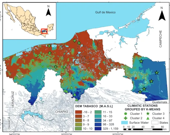
2.3 Study area

In order to apply the different imputation methods and to illustrate how the two new proposed procedures work, we have chosen the state of Tabasco, which is located in the southern region of Mexico. Tabasco is bordered by the states of Chiapas, Campeche, Quintana Roo and Yucatán (see Fig. 1), which are considered the wettest region in the country. Ta-basco extends from the coastal plain of the Gulf of Mexico to the mountain ranges of northern Chiapas. Geographically it is located between 17º 15’-18º 39’ N, and 91º 00’-94º 17’ W. It is bounded to the north by the Gulf of Mexico and the state of Campeche, to the south by the state of Chiapas, to the east by the Republic of Guatemala and to the west by the state of Veracruz (Fig. 1). Tabasco has an area of 25 267 km2_{, representing 1.3% of the Mexican territory. The}

to 36ºC. The historical yearly average rainfall in the state is of 2184.6 mm, which is the highest annual precipitation in Mexico. The highest rainfall zone is in the mountain range in the south-center part of the state, with precipitation values above 4000 mm yr–1_,

while the rest of the state has recorded precipitation values in the range of 1200 to 2500 mm yr–1_. 2.4 Climatological database

The state of Tabasco has 83 meteorological stations. However, after a careful analysis of their records, the following problems were found: i) some stations were not useful because the data was collected at different time scales (days, months and years) and ii) some stations with daily rainfall records did not have enough information. Only stations with a minimum of 30 yrs of uninterrupted rainfall information, as recommended by the World Meteorological Organi-zation (WMO, 2011) were chosen. The period from January 1, 1980 to December 31, 2012 was chosen

to conduct this investigation. Since there is not a well-established criterion of what to consider as an acceptable percentage of missing data in a time series dataset (Dong and Peng, 2013), an assumption was made to consider datasets with daily rainfall with at most 25% of missing data. This approach allowed to have a more reliable dataset, even though rainfall time series with higher percentages of missing data have been considered in other studies (Malek et al., 2010; Campozano et al., 2015; Toro-Trujillo et al., 2015). Table II shows a summary of the main features of the selected weather stations, which cover 82% of Tabasco’s municipalities (14 of 17). The information was obtained through the Climate Computing Pro-gram (Clicom) system of the National Meteorological Service (http://clicom-mex.cicese.mx). None of the weather stations selected had a complete dataset.

The standard deviation in the state varied between 12.503 and 23.230 mm day–1_{. These ranges were}

recorded in very contrasting zones: the lower range -16 - 2 11 - 15 _{Cluster 1}

Cluster 2 Surface Water 0

92º0'0''W 93º0'0''W

94º0'0''W

17º0'0''N

18º0'0''N

19º0'0''N

10 20 40 60

N N

CAMPECHE

80 km States Cluster 3 Cluster 4

DEM TABASCO [M.A.S.L] CLIMATIC STATIONS

GROUPED BY K-MEANS 16 - 33

34 - 97 98 - 328 329 - 1,159 3 - 7

8 - 8 9 - 9 10 - 10

Gulf de Mexico

CHIAPAS

Guatemala

VERACRUZ

OAXAC

A

Table II. Characteristics of the selected stations. Station Country Long (W) Lat (N) Alt (masl) MD (%) Period Max Mean Std. VC S K 27002 Centla 92.8 18.417 3 12.71 1969–2016 300 3.920 12.588 3.21 1 6.987 81.330 27004 Tenosique 91.493 17.449 14 2.22 1948–2016 190 6.303 15.400 2.443 4.106 22.623 27006 Balancán 91.275 17.638 50 2.81 1967–2016 280 4.672 12.639 2.705 5.585 52.496 27007 Cárdenas 93.619 18.001 12 15.23 1961–2016 360 5.694 17.365 3.050 6.768 75.527 27008 Cárdenas 93.376 18.001 25 12.24 1955–2016 300 5.686 16.425 2.888 6.234 61.613 27009 Comalcalco 93.22 18.247 15 19.51 1965–2016 274 4.801 15.082 3.142 6.154 56.439 2701 1 Tacotalpa 92.798 17.613 20 10.21 1950–2016 269 7.70 19.35 2.513 4.520 29.630 27015 Huimanguillo 93.942 17.837 7 24.90 1965–2016 207 6.569 16.485 2.510 4.149 23.338 27019 Jalapa 92.812 17.723 14 1.41 1970–2016 310 7.1 15 18.879 2.653 4.866 34.161 27021 Balancán 91.293 17.757 29 20.04 1969–2016 201.2 5.418 14.518 2.679 4.602 30.757 27030 Macuspana 92.605 17.757 11 0.68 1948–2016 265 6.404 16.509 2.578 4.532 29.318 27034 Paraíso 93.212 18.396 6 8.84 1949–2016 339 4.501 14.584 3.240 7.131 82.448 27036 Cunduacán 93.176 18.067 15 3.14 1970–2016 350 5.433 15.387 2.832 6.438 73.218 27037 Centro 93.879 17.854 21 2.14 1948–2016 306.4 5.680 15.312 2.696 5.258 44.671 27039 Cunduacán 93.279 17.997 23 5.22 1948–2016 268.5 5.487 15.386 2.804 5.494 46.127 27040 Balancán 91.158 17.792 44 3.28 1948–2016 273.8 4.518 12.503 2.767 5.834 55.724 27042 Tacotalpa 92.777 17.461 44 4.85 1962–2016 343.9 9.836 23.1 11 2.350 4.670 32.974 27044 Teapa 92.953 17.549 51 1.24 1960–2015 301.2 8.988 20.527 2.284 4.131 25.608 27047 Tenosique 91.427 17.472 22 24.00 1921–2015 213 5.823 15.746 2.704 4.742 30.459 27050 Centla 92.6 18.384 2 5.40 1948–2015 247 4.264 13.181 3.091 6.764 70.298 27054 Centro 92.928 17.997 24 5.86 1948–2015 340 5.386 15.283 2.838 5.776 55.439 27060 Centro 93.768 17.974 11 12.64 1972–2016 320 5.439 15.601 2.868 5.543 47.752 27061 Teapa 92.92 17.513 86 16.41 1972–2016 396.4 10.519 23.230 2.208 4.080 26.783 27070 Tacotalpa 92.75 17.381 63 1.64 1974–2016 317 8.842 20.741 2.346 4.366 28.835 27075 Cárdenas 93.566 18.1 11 10 10.23 1972–2016 334 6.297 18.346 2.914 5.887 53.335 27076 Cárdenas 93.497 18.1 11 13 24.02 1972–2016 365 6.292 19.518 3.102 7.141 74.564 27077 Cárdenas 93.625 18.066 12 13.46 1972–2016 360 5.850 18.561 3.173 5.638 48.432 27078 Cárdenas 93.499 18.021 19 6.16 1972–2016 310 4.871 15.133 3.107 6.693 73.289 27084 Nacajuca 93.018 18.166 10 6.84 1979–2016 267 4.860 14.199 2.922 5.768 49.995 Alt: altit ude given in masl; MD: percentage of missing data; Std.: standard deviation; VC: variation coefficient; S: skewness; K: kurtosis. The values of the

corresponds to weather station 27040, located in the municipality of Balancán, to the west-northwest of the state, with an annual precipitation range be-tween 1500 and 2000 mm, while the highest daily precipitation range was found in meteorological station 27061, located in the municipality of Teapa to the center-south of the state (highest rainfall area), with annual ranges above 2500 mm. The Pearson’s linear correlation coefficient between the standard deviation and the daily mean values of rainfall was 0.934. Therefore, both variables are related pos-itively, which means high values of precipitation are associated with high variability (Sokol Jurkoviç and Pasariç, 2013). This relationship allows us to obtain a variation coefficient that homogenizes the variation between all the meteorological stations. In all the weather stations, asymmetric values greater than or equal to 4.080 were obtained, therefore, the rainfall data-set have a positive biased distribution, that is, the distribution of precipitation data tends to be concentrated towards the left rather than towards the right of the mean. Finally, it can be observed that the kurtosis coefficient of the daily rainfall dis-tribution has a minimum of 22.623, implying that in all the meteorological stations there is a visible concentration of rainfall values in the central area of the distribution. As a result, all of the distributions are leptokurtic (Hood et al., 2007).

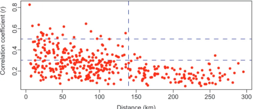
In order to provide a better perspective on the behavior of rainfall, the calculation of the correla-tions between the amount of daily rainfall with all

possible pairs of the selected weather stations was carried out. At the same time, the distances between the geographical locations of the selected stations was also computed. Figure 2 shows the correlations of the rainfall plotted against the distance, given in kilome-ters. Weather stations that are separated by distances beyond 140 km have low correlation values (lower than 0.30) and have a low degree of linear association. On the other hand, nearby weather stations have more similar rainfall behaviors than pairs of geographically distant weather stations. DeGaetano (2001) suggests that weather stations that are geographically close to each other should be grouped, because it provides an idea of the spatial structure of the variables under study. Cluster analysis is one of the most common used techniques to identify groups of homogeneous climates (DeGaetano, 2001). Given that the data satisfies the assumption of the existence of spatial correlations between the amount and the frequency of rainfall between neighboring weather stations, the choice of the latter technique was applied in our study. The above analysis is supported by the results shown in figure 2, where a negative relationship between the correlation of daily rainfall amounts and the distance between weather stations is evident.

2.5 Methodology to test the proposed methods

Taking into account that the spatial clustering of ob-servation sites is a common practice in climatology (DeGaetano, 2001; Teegavarapu, 2012), and that empirical methods use weather stations with similar

0

0.

20

.4

Correlation coef

ficient (r

)

0.

60

.8

50 100 150

Distance (km)

200 250 300

rainfall patterns (Xia et al., 1999; Teegavarapu and Chandramouli, 2005; Ramos-Calzado et al., 2008; Suhaila et al., 2008; Campozano et al., 2015), the hypothesis being tested here is that missing rainfall data in a target station can be imputed by consider-ing the daily rainfall dataset of several neighborconsider-ing weather stations. The procedure followed to evaluate our hypothesis can be summarized as follows:

1. The first step is to carry out a cluster’s analysis through the K-meansgrouping method, in order to define the geographic regions with homogeneous properties.

2. Then, it is necessary to choose a data-set without missing data in each one of the clusters.

3. After that we chose a number N of similar neigh-boring weather stations with respect to the given target station.

4. Then, for each target station and in each cluster, we applied a number of existing (previously se-lected) imputation methods.

5. The above item is complemented by applying two new proposals (not found in the literature) for the imputation of missing data.

6. Then, following a well-established criterion (mean absolute error [MAE]), we evaluated and chose the best method (optimum parameters) among the ones used in the former items.

7. Finally, an iterative algorithm was evaluated in each of the target weather stations, which applies the best imputation method (among the ones con-sidered here) in each cluster.

These steps are described in more detail in the following sections.

2.5.1 Non-hierarchical cluster analysis

Cluster analysis is one of the statistical techniques frequently used in meteorology and climatology to group stations in regions with homogeneous climates (Gong and Richman, 1995; DeGaetano, 2001). In this study, the K-mean grouping algorithm (Teegavarapu, 2014; Mohammadrezapour et al., 2018; Reddy et al., 2018;) is used to identify spatial groups of the aforementioned weather stations (see Fig. 1). This allowed for the visualization of the spatial structure of rainfall and to perform an efficient search of neigh-boring weather stations that are closest to the target

station. In order to validate the cluster’s structure, five techniques were used: 1) the elbow method, 2) the TraceW index (Milligan and Cooper, 1985), 3) the Hartigan index (Hartigan, 1975), 4) the Krzanowski index (Krzanowski and Lai, 1988), and 5) the gap statistics (Tibshirani et al., 2001). In order to evaluate the stability of the clusters, the algorithm described by Hennig (2007) was used, which was implemented using the “fpc” software package using R (Hennig, 2015). The stability evaluation of the clusters is based on the use of the Jaccard coefficient (Guha et al., 1999), while the plausible variations in the initial dataset are obtained by bootstrap resampling (Effron and Tibshirani, 1993).

2.5.2 Selection of similar neighboring stations

In all spatial interpolation schemes, the selection and amount of similar neighboring weather stations are very important factors that influence the results of the interpolations (Eischeid et al., 2000). There are many ways to select neighboring weather stations. Some are based on the correlation coefficient (Young, 1992; Eischeid et al., 1995, 2000), while in others the proximity between neighboring weather stations is represented by means of a statistical distance ap-proach (Ahrens, 2006; Ramos-Calzado et al., 2008). According to Eischeid et al. (2000) adding more than four neighboring stations does not significantly im-prove the results of the interpolation and sometimes worsen the estimates. In this work, a criterion of no more than four neighboring stations was selected as the distance between stations.

2.5.3 Evaluation of the estimation methods perfor-mance

can be achieved, is by evaluating every selected in-terpolation method in each target station. In this way it is apparent to identify the method that provides the best estimates. Usually spatial interpolation methods produce numerical errors associated with the estima-tion. Therefore, a way to compare the performance of these methods is through using measures that quan-tify the committed error. In this regard, MAE is the most natural measure to calculate the average error (Willmott and Matsuura, 2005). The aforementioned error measure is given by

MAEi = 1_n ∑nt=1|Zi(t) – Zi(t)| (11)

where n is the total number of observations, Zt (t) is

the estimated value and Zi(t) is the observed value,

related to the corresponding meteorological variable in the target station i.

2.5.4 Iterative algorithm

In this subsection we describe the iterative proce-dures used in order to establish reasonable imputed values for daily rainfall. Below we describe, first, the process to find the optimal estimation method and its parameters, and then, the algorithm for the estimation of missing data is presented.

2.5.4.1 Methodology to find the optimal estimation method

We begin by grouping the set X={x1,x2,…,xn} of

d--dimensional, n weather stations through using the K-mean method within a group of K clusters, C={ck,

k = 1,2,…,K}.. Then, for the k-th cluster in the set

C, ck a dataset is selected where there are no missing

values. The next step is to determine the number of neighboring weather stations by considering the Euclidean distance criterion:

dij= (Wik – Wjk)T (Wik – Wjk) (12)

where dij is the Euclidean distance between the i-th

and the j-th stations that belong in the cluster ck.

These are represented in the space of the variables by the vectors

Wik= and Wjk= , x1jk

x2jk xdik···

( )

x2jk xdjk···

( )

respectively. The variables we consider in this work are the longitude and the latitude in their UTM co-ordinates. Subsequently, each of the aforementioned methods shown in Table I, are evaluated. The CMA-ES optimization method was used to find optimal parameters-exponents of all weighted methods, including our proposals. For each parameter to be optimized, a search space located within the interval (10–8_{,50), was considered. In order to avoid falling}

into a local minimum, 50 iterations are performed, and the average absolute error is calculated. Finally, the optimal method for each destination station is the one that provides the absolute minimum of MAE.

2.5.4.2 Algorithm for estimating missing data

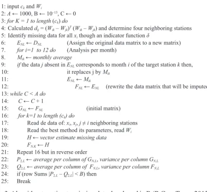
The purpose of the iterative algorithm described be-low (Fig. 3) is to establish reasonable imputed values for daily rainfall. Moreover, for the i-th target station belonging in the ck cluster, the weight-function Wi

(obtained through the methodology described in the subsection above) is required.

Firstly, the algorithm requires initial parameters. Line 1 introduces the weighting functions that are associated with the i-th stations belonging in the

ck cluster. Then, line 2 introduces a series of initial

values: A defines the maximum number of iterations to be considered, B defines the tolerance with which to work and C represents the initial value of a given counter.

Secondly, an iterative procedure is applied to each cluster from line 3 to line 21. In line 4, for each one of the xi target stations belonging in the cluster ck, the

distance from the neighboring stations is calculated by using Eq. (10). Considering each one of the dis-tances, the four neighboring stations corresponding to each one of the xi target stations are chosen. Then,

the missing data is identified by using the δ indicator function, that is, δ = 1 if the daily rainfall data in xi is

missing and δ = 0 otherwise. Line 6 assigns the origi-nal data matrix DNL, where N represents the whole set

of available data in the study for every target station, and L represents the cluster length ck to a new matrix

ENL. This is done in order to preserve the original data

and not to lose them in the imputation process. From line 7 to line 12, the missing data is replaced by the average monthly rainfall, considering the historical behavior for each one of the target stations xi. We first

each one of the target stations xi. Then, for the lacking

j in the original data ENL, corresponding to the month

i in the target station k, the missing j is replaced by the monthly average in Mik. Finally, line 12 rewrites

the data matrix that will be imputed and we name it

FNL. From line 13 to 21, the main process for

impu-tation of missing data is performed. In this part of the algorithm we start by reading the best method and its parameters (obtained in the subsection Methodology to find the optimal estimation method), the data of the

xi target stations, the data of the xj, j ≠ i neighboring

stations, as well as the different weighting functions

Wi associated with each one of the xi target stations.

Then, only the missing data are estimated, that is, the data corresponding to a value of the function

δ ≠ i. The mean value calculated in the previous stage is replaced by the values obtained when using the optimal methods. So far what has been done is a forward procedure where more than one neigh-boring station has been selected in order to estimate the missing values in one or in more than one target stations. Line 21 repeats the process started on line 16 but in an inverse manner. Therefore, a backward procedure is now being considered. It is possible that at the beginning of these processes great differences

arise, but with the passage of the iterations the process eventually stabilizes.

Finally, the stop criterion is verified in lines 22 to 25. In lines 22 and 23, two descriptive statistics are computed: the mean and the variance per column for two consecutive iterations. These are saved in matrices P2,L and Q2,L, respectively. The first row of

both matrices is composed by the arithmetic means, while in the second row the variances are found. In order to establish the stopping criterion, we evaluate whether the sum of each row of | P2,L – Q2,| is less

than 10–13_{. Therefore, there are no significant}

differ-ences between the data set with missing values and the complete data set.

In order to provide greater clarity of the iterative algorithm to estimate missing rainfall data, the flow diagram is presented in figure 4.

3. Results and discussion

3.1 Validation of the clusters’ structure

The validation and stability of the structure of the clusters is analyzed in figure 5a, which shows that clusters incorporate much information that results in high values of variance. As shown in this figure, there

1: input ck and Wi

2: A ← 1000, B ← 10–13_{, C ← 0}

3: for K = 1 to length (ck) do

4: Calculated dij= (Wik– Wjk)T (Wik– Wjk) and determine four neighboring stations

5: Identify missing data for all xithough an indicator function δ

6: ENL← DNL (Assign the original data matrix to a new matrix)

7. for i=1 to 12 do (Analysis per month) 8. Mik ← monthly average

9: if the data j absent in ENLcorresponds to month i of the target station k then,

10: it replaces j by Mik

11: ENL← Mik

12: FNL← ENL (rewrite the data matrix that will be imputed)

13: while C < A do

14: C ← C + 1

15: GNL ← FNL (initial matrix)

16: for k=1 to length (ck) do

17: Read de data of: xi, xj, j ≠ i neighboring stations

18: Read the best method its parameters, read Wi

19: H ← vector estimate missing data

20: FN,K ← H

21: Repeat 16 but in reverse order

22: P2,L ← average per column ofGN,L, variance per columnGN,L

23: Q2,L ← average per column of FN,L, variance per columnFN,L

24: if (row Sums |P2,L – Q2,L| < B) then

25: Break

is a rapid decay until a point k = 4. From this k-value on, the marginal gain drops drastically and the total sum of the squared errors within the clusters tends to change slowly. As a result, an arm-like structure with an “elbow” is observed at the point k= 4. The optimal number of clusters corresponds, precisely, to

the position of the elbow. However, the elbow method is heuristic and may or may not work always. For this reason, four different methods were also tested to compute the optimal k value; i.e., optimal number of clusters. Figure 5b shows the gap statistic method. This procedure compares the total within intra-cluster

Step 1

Step 3

Step 2 Start

Stop (see, line

25) Read cluster Ck, Weighting function Wi,

Initial values A,B and C (see, lines 1-2

Target station selection K=1 to length (ck) (see, line 3)

if k>lenght ck

Selection of neighbors (see, line 4)

Identify missing data through an indicator function δ (see, lines 5-6)

Interative process forward and backward (see, lines 13-21)

if (row Sums |P2,L – Q2,L| < B)

Replace average values ENL ← Mik (see, lines 7-12)

Yes Yes

(see, lines 22-24)

No

No

Fig. 4. Flowchart showing a summarization of the proposed method to estimate missing data. Step 1: the algorithm requires initial parameters; step 2: an iterative procedure is applied to each cluster; step 3: the stop criterion is verified.

Fig. 5. Sum of squared error against number of clusters (scree plot). (a) Gap statistic. (b) Optimal number of clusters (k = 4).

(b)

0.0 0.1 0.2 0.3 0.4 0.5

1 2 3 4 5 6 7 8 9 10

Number of clusters k

Gap statistic (k

)

Optimal number of clusters The Gap index

0.0e+00 5.0e+10 1.0e+11 1.5e+11 2.0e+11

Optimal number of clusters Elbow method

(a)

1 2 3 4 5 6 7 8 9 10

Number of clusters k

variation for different values of k with their expected values under a null reference distribution of the data. The optimal number of clusters is the value that maximizes the gap statistics. This means that the clus-tering structure is far away from the random uniform distribution of points (Tibshirani et al., 2001). This plot shows the statistics by number of clusters (k) with standard errors drawn with vertical segments and the optimal value of k marked with a vertical dashed blue line. According to this observation k = 4 is the optimal number of clusters in the data.

Table III shows the results of comparing the TraceW, Hartigan and Krzanowski indices used to find the optimal k-value. In this way, five different methods were applied to estimate the optimal num-ber of clusters. It is evident from these results that, in coincidence with the results of the elbow method, the optimal selection for k was 4.

By analyzing the stability of the structure com-posed of four clusters, the following stability values were obtained: 0.9208770, 0.9051905, 1.0000000 and 1.0000000, respectively. It can therefore be seen that the four clusters are stable. This means that there is a high probability that all of these clusters repre-sent the true structure in the data. Unlike our work, Teegavarapu (2014) carried out the estimation of missing precipitation data using optimal proximity metric-based imputation, nearest-neighbor classifica-tion and cluster-based interpolaclassifica-tion methods. In this study different cluster sizes were experimented. A total of six clusters resulted in the best performance measures.

3.2 Application and evaluation of the different im-putation methods

In order to evaluate the performance of 11 imputation methods (nine from previous studies and two new methods proposed here) of the four clusters, a data-set was selected without the presence of missing values. The comparison between the observed and imputed values was quantified using the MAE. The CMA-ES algorithm was employed in all of the weighting functions in order to find the optimal exponents.

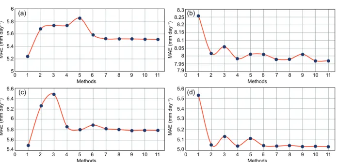
Figure 6 shoes the behavior of the MAE for each one of the 11 allocation methods evaluated. The

Table III. Values of the indices for data partitions in the state of Tabasco.

Indices Cluster number Index value

TraceW(k) 4 32255292808

H(k) 4 31.6603

KL(k) 4 10.3271

Fig. 6. Mean absolute error of the 11 deterministic imputation methods (Table I.). (a) station 27006, (b) station 27008, (c) station 27030 and (d) station 27054.

(a) (b)

(c) (d)

6

5.8

5.6

5.4

5.2

5

0 1 2 3 4 5

Methods

MAE (mm day

–1)

6.4 6.2 6 5.8 5.6 5.4 6.6

MAE (mm da

y

–1) 5.5

5.4 5.3 5.2 5.1 5.0 5.6

MAE (mm da

y

–1) 8.3 8.25 8.2 8.15

8.05

7.95 7.9 8.1

8

MAE (mm day

–1)

6 7 8 9 10 11

0 1 2 3 4 5

Methods6 7 8 9 10 11

0 1 2 3 4 5

Methods6 7 8 9 10 11

0 1 2 3 4 5

weather stations 27006, 27008, 27030 and 27054 were randomly selected to test these methods. The vertical axis represents the MAE, while the horizontal axis represents each of the methods mentioned in Table I. The new methods proposed here are identi-fied by the numbers 10 and 11 in the above-mentioned figure. In weather stations 27006 and 27030 the method that shows the minimum MAE is the normal ratio, with values of 5.236 and of 5.498 mm day–1_,

respectively. In both cases the GCIDW proposal (the one identified through the number 11 in the figure) turns out to be the second-best selection. On the other hand, in the stations 27008 and 270054, the methods 9-11 (which incorporate the altitude factor in the weighting functions) present very similar results, although method 11’ shows the minimum MAE. Therefore, the new proposals presented in this paper, show better performance than the remaining methods considered.

The values of MAE for each one of the 11 allo-cation methods evaluated is shown in Table IV, as well as the mean rank obtained by each imputation method according to the Friedmann test (Lee and Kang, 2015). In the last row, the symbol > denotes that the difference between one or more methods is statistically significant. For instance, {method1a_{} >}

{method2b_{} > {method3}bc_{, method4}c_{} indicates that}

the method 1 is significantly better than methods 2, 3 and 4. In addition, method 2 is significantly better than method 4, while method 3 does not differ signifi-cantly than methods 2, and 4 since it has common bc letters. Finally, method 3, despite not having differ-ences with method 2 is placed next to method 4 since its average ranges are greater than those obtained by method 2 and more like those obtained by method 4. The results presented in Table IV show that the calculations of MAE when applying the GCIDW method with the exception of one case (weather station 27070) were always between the three lowest values (see superscript values). Therefore, GCIDW obtained the smallest mean rank. Besides, there is a significant difference between all the methods eval-uated (significant p-value equal to 0.000). The MAE values in this work were similar to those obtained by other researchers (Deraisme et al., 2001; Suhaila et al., 2008; Qian et al., 2010; Seyyednejad et al., 2012; Serrano-Notivoli et al., 2017b). In particular, the MAE values are between 4 and 8.6 mm with an

average value close to 6 mm. Overall, performance results show that CCWM is superior compared to other methods found in the literature. Similar results were obtained by Azman et al. (2015) when they es-timated missing rainfall data in Pahang using spatial interpolation weighting methods, probably due to the fact that the used stations were in the same cluster, and it indicates a strong relationship between all the stations.

To identify which method or methods are signifi-cantly different, the Nemenyi post hoc test (Pohlert, 2014) was performed. The results indicated there are three well-defined homogeneous subgroups (see last row in Table IV.), with the proposed method (GCIDW) being statistically significantly better than the other methods compared. Therefore, GCIDW can be considered the best method to estimate missing rainfall data among the methods analyzed. In Table V the optimal method for all of the stations within each cluster is presented. The proposed imputation methods resulted optimal in 13 of the 29 stations analyzed (this represents approximately 44.83% of the weather stations). In order of priority, NR, CCWM, NRIDC and HIDW were found in 9, 4, 2 and 1 stations, respectively.

Table IV

. Friedman test with MAE values.

Station NR NR WC CCW NRIDW IDW CCWM CIDW NRIDC HIDW GNRIDW GCIDW 27002 4.58136 (1) 4.83451 (8) 4.96807 (9) 5.00777 (10) 5.15598 (1 1) 4.71 146 (7) 4.70947 (5) 4.70949 (6) 4.70946 (3) 4.70946 (3) 4.70946 (3) 27004 6.77994 (10) 6.10653 (5.5) 6.16849 (7) 7.51878 (1 1) 6.32066 (8.5) 6.09563 (4) 6.08595 (3) 6.08093 (2) 6.32066 (8.5) 6.10653 (5.5) 6.07163 (1) 27006 5.23647 (1) 5.67940 (8) 5.73487 (9) 5.73614 (10) 5.85213 (1 1) 5.58435 (7) 5.52095 (5) 5.52142 (6) 5.51980 (4) 5.51524 (3) 5.51 171 (2) 27007 6.34189 (9) 6.09271 (3.5) 6.18950 (7) 6.3021 1 (8) 6.37237 (10.5) 6.05466 (2) 6.1 1884 (5) 6.13374 (6) 6.37237 (10.5) 6.09271 (3.5) 6.04016 (1) 27008 8.25795 (1 1) 8.01815 (9) 8.05966 (10) 7.98298 (5) 8.01 101 (7.5) 8.01078 (6) 7.98051 (4) 7.97959 (3) 8.01 101 (7.5) 7.96975 (2) 7.96922 (1) 27009 6.40267 (1 1) 6.26948 (9) 6.35378 (10) 6.17743 (6) 6.26834 (7.5) 6.15654 (1.5) 6.16437 (3) 6.16509 (4) 6.26834 (7.5) 6.17518 (5) 6.15654 (1.5) 2701 1 7.01 162 (1) 7.55082 (1 1) 7.49064 (10) 7.40102 (8) 7.35470 (6) 7.47037 (9) 7.36369 (7) 7.31915 (4) 7.35466 (5) 7.28865 (3) 7.20960 (2) 27015 7.95846 (10) 7.45377 (3) 7.48694 (7) 8.20322 (1 1) 7.60466 (9) 7.45438 (4) 7.46059 (5) 7.46128 (6) 7.58492 (8) 7.44972 (1) 7.44988 (2) 27019 6.15505 (7) 6.50947 (8) 6.70646 (10) 6.63368 (9) 6.81568 (1 1) 5.87313 (4) 5.86839 (3) 5.86729 (2) 6.00239 (6) 5.93986 (5) 5.86557 (1) 27021 6.42263 (1 1) 6.25919 (9) 6.28160 (10) 6.18465 (5) 6.22970 (6.5) 6.25370 (8) 6.16238 (3) 6.17260 (4) 6.22970 (6.5) 6.15686 (2) 6.14868 (1) 27030 5.49057 (1) 6.24662 (10) 6.46559 (1 1) 5.84851 (8) 5.78529 (5) 5.88026 (9) 5.80920 (7) 5.79325 (6) 5.77303 (2.5) 5.77951 (4) 5.77303 (2.5) 27034 4.79522 (6) 4.78950 (5) 4.85699 (7) 5.10866 (1 1) 4.99321 (10) 4.78209 (4) 4.92023 (9) 4.90330 (8) 4.72684 (1.5) 4.75235 (3) 4.72684 (1.5) 27036 6.33703 (1 1) 5.92331 (4) 5.94339 (5) 5.99212 (8) 6.1 1030 (9.5) 5.92106 (1.5) 5.99035 (7) 5.98986 (6) 6.1 1030 (9.5) 5.92271 (3) 5.92106 (1.5) 27037 6.13804 (9) 5.32788 (7) 5.68747 (8) 6.14029 (10) 6.17238 (1 1) 5.26160 (4) 5.32653 (6) 5.32557 (5) 5.25829 (3) 5.25275 (2) 5.25078 (1) 27039 6.19450 (1) 6.29664 (5) 6.34208 (6) 6.73254 (1 1) 6.42501 (9.5) 6.29204 (3) 6.38629 (8) 6.38101 (7) 6.42501 (9.5) 6.29424 (4) 6.28707 (2) 27040 5.08625 (1) 5.35654 (8) 5.38551 (9) 5.51924 (1 1) 5.48610 (10) 5.35309 (7) 5.21965 (3) 5.22774 (5) 5.32263 (6) 5.22181 (4) 5.21821 (2) 27042 6.98728 (1 1) 6.43215 (9) 6.67242 (10) 6.29520 (8) 6.28697 (7) 6.26032 (3) 6.26488 (4) 6.27846 (5) 6.28578 (6) 6.25526 (2) 6.25303 (1) 27044 5.42147 (1 1) 4.06819 (8) 4.82861 (10) 4.24727 (9) 4.03553 (3) 4.04552 (6) 4.06398 (7) 4.02684 (1) 4.03553 (3) 4.03769 (5) 4.03553 (3) 27047 7.93838 (8) 7.64081 (6.5) 7.57245 (5) 8.55550 (1 1) 7.52067 (2.5) 7.52067 (2.5) 8.40706 (10) 8.31264 (9) 7.52067 (2.5) 7.64081 (6.5) 7.52067 (2.5) 27050 4.23082 (1) 4.34225 (10) 4.34457 (1 1) 4.27002 (6) 4.27301 (7) 4.34123 (9) 4.2691 1 (5) 4.27618 (8) 4.25479 (4) 4.24716 (3) 4.24713 (2) 27054 5.52828 (1 1) 5.05456 (8) 5.13519 (10) 5.04497 (5) 5.1 141 1 (9) 5.04601 (6) 5.04123 (4) 5.04756 (7) 5.03795 (2) 5.03950 (3) 5.03697 (1) 27060 5.82079 (1 1) 5.10067 (7) 5.41674 (8) 5.07405 (6) 5.75415 (9.5) 5.03720 (4) 5.02729 (3) 5.02691 (2) 5.75415 (9.5) 5.07345 (5) 5.02561 (1) 27061 6.23225 (1 1) 4.50914 (9) 5.69481 (10) 4.25795 (8) 4.23449 (6) 4.22712 (4) 4.23210 (5) 4.23722 (7) 4.22547 (2) 4.22699 (3) 4.22537 (1) 27070 7.13218 (1 1) 6.82955 (9) 7.07248 (10) 6.70350 (8) 6.61 122 (2.5) 6.65384 (7) 6.61371 (4) 6.60310 (1) 6.61 122 (2.5) 6.62048 (5.5) 6.62048 (5.5) 27075 8.41981 (1 1) 7.65928 (6) 7.75188 (7) 7.89028 (10) 7.86985 (9) 7.62878 (3) 7.65905 (5) 7.65235 (4) 7.77776 (8) 7.61372 (2) 7.61337 (1) 27076 7.54194 (1 1) 7.17438 (3.5) 7.26591 (5) 7.34792 (8) 7.41980 (9.5) 7.16741 (1.5) 7.29444 (7) 7.28799 (6) 7.41980 (9.5) 7.17438 (3.5) 7.16741 (1.5) 27077 8.33861 (1) 8.52334 (6.5) 8.54961 (8) 8.64898 (1 1) 8.57721 (9.5) 8.40869 (3) 8.42298 (5) 8.41384 (4) 8.57721 (9.5) 8.52334 (6.5) 8.33910 (2) 27078 6.68910 (1) 6.88344 (7) 7.02124 (9) 6.9431 1 (8) 7.21660 (1 1) 6.84699 (2.5) 6.85039 (5) 6.85037 (4) 7.17412 (10) 6.87759 (6) 6.84699 (2.5) 27084 5.18968 (1 1) 4.89849 (4.5) 4.98309 (8) 4.93012 (7) 5.12807 (9.5) 4.88829 (3) 4.92240 (6) 4.87912 (2) 5.12807 (9.5) 4.89849 (4.5) 4.81314 (1) Ranking 7.28 7.14 8.48 8.52 8.22 4.67 5.28 4.83 6.09 3.74 1.76 {GCIDW a ,GNRIDW a }>{CCWM b ,NRIDC b ,CIDW b }>{HIDW bc ,NR WC bc ,NR bc ,IDW c ,CCW c ,NRIDW c } Lower ranking implies that the method is better . Equal letters a, b, c, d mean that the methods belong to the same homogenous subgroup. Dif ferent superscripts

imply that the methods belong to dif

ferent homogeneous subgroups.

Superscript represents the range obtained for each method by meteorological

station.

Finally, the inclusion of the factor that mea-sures the difference in altitude between the target station and the neighboring stations, as well as the optimization of the parameters corresponding to the correlation exponents, p, distance, q and altitude, s, contributed significantly to the computation of better estimates of missing rainfall values.

4. Conclusions

In this work we have proposed two new general-ized weighting methods and a methodology to fill missing data through using the optimal method and parameters. In these procedures we have incorporat-ed the altitude difference between the target station

and the neighboring stations, as a new variable. The performance of each method was quantified by the MAE. For all of the weight-functions required to find optimal exponents, the metaheuristic adaptation of the covariance matrix (CMA-ES) was employed. The results of this process show that the proposed meth-ods are optimal at 44.83%, followed by the classical normal ratio method with approximately 31%.

The weather stations of the state of Tabasco were clustered through the K-mean procedure, which is based on the Euclidean distance. In our analysis, UTM coordinates were used in order to locate the weather stations representing each east coordinate as a value on the x-axis and each north coordinate as a value on the y-axis. In order to validate the amount

Table V. Selection of the optimal method for all stations within each cluster. Membership Station Optimal

method MAE p q s

Cluster 1

27007 11 6.040 6.33 6.91·10–9 _0.214

27008 11 7.969 2.23 1.24 5.97·10–9

27015 10 7.45 2.62·10–9 _2.18·10–1

-27037 11 5.251 3.95 1.18·10–9 _2.89

27039 1 6.194 - -

-27060 11 5.026 6.4 3.85·10–9 _0.386

27075 11 7.613 2.41 1.72·10–9 _1.27

27076 5 7.167 2.86 -

-27077 1 8.339 - -

-27078 1 6.689 - -

-Cluster 2

27002 1 4.581 - -

-27009 5 6.157 8.323 -

-27034 9 4.727 1.96 3.36

-27036 5 5.921 1.784 -

-27050 1 4.231 - -

-27054 11 5.037 1.116 3.61 1.098

27084 11 4.813 18.283 5.96·10–9 _6.137

Cluster 3

27004 11 6.072 30.5 10.776 0.278

27006 1 5.236 - -

-27021 11 6.149 3.99 1.263 10–4

27040 1 5.086 - -

-27047 5 7.521 10–4 _-

-Cluster 4

27011 1 7.012 - - 9.42·10–9

27019 11 5.866 14.5 3.17 9.42

27030 1 5.491 - -

-27042 11 6.253 3.8 1.16 2.56·10–9

27044 8 4.027 9.94·10–9 _-

-27061 11 4.225 7.93 4.67·10–10 _0.529

of clusters, five methods were employed: (1) elbow method, (2) gap statistics, (3) TraceW index, (4) Hartigan index, and (5) Krzanowski and Lai index. The first two are graphic methods and in all cases

the same results were computed. The study on the validity of the optimal number of clusters ends up with the stability study by using an algorithm based on the bootstrap method. All of the stability indices

Table VI. Performance statistics for the original and imputed series.

Membership Station Series Mean STD VC S K

Cluster 1

27007 Original_imputed 5.694_5.560 17.365_16.758 3.050_3.014 6.768_6.811 75.527_76.970

27008 Original_imputed 5.686_5.617 16.425_16.097 2.888_2.866 6.234_6.203 61.613_61.018

27015 Original_imputed 6.569_6.264 16.485_15.686 2.510_2.504 4.149_4.354 23.338_25.960

27037 Original_imputed 5.680_5.650 15.312_15.306 2.696_2.709 5.258_5.251 44.671_44.322

27039 Original_imputed 5.487_5.450 15.386_15.252 2.804_2.799 5.494_5.527 46.127_46.516

27060 Original_imputed 5.439_5.397 15.601_15.361 2.868_2.846 5.543_5.526 47.752_47.220

27075 Original_imputed 6.297_6.231 18.346_18.073 2.914_2.901 5.887_5.852 53.335_52.796

27076 Original_imputed 6.292_6.133 19.518_18.257 3.102_2.977 7.141_7.131 74.564_77.017

27077 Original_imputed 5.850_5.798 18.561_17.846 3.173_3.078 5.638_5.697 48.432_50.146

27078 Original_imputed 4.871_4.859 15.133_14.838 3.107_3.054 6.693_6.714 73.289_74.634

Cluster 2

27002 Original_imputed 3.920_3.947 12.588_12.132 3.211_3.074 6.987_6.985 81.330_83.146

27009 Original_imputed 4.801_4.713 15.082_14.562 3.142_3.089 6.154_6.586 56.439_67.426

27034 Original_imputed 4.501_4.534 14.584_14.324 3.240_3.159 7.131_7.049 82.448_81.585

27036 Original_imputed 5.433_5.440 15.387_15.284 2.832_2.809 6.438_6.411 73.218_73.007

27050 Original_imputed 4.264_4.339 13.181_13.022 3.091_3.001 6.764_6.697 70.298_69.929

27054 Original_imputed 5.386_5.409 15.283_15.124 2.838_2.796 5.776_5.759 55.439_55.272

ensured that the four clusters obtained represent the true structure of the dataset.

Choosing the optimal procedure for the analysis of missing data is a huge task, since a particular method can provide optimal estimates only for certain situations. In this regard, when analyzing missing data, our research shows that it is necessary to apply more than one alternative to evaluate each case and decide which method should be the optimal. In terms of performance, one of our proposals, specifically the GCIDW, yields better results in estimating missing rainfall data than those commonly used in litera-ture. The numerical and graphical results computed by comparing the statistics of the original rainfall series with the imputed series show that there are no significant differences between the two series.

Therefore, complete daily rainfall databases were obtained without significant statistical differences for the analyzed period (1980-2012). This procedure can be used in future research such as, for instance, multifractal rainfall analysis. The new methods pro-posed in this work represent new tools not only for the treatment of rainfall missing data in the specific stations analyzed, but they can be safely applied to any other set of weather stations anywhere.

Acknowledgments

The authors thank the two anonymous reviewers and associate editor for their comments, objective and constructive criticism, which helped to improve the quality of the paper. In addition, J.L.M.M thanks the

Table VI. Performance statistics for the original and imputed series.

Membership Station Series Mean STD VC S K

Cluster 3

27004 Original_imputed 6.303_6.342 15.400_15.443 2.443_2.435 4.106_4.091 22.623_22.386

27006 Original_imputed 4.672_4.657 12.639_12.521 2.705_2.689 5.585_5.602 52.496_53.069

27021 Original_imputed 5.418_5.243 14.518_13.645 2.679_2.603 4.602_4.755 30.757_33.368

27040 Original_imputed 4.518_4.519 12.503_12.420 2.767_2.748 5.834_5.802 55.724_55.484

27047 Original_imputed 5.823_5.756 15.746_14.634 2.704_2.542 4.742_4.784 30.459_32.302

Cluster 4

27011 Original_imputed 7.70_7.79 19.35_18.89 2.513_2.425 4.52_4.47 29.63_29.56

27019 Original_imputed 7.115_7.173 18.879_18.962 2.653_2.643 4.866_4.855 34.161_33.868

27030 Original_imputed 6.404_6.423 16.509_16.488 2.578_2.567 4.532_4.523 29.318_29.263

27042 Original_imputed 9.836_9.638 23.111_22.877 2.350_2.374 4.670_4.719 32.974_33.577

27044 Original_imputed 8.988_8.985 20.527_20.488 2.284_2.280 4.131_4.126 25.608_25.554

27061 Original_imputed 10.519_10.229 23.230_23.011 2.208_2.249 4.080_4.199 26.783_27.749

Consejo Nacional de Ciencia y Tecnología (CONA-CYT) of Mexico for financial support throughout the Ph.D. program on water sciences and technology, grant No. 003497. F.A.H-R; and J.H.H acknowl-edge the Departamento de Ingeniería Civil and the Departamento de Ingeniería Geomática e Hidráulica of the Universidad de Guanajuato for the financial support for this project. And I.S.-D acknowledges the Departamento de Matemáticas Puras y Aplicadas of the Centro de Investigación en Matemáticas, A.C.

References

Ahrens B (2006). Distance in spatial interpolation of daily rain gauge data. Hydrology and Earth System Sciences Discussions10:197-208.

DOI: 10.5194/hess-10-197-2006

Al-Ahmadi K, al-Ahmadi SJA. (2013). Rainfall-altitude relationship in Saudi Arabia. Advances in Meteorology 2013:363029. DOI: 10.1155/2013/363029

Arsenault R, Poulin A, Coté P, Brissette F. (2013). Com-parison of stochastic optimization algorithms in hy-drological model calibration. Journal of Hydrologic Engineering19:1374-1384.

DOI: 10.1061/(ASCE )HE.1943-5584.0000938 Azman MA-z, Zakaria R, Ahmad Radi NF. (2015).

Estima-tion of missing rainfall data in Pahang using modified spatial interpolation weighting methods. AIP Confer-ence Proceedings 1643, 65. DOI:10.1063/1.4907426 Bajjali W. (2018). ArcGIS for environmental and water

issues. Springer, 353 pp.

DOI: 10.1016/j.jhydrol.2006.09.024

Boke AS. (2017). Comparative evaluation of spatial interpolation methods for estimation of missing me-teorological variables over Ethiopia. Journal of Water Resource and Protection9:945.

DOI: 10.4236 / jwarp.2017.98063

Campozano L, Sánchez E, Avilés A, Samaniego E. (2015). Evaluation of infilling methods for time series of daily precipitation and temperature: The case of the Ecua-dorian Andes. Maskana5:99-115.

DOI: 10.18537/mskn.05.01.07

Chang CL, Lo SL, Yu SL. (2005). Applying fuzzy theory and genetic algorithm to interpolate precipitation.

Journal of Hydrology314:92-104. DOI: 10.1016/j.jhydrol.2005.03.034

Chang CL, Lo S-L, Yu S-L. (2006). The parameter op-timization in the inverse distance method by genetic

algorithm for estimating precipitation. Environmental Monitoring and Assessment117:145-155.

DOI: 10.1007/s10661-006-8498-0

Chen F-W, Liu C-W. (2012). Estimation of the spatial rainfall distribution using inverse distance weighting (IDW) in the middle of Taiwan. Paddy and Water Environment10:209-222.

DOI: 10.1007/s10333-012-0319-1

De Silva RP, Dayawansa NDK, Ratnasiri MD. (2007). A comparison of methods used in estimating missing rainfall data. Journal of Agricultural Sciences 3. DOI: 10.4038/jas.v3i2.8107

DeGaetano AT. (2001). Spatial grouping of United States climate stations using a hybrid clustering approach.

International Journal of Climatology21:791-807. DOI: 10.1002/joc.645

Deraisme J, Humbert J, Drogue G, Freslon N. (2001). Geo-statistical interpolation of rainfall in mountainous ar-eas. In: geoENV III — Geostatistics for environmental applications. Quantitative Geology and Geostatistics, vol 11. Springer, Dordrech,

Deraisme J, Humbert J, Drogue G, Freslon N. (2001). Geostatistical interpolation of rainfall in mountainous areas. In: GeoENV III—Geostatistics for Environmen-tal Applications (pp. 57-66): Springer.

DOI: 10.1007/978-94-010-0810-5_5

Dong Y, Peng C-YJ. (2013). Principled missing data meth-ods for researchers. Springer Plus2:222.

DOI: 10.1186/2193-1801-2-222

Du K-L, Swamy MNS. (2016). Particle swarm optimization. In: Search and optimization by metaheuristics. Springer, 153-173. DOI: 10.1007/978-3-319-41192-7_9

Effron B, Tibshirani RJ. (1993). An introduction to the bootstrap. Springer, 436 pp. (Chapman & Hall/CRC Monographs on Statistics and Applied Probability). Eischeid JK, Bruce Baker C, Karl TR, Diaz HF. (1995).

The quality control of long-term climatological data using objective data analysis. Journal of Applied Me-teorology34:2787-2795.

DOI:10.1175/1520-0450(1995)034<2787:TQCO LT>2.0.CO;2

Eischeid JK, Pasteris PA, Diaz HF, Plantico MS, Lott NJ. (2000). Creating a serially complete, national daily time series of temperature and precipitation for the western United States. Journal of Applied Meteorology 39, 1580-1591.