Inferential misconceptions and
replication crisis
ABSTRACT
Misinterpretations of the p value and the introduction of bias through arbitrary analytical choices have been discussed in the literature for decades. Nonetheless, they seem to have persisted in empirical research, and criticisms of p value misuses have increased in the recent past due to the non-replicability of many studies. Unfortunately, the critical concerns that have been raised in the literature are scattered over many disciplines, often linguistically confusing, and differing in their main reasons for criticisms. Misuses and misinterpretations of the p value are currently intensely discussed under the label “replication crisis” in many academic disciplines and journals, ranging from specialised scientific journals to Nature and Science. In a drastic response to the crisis, the editors of the journal Basic and Applied Social Psychology even decided to ban the use of p values from future publications at the beginning of 2015, a fact that has added fuel to the discussions in the relevant scientific forums. Finally, in March 2016, the American Statistical Association released a brief statement on p values that explicitly addressed misuses and misinterpretations. In this context, we systematise the most serious flaws related to the p value and discuss suggestions of how to prevent mistakes and reduce the rate of false discoveries in the future.
Key words: Bayes’ Theorem; error probability; hypothesis testing; p-hacking; p values, replication crisis, statistical significance
Norbert Hirschauer (1), Oliver Musshoff (2), Sven Gruener (1), Ulrich Frey (3), Insa Theesfeld (1), Peter Wagner (1)
(1) Martin Luther University Halle-Wittenberg, Institute of Agricultural and Nutritional Sciences, Halle (Saale), Germany
(2) Georg-August-University Goettingen, Department for Agricultural Economics and Rural Development, Goettingen, Germany (3) German Aerospace Center (DLR), Stuttgart, Germany
CORRESPONDING AUTHOR:Norbert Hirschauer, Martin Luther University Halle-Wittenberg, Institute of Agricultural and Nutritional Sciences, Halle (Saale), Germany - [email protected] - phone: +49 (0)3455522362 - fax: +49 (0)3455527110
DOI: 10.2427/12066
Accepted on October 7,2016
INTRODUCTION
The reliability of statistically identified relationships is generally evaluated on the basis of p values. Using p value thresholds is commonly seen as an adequate approach to limit type I errors. A type I error is the (wrong) conclusion that there is an effect where in fact there is
none. In statistical analysis, the established convention is to refer to findings with p values up to 0.05 as “statistically significant” results. Frequently the p value is also referred to as “(type I) error probability". Both terms are highly problematic as they invite serious misunderstandings.
with “large/strong,” or “important". Second, a logical fallacy may be caused if results that are not statistically significant are described with wordings that ignore the “law of the excluded middle” (lat. tertium non datur) and suggest a confirmation of the null hypothesis (no effect). Third, researchers who are keen on obtaining low p values may introduce biases because they selectively search for and use analytical approaches that “work” in terms of producing statistical significance (p-hacking). Fourth, the term “error probability” may semantically suggest the interpretation that the p value indicates the false discovery rate, i.e., the probability of making an error when rejecting the null hypothesis1. This is not correct. The p value is nothing more than the conditional probability to observe an effect (or even a larger effect) in a random sample if, as a thought experiment, we assume that the null hypothesis (no effect) is true. Per definition, the p value can thus not convey information on the probability of the null hypothesis and therefore the false discovery rate.
Problems related to the interpretation and use of p values have been discussed in the scientific literature for decades, in particular within the field of medicine
and psychology2. Nonetheless, errors seem to
have persisted in empirical research, and criticisms of inappropriate interpretations and manipulations of the p value have increased in the recent past3 – mainly due to the non-replicability of many studies (replication crisis). In a drastic response to the crisis, the editors of the journal Basic and Applied Social Psychology even decided to ban the use of p values from future publications at the beginning of 2015 (Trafimow and Marks [19]), a fact that has added fuel to the discussions in the relevant scientific forums. In early March 2016, the visibility of the discussion appears to have reached a preliminary climax with the American Statistical Association releasing a statement on the proper use and interpretation of the p value (Wasserstein and Lazar [20]). Unfortunately, the critical concerns that have been raised in the literature are not only scattered over many academic disciplines but often are linguistically confusing and differing in
their main reasons for criticisms. It also seems that, so far, the perception of and participation in the scientific debate regarding the p value problem has remained rather limited in some disciplines such as economics4. Failures to sufficiently address the issue in academic teaching in general have been lamented long ago, however5. Against this background, our methodological comment systematises and specifies the most serious flaws and discusses suggestions of how best to prevent misinterpretations and misuses in the future and, in particular, of how to reduce the rate of false discoveries.
Problem 1: Semantic equation of “significant” with “large/strong”
Generally, the term “statistically significant” is attached to small p values – a practice that gives rise to a serious misinterpretation if “significant” is interpreted in a colloquial way and associated with a “large/strong” or an “important” effect. The risk of this misinterpretation is especially high when authors drop the adjective “statistically” and describe study results simply as “significant” or “not significant". What often follows is a verbalisation that compares a significant result with a not significant result by using the adjective “stronger” or “more”. This is not correct. A statement that a variable X has a “significant” effect on a variable Y provides no information whatsoever on the size of the effect. It only means that we have a low probability of finding the observed (or even a larger) effect by chance in a random sample if there is no effect in the parent population. Since the flawed equation of “significant” with “large/strong” is widespread and almost invited from a linguistic point of view, we briefly illustrate the issue with two stylised examples.
Example 1: We look at two pig-fattening groups. One hundred pigs are fattened with the conventional feed (CF) while another 100 pigs are fattened with an enhanced feed (EF). The pigs in fattening group CF show an average daily weight gain of 700 g. The pigs in
1 Following Colquhoun [1] and Motulsky [2, 3] and many others, we refer to the “false discovery rate,” which has been introduced (as an instrument to
multiple testing) by Benjamini and Hochberg [4], to denote the a posteriori probability of making an error when rejecting the null hypothesis. For an overview of the notional links with the problem of multiple hypothesis testing, see Efron [5] and Storey [6].
2 Selected examples are Sedlmeier and Gigerenzer [7], Kirk [8], Sterne and Smith [9], Ioannidis [10], and Colquhoun [1]. Besides the didactically
well-designed and comprehensible textbooks of Cumming [11], Kline [12], and Motulsky [3], it is especially worth pointing to Nickerson [13]. In an extensive and systematic review titled “Null hypothesis significance testing: A review of an old and continuing controversy,” Nickerson provides comprehensive insights into the p value issue.
3 Under the heading “A Dirty Dozen” Goodman [14] describes the most widespread semantic and logical misinterpretations of the p value. Colquhoun [1]
fattening group EF show an average daily weight gain of 702 g. The standard deviation amounts to 2 g in both groups. The fattening-enhancing effect is obviously small and of little economic importance. According to conventional statistical wording, we would say, however, that the effect is highly (statistically) significant (p = 10−12; one-sided t-test).
Example 2: While fattening group CF still has an average daily weight gain of 700 g, group EF has now an average daily weight gain of 750 g. Both groups count only 40 pigs now and the standard deviation is 200 g in both groups. The size of the fattening-enhancing effect of feed EF is higher by a factor 25 in example 2 compared to example 1. While the effect in example 2 is large and economically relevant, it is not statistically significant (p = 0.135; one-sided t-test). In other words, given the usually required significance level of 0.05, a researcher would not dare to exclude that the effect observed in the sample is a chance effect (random sampling error).
Large samples are rightfully considered to increase the reliability of statistically identified relationships. It should be noted, however, that the flawed equation of (statistical) “significance” and “importance” may produce especially severe and frequent misinterpretations in the analysis of very large samples. This is because the p value decreases ceteris paribus (i.e., holding both variability and effect size constant) with increasing sample size. In example 2, for instance, the p value would ceteris paribus fall to 0.05 if the size of each fattening group grew to 88. While the size of the effect in this example was large, we are facing a general mechanism. That is, any effect, no matter how small or meaningless it may be, will eventually show statistical significance if we increase sample size. A completely meaningless mini-effect will never become relevant, however, no matter how much sample size is increased6.
Problem 2: False interpretations of p values above the
significance level
In the course of a regression Y = f(X1, X2, …, Xn), it is common practice to test the coefficients 1, 2, …, n of the regressors X1, X2, …, Xn for significance. With a view to our pig-fattening example, we could think of Y as the daily weight gain and of X1 as a dummy that specifies the fattening group CF as opposed to fattening group EF. In this case, the p value of the coefficient 1 would express the probability that the observed difference in daily weight gains (or an even larger difference) were realised as a random event if the null hypothesis (no difference) were true.
The decision to reject the null hypothesis (no effect) is usually based on the commonly accepted criterion whether the significance threshold of p = 0.05 is met7. In following this practice, the question arises of how to interpret p values above 0.05 (not statistically significant results). Here again, errors in reasoning are invited by misleading but frequently used wordings. A correct and linguistically unambiguous formulation for a result with a p value above the usual significance level of 0.05 reads as follows:
The null hypothesis that the regressor X1 has no effect on Y cannot be rejected with the usually required significance level of 0.05.
This accurate though somewhat cumbersome wording complies with the “law of the excluded middle” (lat. tertium non datur), according to which a statement has to be formulated such that either the statement itself holds or its negation8. The statement “Jack is either blond or not blond” is a correct statement. However, the statement “Jack is either blond or black-haired” (or analogously: “If Jack is not blond, then he is black-haired”) is a violation of the law of the excluded middle. In this case, a false dichotomy is established, a dichotomy which disregards that there might be a third possibility, namely that Jack’s hair colour
4 To our knowledge, two important exceptions in the past are McCloskey and Ziliak [21] and Ziliak and McCloskey [22], who especially criticised the
disregard of effect size (“sizeless economics”). With the 2015 Special Issue of the Journal of Management on “Bayesian Probability and Statistics in Management Research,” parts of the present discussion on the p value were finally covered by a prominent economic journal.
5 Kline ([12] p.10), referring to Hubbard and Armstrong [23], speaks of a “major educational failure". Back in the early 2000s, Sellke et al. ([24] p.71)
diagnosed in The American Statistician a severe problem in the academic teaching of statistics: “The standard approach in teaching–of stressing the formal definition of a p value while warning against its misinterpretation–has simply been an abysmal failure". Dunn et al. [25] provide evidence that the problems in teaching are not limited to academics. According to the authors, teachers at school level have shortcomings defining even simple statistical terms.
6 The flawed equation of “significance” and “importance” appears to be not only widespread but also persistent. Analysing all 182 econometric papers
in the American Economic Review in the 1980s, McCloskey and Ziliak ([21] p.106-107) found that “70 percent of the empirical papers in the "American Economic Review" papers did not distinguish statistical significance from economic, policy, or scientific significance. […] 59 percent used the word ‘significance’ in ambiguous ways, at one point meaning ‘statistically significantly different from the null’, at another ‘practically important’ or ‘greatly changing our scientific opinions’, with no distinction". Nuzzo ([18] p.151) calls this “muddled thinking“ and Motulsky ([2] p.204) states: “The word ‘significant’ is often misunderstood. The problem is that ‘significant’ has two distinct meanings in science […]. One meaning is that a p value is less than a preset threshold (usually 0.05). The other meaning of ‘significant’ is that an effect is large enough to have a substantial […] impact. These two meanings are completely different, but are often confused".
7 In this section, we limit our discussion to the logical fallacy that lurks when interpreting p values above the significance level. In this discussion, we follow
is neither blond nor black but of a different colour. A similar false dichotomy lurks when interpreting p values above 0.05, especially if errors of reasoning are invited by lax linguistic formulations such as the following:
The hypothesis that X1 has an effect on Y cannot be accepted at the significance level of 0.05.
The hypothesis that X1 has a statistically significant effect on Y must be rejected.
While these formulations might be considered as being still acceptable by some researcher, they are definitely at the origin of wordings that become more and more misleading because they inappropriately shorten the statement or inadvertently swap the sequence of words – not dissimilar to the game of Chinese whispers. The resulting wordings often read as follows:
The effect of X1 on Y is not statistically significant. [n-s-s]
The effect of X1 on Y is statistically not significant. [s-n-s]
The effect of X1 on Y is not significant. [n-s] The effect of X1 on Y is nonsignificant. [n-s]
From the last formulation [n-s], which already insinuates that a study has found an indication of little to no effect, the false dichotomy is only a step further; and when the adjective “significant” is dropped or replaced, the definitely false conclusion follows immediately:
Our results indicate that there is no (relevant) effect of X1 on Y. [n]
With p > 0.05, it would have been correct to state that one cannot reject the hypothesis that X1 has no effect on Y using the usual significance level. The conclusion that one has found an indication of no (relevant) effect would be wrong, however. The false conclusion is triggered by wordings which suggest the false dichotomy that one can either reject the null hypothesis (if p ≤ 0.05) or accept the null hypothesis (if p > 0.05). The only thing that would have been correct to say in the case of p > 0.05 is that we simply cannot conclude whether X1 has an effect on Y or not9. Let us look back to our exemplary study that finds, with reference to a p value of 0.135, that “the new pig feed has no (statistically) significant effect on the daily weight gains". This result can by no means be interpreted as an indication that there is little
or no effect. The only allowable interpretation is that we have not yet found conclusive evidence and that we need further research. The false dichotomy fallacy in the interpretation of p values is also found in wordings in which it is not apparent at first sight. Results that are not statistically significant are occasionally commented on, for example, as being contrary to theoretical expectations or earlier findings that suggested that there is an effect. This is an inadmissible conclusion that could be only drawn if we could interpret p > 0.05 as a confirmation of the null hypothesis (no effect). This is not correct, however10.
Problem 3: p-hacking
To understand the p-hacking problem, we need to have in mind that the p value is calculated from, and only from, the data of a random sample. Low p values can hence indicate two very different cases: first, the effect observed in the data is so extreme that it is very improbable that it would be observed in a random sample drawn from a population in which there is no effect. Second, the effect is observed in the data because the sample is biased. Which of the two cases applies is not revealed by the p value. Instead, we have to impartially scrutinise both the data material and the analytical procedures. A precise interpretation of p ≤ 0.05 would thus be the following conditional statement: If both the data and the analysis are unbiased, then the hypothesis “X1 has an effect on Y” can be accepted with the usually required significance level of 0.05.
For illustration sake, let us look at an extreme case of a biased sample. If, in our example 2, we considered, for some obscure and illegitimate reason, only the upper 75% of the pigs in fattening group EF, we would find an even larger difference in average daily weight gains compared to group CF. We would also find a smaller p value. If we focused exclusively on the computed p value, we might thus be tempted to conclude that the “enhanced” feed EF causes a strong and statistically significant increase of daily weight gains. It is obvious, however, that such a conclusion would be completely flawed. Of course, one only runs the risk to succumb to such a flaw if one forgets that the p value merely indicates how (im)probable it is that
8 The reasoning associated with “the law of the excluded middle” is not a new one. It can be traced to the Greek philosopher Aristotle (384-322 BC) who
has already described this “law” in his famous work Metaphysics IV 7 (for a translation see, e.g., Lawson-Tancred [26]).
9 In this context McCloskey and Ziliak ([21] p.102) write: “Failing to reject [the null hypothesis] does not of course imply that the null is therefore true". 10 Goodman ([14] p.137) explicitly takes up this problem and describes the assumption that “studies with p values on opposite sides of 0.05 are
conflicting” as a central misunderstanding in the interpretation of the p value. Greenland et al. ([27] p.4) make the following succinct statement: “A large P-value only suggests that the data are not unusual if all the assumptions used to compute the P-value (including the test hypothesis) were correct. […] P > 0.05 only means that a discrepancy from the hypothesis prediction (e.g., no difference between treatment groups) would be as large or larger than that observed more than 5% of the time if only chance were creating the discrepancy".
11 Ioannidis ([10] p.0696) takes up this problem under the provocative heading “Why Most Published Research Findings are False” and considers biases as
the observed (or even a larger) effect would be randomly realised in a sample if in fact it were zero. Admittedly, there is a non-random inter-group difference after the data manipulation; yet this difference – no matter what the computed p value amounts to – fails to say anything meaningful about the effect of the “enhanced” feed EF.
At first sight, the issue may seem trivial since the sample above was blatantly manipulated and distorted. However, there is ample scope in the process of research to explore and selectively use analytical alternatives that, while producing serious biases and finally leading to false discoveries, “work” in terms of producing low p values11. The term p-hacking has been coined to describe the behaviour of researchers who, driven by their self-interested desire to find statistically significant (and presumably publishable) results, make such selective choices12. Since the choices between analytical alternatives rarely represent unambiguous decisions, it is difficult to find out from the outside whether a researcher’s choice is scientifically sound or the result of arbitrary p-hacking. A diligently balanced and substantiated selection of an analytical approach from the set of available alternatives is not p-hacking. However, we face p-hacking that leads to an increased risk of a false discovery if researchers selectively hunt for and report only those analytical variants that “work” and produce lower p values than other variants13.
In brief, we may state that it is difficult to see whether a certain approach is appropriate (i.e., reduces flaws) or whether it is inappropriate (i.e., produces flaws). It is reasonable, for example, to eliminate a data set that contains obviously absurd outlier values such as a yield of 87 t of wheat per hectare from the analysis. In some cases, it may also be justifiable to correct such data using common sense (in our example changing to 8.7 t of wheat per hectare). Of course, both manipulations would have to be clearly reported. Researchers are engaging in p-hacking, however, when they selectively manipulate data – for example by removing the lowest and the highest 10% of observations (or all observations outside the range of plus/minus two standard deviations from the mean) – to check whether they can thus obtain low p values. The fact
that popular statistical software packages offer convenient routines to “improve” significance exacerbates the problem14. At least for beginners, such routines may foster the erroneous belief that selectively exploring different data sets until one finds one that produces “significance” is an acceptable standard procedure.
The fact that it is so easy to check out a variety of different data sets and methods with the usual statistical software packages has increased the scope of p-hacking15. Unfortunately, this development has not been paralleled by an increasing awareness of its fatal consequences. Rather, all too many researchers have adopted the self-serving belief that the selective choice of an analytical alternative that produces the desired “statistical significance” is justifiable. In other words, many researchers do not even consider significance-pursuing behaviour as p-hacking that produces biases and increases the risk of false discoveries16. What makes things worse is that some researchers, when in a reviewer position, even encourage or request such exploratory behaviours. However, things are changing. Due to the non-replicability of many studies (replication crisis), the scientific community has become very sensitive to the p value issue and the increased problem awareness is reflected in an intensive debate and corresponding methodological publications in high-ranked journals17.
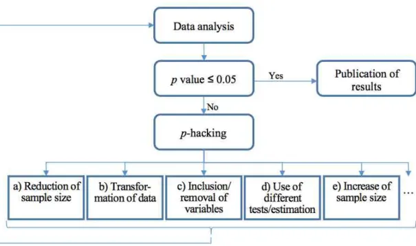
Figure 1 provides a brief overview of the manifold p-hacking possibilities, i.e., the versatile choices and interventions that a significance-pursuing researcher might be tempted to adopt even though they are not justified in regards to content18.
a. Exploratory reduction of sample size: Significance-pursuing researchers might be tempted to adopt one of the following interventions: first, they might explore in a trial-and-error process how p values can be reduced by removing data from the analysis on the seemingly justifiable grounds of being “outliers“. Second, in particular when disposing of large samples, researchers might be tempted to explore which p values they can obtain in a repeated analysis of data subsets. Imagine, for illustration, that a sample of 3,600 pigs is divided into 20 subgroups of 180
12 The term p-hacking is ascribed to Simmons et al. ([15] p.1359) who state: “[…] it is unacceptably easy to publish ‘statistically significant’ evidence
consistent with any hypothesis. The culprit is a construct we refer to as researcher degrees of freedom. In the course of collecting and analyzing data, researchers have many decisions to make: Should more data be collected? Should some observations be excluded? […] it is common (and accepted practice) for researchers to explore various analytic alternatives, to search for a combination that yields ‘statistical significance’, and to then report only what ‘worked’. The problem, of course, is that the likelihood of at least one (of many) analyses producing a falsely positive finding at the 5% level is necessarily greater than 5%".
13 Besides p-hacking (“significance pursuing behaviour”) and a poor understanding of p values, every research process is threatened with a variety of
other errors (measurement errors, inappropriate distributional assumptions, inadequate model selection, ill-founded equation of correlations with cause-effect relationships, etc.) that might lead to false conclusions. While they can cause serious problems in many analyses, the discussion of these latter types of errors is not this paper’s concern.
14 In the SPSS menu “Automatic linear modelling,” for example, users can chose the item “Automatically prepare data". This item includes several
pigs each. In every subgroup, a first partition of 90 pigs is fattened with the conventional feed CF; the other 90 pigs in each subgroup are also fattened with the conventional feed. The feed given to the second partition in each subgroup is marked, however, with one of 20 different food colourings that have no effect on fattening result. Nonetheless, the researcher is quite likely to find that, in at least one of the 20 subgroups, the coloured feed – for example, the one with the feed marked green – has a “statistically significant” effect. If the researcher then selectively reports this “result” under the heading “Pigs grow better with green feed,” then we have a serious case of self-serving p-hacking and a false discovery19.
b. Exploratory transformation of data: Even if sample size is not manipulated, data-related options of p-hacking remain. Researchers might be tempted, for example, to check whether certain data transformations produce lower p values than the
original data. Three common points of attack exist: the first one is to downgrade the measurements scales. An example would be to use ordered age classes rather than measuring an individual’s age in years. A second approach is to transform data to logarithms. A third one is to generate “new” variables from the original data. For example, if a researcher wants to analyse the influence of death penalty on murder there may be several modelling choices including not only the number of executions but also ratios such as executions per death sentence or executions per capita. Of course, any of these manipulations may be appropriate and justified by reasons related to the research question and the data structure. However, we are facing an overestimation of the validity of empirical evidence caused by p-hacking if these data manipulations are driven by significance-pursuing behaviour.
c. Exploratory inclusion/removal of variables: Even
15 As early as 30 years ago, Brandes pointed out that growing computing capacities and the increasing availability of sophisticated estimation procedures
generate a problematic room for manoeuvre in the design and choice of analytical alternatives: “The manifold possibilities of error compensation, on the one hand, and of model design, on the other, cause a dilemma that is difficult to resolve: The empirical econometrician who is a virtuoso of his methodological tool kit will frequently be able to confirm exactly those hypotheses that he is predetermined to confirm” (Brandes [28] p.78; non-authorised translation).
16 Simmons et al. ([15] p.1359-1360) comment on this as follows: “This exploratory behavior [i.e., p-hacking] is not the by-product of malicious intent, but
rather the result of two factors: (a) ambiguity in how best to make these decisions and (b) the researcher’s desire to find a statistically significant result. A large body of literature documents that people are self-serving in their interpretation of ambiguous information and remarkably adept at reaching justifiable conclusions that mesh with their desires […]. This literature suggests that when we as researchers face ambiguous analytic decisions, we will tend to conclude, with convincing self-justification, that the appropriate decisions are those that result in statistical significance (p ≤ .05)".
FIGURE 1. The manifold possibilities of p-hacking.
if original sample size and data are left unaltered, there is still scope for p-hacking because the choice of variables to be included into a regression model is also often ambiguous. This applies to control variables as well as to the manifest variables that are used to measure the latent constructs of the analysis. Significance pursuing researchers might be tempted to mine for and exclusively report the variable combination that yields low p values20. Imagine, for example, that a researcher wants to study how people’s attitudes towards organic farming affect their willingness to pay for organic products and that the information on attitude (= latent variable) is collected via several Likert-scaled survey items (= manifest variables). We are undoubtedly facing a distortion and an overestimation of the empirical evidence if the researcher mines for an item for “attitude” until he finds one that produces a “significant” result. The fact is not brought to light, however, if the researcher, for “marketing reasons,” reports only the convenient analysis that produced a “significant” result.
d. Exploratory use of tests/estimation models: Beyond the manipulation of data and variables, the ambiguities in the selection of appropriate statistical tests and fitting econometric models offer ample scope for self-serving decisions that yield “statistical significance”. Imagine, for example, that we are facing the ambiguous choice of whether to use a simple OLS estimation or rather a panel data model. We frequently have to make such decisions to the best of our knowledge, and it is often scientifically advisable to triangulate methods and openly compare the results of different approaches. However, the rules of good scientific practice are occasionally broken in this respect as well. That is, the data analysis is not performed as planned in a prior study design but ad hoc adjusted according to the criterion of which analytical model yields low p values. Transparency, which is the prerequisite of meaningful scientific communication, is completely lost when the results of competing models that have been used in the analysis are neither explicitly
reported nor comparatively discussed. In other words, just as other significance-pursuing behaviours, p-hacking regarding the selection of estimation models introduces biases that, in turn, lead to an inflation of the empirical evidence.
e. Exploratory increase of sample size: Last but not least, we have to deal with the “post-design” increase of sample size. Little awareness seems to exist that it is p-hacking if researchers ad hoc increase sample size when the original sample has yielded “disappointing” p values21. A general feeling that larger samples are better anyway may contribute to this lacking awareness. As other self-serving manipulations, the increase of sample size depending on “significance” introduces bias and inflates empirical evidence. The bias follows from the fact that the decision to collect more data is taken only if the original sample failed to produce low p values. If the follow-up data collection were carried out irrespective of whether significant results had been found or not, no bias would be produced because we would also have cases in which formerly significant results turn out not significant after the follow-up data collection. In other words, one would produce exactly the same (unbiased) results as in a study design with an a priori larger sample size.
To avoid misunderstandings one should note that exploration is not per se a problem. The question is whether we are dealing with an exploratory data analysis aimed at identifying correlations and generating hypotheses or a confirmatory data analysis aimed at testing hypotheses. An exploration of interesting correlations that might induce the generation of new hypotheses is an important primary step of the research process. We can thence understand “p-hacking” as a problem that arises when the two subsequent steps “exploratory data analysis” and “confirmatory data analysis” are conceptually confused and eventually even conducted with the same data. After an exploratory analysis, the resulting hypotheses have to be tested with a new set of data22. The term “hypothesis testing” must be avoided altogether in exploratory analysis since an exploratory study can only provide indications for the generation of hypotheses. Using the term “statistically
17 Nuzzo ([18] p.152), for example, writes in Nature: “Perhaps the worst fallacy is the kind of self-deception for which psychologist Uri Simonsohn of
the University of Pennsylvania and his colleagues have popularized the term P-hacking; it is also known as data-dredging, snooping, fishing, significance-chasing, and double-dipping. ‘P-hacking’, says Simonsohn, ‘is trying multiple things until you get the desired result’ – even unconsciously".
18 Motulsky ([2] p.200) summarizes the p-hacking problem as follows: “[…] analyses are often performed as shown in Fig. 1. Collect and analyze some
significant” can also be misleading in exploratory studies where we do not yet have hypotheses. If it is nonetheless used in exploratory research, we would have to interpret it in line with Fisher’s dictum according to which low p values signify “worthy a second look” (see, Nuzzo 18 p.151) in terms of conducting further studies.
Problem 4: Semantic equation of the “error probability”
with the “false discovery rate”
In addition to improper p-hacking activities in the research process, imaginary discoveries and the present replication crisis have been associated with the fundamental misunderstanding that the p value indicates the probability of the null hypothesis23. That is, besides the confusion about “significant” and “important,” we are facing another semantically induced misunderstanding – a misunderstanding that is invited by the convention to denote the p value as “error probability” (or “probability of type I error”). Despite this unfortunate labelling, the p value does not denote the probability of the null hypothesis (no effect) being true; it consequently does not indicate either the actually interesting false discovery rate, i.e., the (a posteriori) probability of making a type I error when rejecting the null24. As already mentioned, the p value is only the conditional probability to observe a certain effect (or even a larger effect) in a random sample contingent on the hypothetical assumption that the null hypothesis (no effect) was true. It is important to be very clear about the fact that it is not possible to draw a “backward” conclusion about the probability of the null hypothesis within the frequentist p value framework25. For this reason, the understanding that p values can be used for testing hypotheses is not quite correct either; we cannot test hypotheses with p values (in terms of assessing their probability) because p values indicate only how probable a random realisation or more extreme ones are – based on the assumption that a certain hypothesis is true26.
To demonstrate this fact, imagine that we randomly draw one coin from a box of coins. The probability to draw an unfair coin is 1% and the probability to draw a fair coin is 99%. We a priori know that all unfair coins
have been manipulated [P(Head) = 0.75; P(Tail) = 0.25] and that all fair coins have equal probabilities [P(Head) = P(Tail) = 0.5] when being tossed. We now generate experimental data and toss our coin five times. Let us assume that we obtain five times Head. We know that, if the coin were fair (= no manipulation effect), the probability of obtaining “five times Head” is 3.125% (= 0.55) in frequent repetitions of the experiment “tossing the coin five times". This conditional probability is exactly what is expressed by the p value. It is not the probability of the null hypothesis, however, to have a fair coin (= no effect); and it consequently contains no information either about the probability of making an error when rejecting the null. To obtain this probability of interest, we need the additional information of how probable it is to obtain “five times Head” in frequent repetitions of the experiment “tossing the coin five times” if the coin were unfair. This probability is 23.73% (= 0.755). We also need to consider the a priori probabilities (also called “priors”) of 1% and 99%, respectively, to have drawn an unfair or a fair coin from the box in the first place. According to “Bayes’ Theorem”, the probability of wrongly rejecting the null hypothesis to have a fair coin (i.e., the false discovery rate or probability to make a fool of oneself) is 92.88% [= 0.03125 ∙ 0.99/ (0.03125 ∙ 0.99 + 0.2373 ∙ 0.01)]. It is noteworthy that, despite the low p value of 3.125%, the null hypothesis should not be rejected. This is due to the fact that, besides the information from the experiment, we have valuable a priori information that it is highly probable to have drawn a fair coin. The additional piece of information provided by the experimental data would only make us update the probability of having a fair coin in our hands from the prior 99% to now 92.88%.
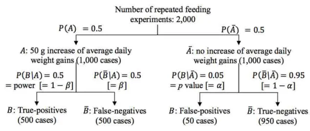
Figure 2 illustrates Bayes’ Theorem for our familiar pig-fattening example 2 where we have observed a difference in average daily weight gains of 50 g between the two feeding groups. We now assume that we have a group size of N = 88 pigs. In this case, the p value would be exactly 0.05. Following the notation in Figure 2, Ᾱ represents the null hypothesis “no increase in daily weight gains in the second group”, and A the alternative hypothesis “50 g increase in daily weight gains". The p value is the conditional probability P(B|Ᾱ) of observing
19 Kerr [29] terms this problem HARKing (Hypothesizing after the Result is Known) and Motulsky ([2] p.201) states in this context: “This is when you analyze
the data many different ways (say different subgroups), discover an intriguing relationship, and then publish the data so it appears that the hypothesis was stated before the data were collected […]. This is a form of multiple comparisons (Berry, 2007). Kriegeskorte and colleagues (2009) call this double dipping, as you are using the same data both to generate a hypothesis and to test it".
20 Many statistical software packages contain routines that facilitate a significance-oriented selection of variables (e.g., “Forward and backward effect
selection” in SAS). While such routines should not be used in confirmatory data analysis, their easy availability may misleadingly convey the impression to the inexperienced user that significance seeking trial-and-error procedures represent a sound standard. Using the easy routine might even seem so “normal” that users lose their ability to self-critically question their choice of variables.
21 Motulsky ([2] p.201) calls this form of p-hacking “Ad-Hoc Sample Size Selection” and explains: “This is when you did not choose a sample size in
the random realisation B “increased weight gain of 50 g or more” simply due to random sampling if there were no fattening enhancing effect. In our example, the computed p value (also called “false-positive rate”) equals , a symbol that is commonly used to denote an ex-ante defined maximum significance level (usually: 0.05). Our exemplary result of P(B|Ᾱ) = 0.05 = p = means that we have a 5% probability of finding a difference of 50 g or more due to random sampling error (i.e., by pure chance) when frequently repeating the feeding experiment with 88 pigs in each group if the null hypothesis Ᾱ “no increase in daily weight gains” were true.
If, in contrast, we assumed that the alternative hypothesis A were true, a random realisation B in the form of an increased weight gain of less than 50 g would be observed in 50% of cases when frequently repeating the feeding experiment with 88 pigs in each group. In these cases, we would find a p value of over 0.05 and thus wrongly not reject the null. That is, the conditional probability P(B|A) = , which is also called “false-negative rate,” amounts to 50%. Consequently, the true-positive rate P(B|A) =1 - , which is also called “power” and which
denotes the probability of finding a fattening enhancing effect of 50 g or more in repeated experiments if the effect exists, amounts to 50% as well.
To determine the actual probability of interest, i.e., the probability of making an error when rejecting the null, we need not only the false-positive rate P(B|Ᾱ) and the true-positive rate P(B|A) but also the a priori probabilities (“priors”) P(A) and P(Ᾱ) = 1 - P(A). The priors represent the probabilities that can be attributed to the hypotheses A and Ᾱ due to prior knowledge. In our example in Figure 2, we assume that no prior information is available that allows us to discriminate one hypothesis as being more probable than the other one. In following Laplace, we therefore assume both priors to be equal P(A) = P(Ᾱ) = 0.5.
If we now assume that we repeat the feeding experiment 2,000 times (with two fattening groups of 88 pigs, respectively), we have the following picture27: we can expect that a difference in group means of 50 g or more would be randomly realised in 50 repetitions (= P(Ᾱ) ∙ P(B|Ᾱ) ∙ 2,000 = 0.5 ∙ 0.05 ∙2,000) even if in fact there were no fattening enhancing effect. In other words, if the null were true, we would expect 50
false-22 In this context, Motulsky ([2] p.201) states very clearly: “Exploring your data can be a very useful way to generate hypotheses and make preliminary
conclusions, but all such analyses need to be clearly labeled [as preliminary or exploratory], and then retested with new data”. Gigerenzer and Marewski ([30] p.434-435) criticize the absence of differentiation between generating and evaluating hypotheses under the keyword “Surrogate Science” with “Hypotheses Finding is Presented as Hypotheses Testing".
23 It seems that this misinterpretation is also both pervasive and persistent. Even back in the 1980s, Sedlmeier and Gigerenzer ([7] p.314) cited a study that
had shown the widespread distribution of this misconception: “Oakes (1986) tested 70 academic psychologists and reported that 96% held the erroneous opinion that the level of significance specified the probability that either H0 or H1 was true". Cohen [31] coins this misconception “inverse probability error” and Nickerson ([13] p.251) writes: “The belief that p is the probability that the null hypothesis is true is unquestionably false. However, as Berger and Sellke (1987) have pointed out ‘like it or not, people do hypothesis testing to obtain evidence as to whether or not the hypotheses are true, and it is hard to fault the vast majority of nonspecialists […]. This is especially so since we know of no elementary textbooks that teach that p = 0.05 is at best very weak evidence against H0’ (p.114)”. In 2014, Motulsky ([2] p.204) still summarises the situation as follows: “The 5% significance threshold is often misunderstood. […] Many scientists mistakenly believe that the chance of making a false-positive conclusion is 5%. In fact, in many situations, the chance of making a type I false-positive conclusion is much higher than 5%".
FIGURE 2. True and false positives and negatives and the a posteriori probability of a type I error.
positives in which we would mistakenly reject the null and conclude that there is a difference. In contrast, if in fact the difference were 50 g, we would expect 500 true-positives because we would correctly reject the null hypothesis 500 times (= P(A) ∙ P(B|A) ∙ 2,000 = 0.5 ∙ 0.5 ∙ 2,000) and assume that there is an effect. In total, we would expect 550 positives in which the null hypothesis is rejected. Given the 50 false-positives among this total, we have a probability of P(Ᾱ|B) = 0.091 (= 50/550) to make a false discovery when rejecting the null. This corresponds to Bayes’ Theorem according to which the a posteriori probability P(Ᾱ|B) of making an error when rejecting the null (false discovery rate) is to be calculated as follows:
It is noteworthy that, despite a p value of 0.05, we have a false discovery rate (i.e., a probability of wrongly discarding the null) of more than 9%28.
To avoid comprehensible misunderstandings that might be invited by the unfortunate convention to use the words “p value” and “(type I) error probability” as interchangeable terms, two crucial facts need to be kept in mind:
1. Despite the confusing labelling, the so-called “error probability” does not give any information about the probability of committing an error when rejecting the null. In other words, the p value is not identical with the false discovery rate, i.e., the (a posteriori) probability of making a type I error when discarding the null hypothesis.
2. To determine the false discovery rate, one needs – besides the false positive rate (p value) – two types of additional information: the true-positive rate (1- ) of a concrete alternative hypothesis, and the priors P(A) and P(Ᾱ) which represent the information that was known before the study in question was carried out29,30.
A correct understanding of what p values tell us, and what not, is essential for adequately assessing the validity of statistical results. Despite the obvious limitations of the p value, the call for a general use of Bayesian approaches to determining the false discovery rate is in dispute. While Bayesian approaches force researchers to explicitly specify the presumed a priori knowledge, the very fact of using priors leaves much room for introducing subjective judgements into the process of research31. This has serious consequences because researchers can “easily” obtain a low false discovery rate P(Ᾱ|B) by using a high prior P(A), and vice versa. In our example in Figure 2, we would ceteris paribus obtain a false discovery rate P(Ᾱ|B) = 0.47 (= 90/(90+100)) if we assumed priors P(Ᾱ) = 0.9 = 1 - P(A). Against this background, the main criticism addressed at Bayesian approaches can be summarised as follows: while the request to keep the false discovery rate below a maximum level is justified, one can bring about any conclusion, independent of the chosen level, by choosing arbitrary priors that govern whether the null is rejected or not.
It is definitely true that choosing a smaller prior P(A) ceteris paribus increases the false discovery rate. However, such an “isolated” and arbitrary change of the prior P(A) is neither reasonable nor admissible. A prior is always to reflect at its best the a priori knowledge that is available with regard to the research hypothesis. Reducing the a priori probability P(A) will thus have to be accompanied by the choice of a less probable alternative hypothesis A. In our fattening experiment, the alternative hypothesis could read, for example, “70 g difference in daily weight gains". A less probable alternative hypothesis, in turn, increases the power 1- ; and an increased power reduces the false discovery rate. A consistent specification of both the hypothesis A and the associated prior P(A) thence tend to cancel each other out.
While Bayesian approaches have their problems due to subjective priors, conventional approaches to analysing data exhibit outright inconsistencies. The convention to reject the null hypothesis of “no effect” based on the condition that a pre-set significance threshold (e.g., p = 0.05) is met, is not consistent with the request to keep
24 To emphasise the poignancy of the problem, Colquhoun [1] calls the false discovery rate the “probability to make a fool of oneself” when rejecting the
null hypothesis.
25 Nuzzo ([18] p.151) stresses this fact by referring to a researcher who found a p value of 0.01: “Most scientists would look at his original P value of
0.01 and say that there was just a 1% chance of his result being a false alarm. But they would be wrong. The p value cannot say this: all it can do is summarize the data assuming a specific null hypothesis. It cannot work backwards and make statements about the underlying reality. That requires another piece of information: the odds that a real effect was there in the first place".
26 Kline ([12] p.14) unambiguously remarks: “[…] p values merely estimate the conditional probability of the data under a statistical hypothesis–the null
hypothesis–[…]. In fact, p values do not directly ‘test’ any hypothesis at all, but they are often misinterpreted as though they describe hypotheses instead of data".
27Contrary to the coin tossing example, the prior information here, as in many other cases, is not an objectively known probability of two possible events.
the false discovery rate below a unique level32. Depending on prior and power, identical (and possibly small) p values may imply very different (and possibly unacceptably high) false discovery rates (cf., our coin tossing example). Although the p value is not the same as the false discovery rate, we can make the qualitative statement that the false discovery rate decreases ceteris paribus with a decreasing p value. We also know that the larger the sample size and the less a priori knowledge we have, the better the p value approximates the false discovery rate33.
It is interesting that external researchers (i.e., researchers who are not involved in a given study) rarely equate the p value with the false discovery rate when other researchers find a “statistically significant” effect that contradicts the up-to-date knowledge. It is as if external researchers included the essentials of Bayes’ Theorem into a qualitative line of reasoning in such cases. Accordingly, they treat even very low p values with healthy scepticism and are not willing to discard their prior knowledge due to a single study – even if its analytical approach stands critical examination. In other words, they do not mistake the so called “error probability” for the probability of the null hypothesis and therefore the false discovery rate. Instead, leaving the frequentist p value framework, they use the Bayesian rationale and only ask to what extent they must “update” their former knowledge in light of the findings from the new study. Slightly more formal, the argument runs as follows: if well-founded scientific knowledge indicates a prior P(Ᾱ) of almost 100%, then the a posteriori probability of the null hypothesis remains nearly 100% [(P(Ᾱ|B) ≈ 1] even if a low p value is found in a study. We would consequently have a false discovery rate of nearly 100% when rejecting the null, even though the effect was found to be “highly statistically significant". It is thus also formally correct not to reject the null hypothesis solely on the basis of a low p value.
Suggested solutions and outlook
In the recent past, criticisms of misinterpretations and manipulations of the p value have increasingly been voiced in the scientific community34, and there appears to be little contention that the status quo of scientific reporting
is much less than perfect. Aiming to reduce the rate of false discoveries in the future, a plethora of suggestions have been made of how academic teachers and authors of textbooks, (junior) researchers and authors of scientific papers as well as journal reviewers and editors can contribute to the mitigation of the problem. In the following, we systematically describe the most relevant of these propositions in relation to the above-described problems.
While mixing up “significant” and “large/strong” appears to be an obstinate problem especially in oral arguments (and even among experienced researchers), it is an easy-to-understand problem in principle. It is hence also easy to avoid and prevent, provided that the problem awareness regarding this “semantically seducing” misinterpretation can be increased. However, some of the suggestions made in the literature might have limited prospects of being accepted in the scientific community. Armstrong [35], Motulsky [2], and Colquhoun [1], for example, propose banning the word “significant” in scientific publications altogether. Given the long tradition and omnipresence of the term, it seems doubtful whether this proposal has a chance of being accepted in the scientific community. Explicitly addressing the semantically induced misunderstanding of the term “significant” in academic teaching might have a more realistic prospect of success. Students and junior researchers need to be systematically warned and requested not to colloquially equate “significant” with “large/strong” and to use the complete wording “statistically significant” whenever the omission of the adjective “statistically” causes the risk of confusion (cf., Mittag and Thompson [36]). On the level of scientific journals, reviewers should explicitly be required to pay attention to lacking semantic clarity and colloquial confusion connected to the word “significant". Journals could also use their guidelines to request authors to discuss the effect size whenever meaningful units of measurement are used. This would already be a definite step in the right direction, a step that could be made with little effort (Goodmann [14]). In addition, as recommended by the American Psychological Association [37], journal guidelines could require authors to report confidence intervals, thus forcing them to communicate information regarding the effect size in an easily comprehensible way without loss of information on significance. Using the label
28 In hypothesis testing, predefined thresholds of 0.05 (for the significance level) and of 0.8 (for the power) are suggested in the literature (see, e.g., Sedlmeier
“statistical cognition”, Cumming ([11] p.11-13) points out that presenting information in a more intelligible form such as confidence intervals reduces misconceptions that are frequently caused even among researchers themselves when the less intelligible p values are reported.
False interpretations of p values above the significance level can also be easily counteracted in teaching. For this purpose, students and junior researchers must be acquainted with logical reasoning and the law of the excluded middle. Since it is easy to comprehend the problem from a logical point of view, it should be possible to successfully teach young scientists to avoid false dichotomies. One step further, on the journal level, reviewers should be explicitly asked to reject formulations that insinuate the false interpretation “if p > 0.05, then the null hypothesis is confirmed". Because this logical fallacy can easily be detected, it should be possible to ensure a stringent standard in the reviewing process. When it comes to the perception of research findings by the interested public, false dichotomies might be an obstinate problem that is more difficult to remediate. It is often very difficult to impart to diverse “users” of scientific findings such as specialised journalists or politicians that the scientific label “not significant” must by no means be interpreted as an indication of little or no effect. The problem can partly be attributed to the phenomenon that many actors who are involved in the struggle for public attention and recognition prefer an attention-grabbing, albeit wrong message “X has no effect on Y!” to a “bland” statement that we simply have found no conclusive evidence yet and need further research. Especially if research findings play an important role in public debates and political decisions, researchers face not only the great challenge but also the moral obligation to correct such misinterpretations, and repeatedly so if necessary.
The p-hacking problem is more difficult to solve than the first two problems. This is because it does not represent semantic mix-ups or logical fallacies that can be easily identified, but a careless disregard of good scientific practice or even outright scientific misconduct in the very process of research. It is hence difficult to detect from the outside. Besides raising the awareness of students and junior researchers, the proposals put forth by various parties for mitigating the p-hacking problem hence
mainly target the publishing practices of scientific journals. A first recommendation is to require authors to clearly state in each paper’s introductory section whether their study is exploratory in nature (i.e., aimed at generating hypotheses) or whether it is confirmatory (i.e., aimed at testing hypotheses). The two steps “exploratory analysis” and “confirmatory analysis” must not be mixed up. They are conceptually distinct, sequential in nature, and have to be carried out with different data (see e.g., Marino [38] or Motulsky[2])35. An even further-going proposal is to make researchers carry out at least one internal replication study with new data as a default before publishing. A second recommendation is to require authors to make all raw data and a detailed documentation of all analytical steps (including data transformations, etc.) publicly available (see e.g., Simmons et al. [15]). A still further-reaching proposal is to require researchers to register all studies and deposit both the complete data and the concrete study design on a public repository before starting the analysis. Obviously, such proposals raise the question of who is able and willing to take the time to examine all this material. The third recommendation is to oblige authors to underwrite – as with “no competing interests” statements – a formal “no p-hacking” declaration as a default (see e.g., Simmons et al. [39]). Such a formal self-commitment is believed to strengthen the normative power (“norm appeal”) of good scientific practice rules. The problem with such a declaration is seen in the difficulty to unambiguously define the practices that qualify as p-hacking without considering the specific context of each study. It is hence unclear which practices exactly should be outlawed on the grounds of clearly inflating the strength of empirical evidence. Furthermore, given the perverse but system-induced “publish or perish” conditions that most researchers face today, it is questionable whether this attempt to strengthen the norm appeal is sufficient to solve the problem. However, given the less than perfect status quo, we agree with Simmons et al. ([39] p.6) that “changes need not to be assessed in terms of their perfection, but merely in terms of their improvement“. A fourth recommendation takes up the general discussion about publication biases. Focusing on medical research, but certainly also true in other disciplines, Colquhoun ([1] p.11) comments on the situation as follows: “The reluctance
29 Motulsky ([2] p.204) gets to the heart of the issue: “Statistical hypothesis testing [based on conventional practice] ‘does not tell us what we want to know,
and we so much want to know what we want to know that, out of desperation, we nevertheless believe that it does’ (Cohen, 1994). […] The question we want to answer is: Given these data, how likely is the null hypothesis? The question that a p value answers is: Assuming the null hypothesis is true, how unlikely are these data? These two questions are distinct, and so have distinct answers".
30 Instead of focusing on the false discovery rate, researchers occasionally report the ratio of the two a-posteriori probabilities P(A|B)/P(Ᾱ|B). This ratio,
of many journals (and many authors) to publish negative results biases the whole literature in favour of positive results“. Against this background, parts of the scientific community call for a general change in attitude towards “negative” results and replication studies and demand that they should be given more scientific recognition and a higher chance of publication by editors and reviewers36,37.
Mixing up the so called “error probability” (p value) and the “false discovery rate” is persevering and difficult to counteract because common language usage strongly invites this misunderstanding. What is more, the fact that both the p value and the false discovery rate are conditional probabilities may erect additional barriers to understanding. According to Gigerenzer [44], many people have troubles in grasping the very concept of probability and, in particular, the meaning of conditional probabilities. This is why they are so vulnerable to what Cohen [31] has called the “inverse probability error“. Again, better teaching is the prerequisite for improvement. Better teaching needs to be based on illustrative and intuitive examples that sharpen up awareness and ensure that students and young researchers acquire a deeply entrenched understanding of the distinct meanings of these two distinct conditional probabilities. However, even if such an understanding flourishes, the question remains of how researchers should “do” inferential statistics and evaluate their empirical evidence in the future. One argument for simply going on with displaying the p value is the “comfortable” nature of the seemingly clear guidance for assessing inferential validity that it offers to researchers and reviewers alike. However, an exclusive reliance on the p value that, as we know, solely results from the mean, variability, and size of a random sample, would not only mean to disregard the effect size in the evaluation, but also to discard the whole body of prior knowledge that exists with respect to the question under investigation. The advancement of science is inevitably based on (a usually large body of) preliminary work and prior knowledge that needs to be systematically contrasted and brought together with the incremental findings of new research – a fact that finds its succinct expression in the metaphor of the “dwarves standing on the shoulders of giants". Accordingly, most researchers will evaluate results that reproduce well-established earlier findings – even if they are not quite
statistically significant – as a small additional step towards confirming earlier findings. In contrast, they will consider statistically significant findings of a new study that come as a complete surprise with great suspicion even if they have no grounds to suspect biases in the data and the analytical design. This scepticism corresponds to the implicit thinking that a random sampling error of 5% is not so negligible after all, and that the null hypothesis therefore is probably true despite the surprising results of the new study. This scepticism can also be considered as a reasoning that goes beyond the frequentist p value framework and uses a qualitative argument along Bayes’ Theorem without formally computing the false discovery rate. This in mind, the following criticism of Leamer ([45] p.37) from over 30 years ago may have to be seen in a new and favourable light: “Hardly anyone takes data analyses seriously. Or perhaps more accurately, hardly anyone takes anyone else’s data analyses seriously“38. Formalising this criticism would force scientists to specify their priors, which, in turn, would facilitate the computation of the false discovery rate instead of having to rely on qualitative reasoning. With a view of the commonly hesitant attitude towards change, suggestions have been made to introduce a stepwise approach that combines a quick p value based validation with a more comprehensive approach based on Bayes’ Theorem whenever useful or necessary (see Nickerson [13] p.290-291). This could be coined as the attempt to “do the new thing without neglecting the old one". Retaining the conventional procedure would certainly suit those researchers who feel uneasy about the inevitably subjective determination of priors. An incremental formal reasoning along Bayes’ Theorem would have the advantage to disclose implicit priors, thus laying open prior judgement based on prejudices and decrepit paradigms as well as an imprudent lack of scientific scepticism. In other words, we would see an increase of transparency in the intersubjective communication between scientists. This holds especially if systematic variant calculations with regard to priors are provided (see Zyphur and Oswald [34]) that clearly show what scientists should dispute over when it comes to inferential conclusions. In this context, Ioannidis ([10] p.0701) states: “Even though these assumptions would be considerably subjective, they would still be very useful in interpreting research claims
31 Regarding this issue, Simmons et al. ([15] p.7) argue: “Although the Bayesian approach has many virtues, it actually increases researcher degrees of
freedom. First, it offers a new set of analyses […] that authors could flexibly try out on their data. Second, Bayesian statistics require making additional judgments (e.g., the prior distribution) on a case-by-case basis, providing yet more researcher degrees of freedom".
32 As one of few economic papers, a recent contribution in the field of experimental economics (Maniadis et al. [33] p.278) comments on this as follows:
“The common reliance on statistical significance as the sole criterion leads to an excessive number of false positives. […] the decision about whether to call a finding noteworthy, or deserving of great attention, should be based on the estimated probability that the finding represents a true association [i.e., the positive predictive value =1- false discovery rate], which follows directly from the observed p value, the power of the design, the prior probability of the hypothesis, and the tolerance for false positives".
33 Zyphur and Oswald [34] describe that, as sample sizes increases, the p value will approximate the false discovery rate according to Bayesian analysis