Generalized Cyclic Open Shop Scheduling and a Hybrid Algorithm

Vol. 1, No. 4, pp 345-359 Winter 2008

Generalized Cyclic Open Shop Scheduling and a Hybrid Algorithm

Mohammad Modarres1*, Mahsa Ghandehari

Industrial Engineering Department, Sharif University of Technology, Tehran, Iran ABSTRACT

In this paper, we first introduce a generalized version of open shop scheduling (OSS), called generalized cyclic open shop scheduling (GCOSS) and then develop a hybrid method of metaheuristic to solve this problem. Open shop scheduling is concerned with processing n

jobs on m machines, where each job has exactly m operations and operation

i

of each job has to be processed on machine

i

. However, in our proposed model of GCOSS, processing each operation needs more than one machine (or other resources) simultaneously. Furthermore, the schedule is repeated more than once. It is known that OSS is NP-hard. Therefore, for obtaining a good solution for GCOSS, which is obviously NP-hard, a hybrid algorithm is also developed. This method is constructed by hybridizing ant colony optimization (ACO), beam search and linear programming (LP). To verify the accuracy of the method, we also compare the results of this algorithm with the optimal solution for some special problems.

Key words: Open shop scheduling; Cyclic open shop scheduling; Metaheuristic; ACO, Beam search.

1. INTRODUCTION

Open shop scheduling problem has a wide range of applications in many industries (Liaw, 2003). However, the assumption that each job has exactly m operations and its ith operation has to be processed on machine

i

does not hold for many real-world problems. Therefore, in order to make it more realistic, we introduce a new version of OSS by relaxing these restrictive assumptions. In this version of generalized cyclic open shop scheduling (GCOSS), it is assumed each operation needs more than one machine or resources (such as technician or special tools) simultaneously. OSS problems (and consequently GCOSS) are shown to be NP-Hard (Garey and Johnson, 1979). As a matter of fact, the structure of OSS is larger than any other typical scheduling problem. Thus, in this paper we develop an algorithm based on hybridizing ACO, linear programming and Beam search.

To our knowledge, a similar approach to model cyclic open shop scheduling problems, even for a single period problem, has not been applied previously in the literature, although the circular coloring concept has been applied in other scheduling problems. The only paper in the literature, regarding cyclic open shop scheduling is by Kubale and Nadolski (2005). They showed this problem is NP-hard for a 3-processor system but it is polynomially solvable for a 2-processor one.

*

They proved if a given open shop can be scheduled in 3 time units then it is polynomially solvable. They also proved that in a compact open shop, the problem of minimizing

C

_max for 2-processor to determine the existence of a legal schedule is also NP-hard.

Our paper is organized as follows. Section 2 presents the definition and the structure of the problem. In section 3, we describe how to apply the concept of graph circular coloring to formulate this problem. In section 4, a metaheuristic algorithm is developed to tackle this problem. We provide an experimental evaluation in section 5.

2. GENERALIZED CYCLIC OPEN SHOP SCHEDULING PROBLEM

The generalized cyclic open shop scheduling (GCOSS) problem is defined as follows. Consider a manufacturing system in which a number of jobs must be processed. Each job consists of several operations. Each operation must be processed without preemption, i.e. the processing of an operation cannot be interrupted. Like OSS, operations in each job can be processed in any order. Each operation needs to be processed on a number of machines (or needs a set of resources) simultaneously. The processing time of each operation is a given specified time. Each machine can process at most one operation at a time. Similarly, each resource cannot be used by more than one operation at a time. Operations belonging to the same job cannot be processed simultaneously. We use the following notation to formulate this problem.

}

,...,

,

{

M

1

M

2

M

m

M

=

the set of different machines (or dedicated resources);

}

,...,

,

{

J

1

J

2

J

n

J

=

the set of different jobs to be processed; j

n

the number of different operations of job

j

;

}

,...,

,

{

j1 j2 jn_j

j

o

o

o

O

=

the set of operations of job

j

; ji

m

the set of machines (or resources) that operation o_ji needs for processing simultaneously;

O the set of all operations ;

j j J

O

O

∈

=

∑

_{the total number of operations.}

Each permutation of operations represents a solution to this problem. The search space can easily be defined as the set of all permutations of all operations. Function

P

:

O

→

IR

+ assigns the processing time to operations.

There are several criteria to measure the cost of a solution. In this paper, we deal with makespan minimization while the process can be repeated more than once. In fact, we search for a solution where the makespan is minimized in a cyclic version of the problem. Adopting the other objective functions does not change the structure of the model.

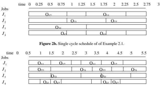
Example 2.1: in this example we represent an instance of the GCOSS with four jobs

of

J

=

{

J

1

,

J

2

,

J

3

,

J

4

}

and the operations of

O

=

{

o

11

,

o

12

,

o

21

,

o

22

,

o

31

,

o

41

,

o

42

}

. There are three different machines

M

1

,

M

2

,

M

3,and three operators

M

4

M

5

,

M

6. Thus, the set of resources is

}

,

,

,

,

,

{

M

1

M

2

M

3

M

4

M

5

M

6

Job J₁ consists of operationso₁₁ando₁₂, or by our notation, O₁ ={o₁₁,o₁₂}. Similarly,

} ,

{ 21 22

2 o o

O = ,

O

3

=

{

o

31

}

andO4 ={o41,o42}. Operation o11 must be processed on machine 1

M under supervising operatorM4, or by our notation, m11 ={M1,M4}. Similarly,

}

,

{

},

,

{

},

,

{

},

,

{

},

,

{

},

,

{

6 1 42 5 2 41 4 3 31 6 3 22 5 2 21 5 2 12

M

M

m

M

M

m

M

M

m

M

M

m

M

M

m

M

M

m

=

=

=

=

=

=

Table 2.1. Processing times of operations,

p

_ij

3. GRAPHICAL MODEL OF THE PROBLEM

An open shop scheduling (as well as a generalized cyclic open shop scheduling problem) can be represented by a graph.

Definition 3.1: A pair of operations is called related (or incompatible) if either both belong to the

same job or if they need at least a common machine (or resource) to be processed. Let

R

_ji

represent the set of all operations related to o_ji.

Graphical model of OSS. An OSS problem can be modeled as a bipartite graph. In this graph,

each edge represents an operation with a weight of

p

jiwhich is equal to the processing time of operation

j

on machine

i

.

Graphical model of GCOSS. Since in GCOSS more than one machine is needed to process an

operation, this problem cannot be modeled as a bipartite graph anymore. Thus, this problem is modeled as a weighted graph

G

=

(

V

,

E

)

, where V and

E

represent the set of nodes and edges, respectively. In this graph, an operation, say

o

_ji, is represented as a node of this graph, while the weight of this node is equal to the processing time of this operation and obviouslyV = O . By definition 1, there exists an edge between a pair of nodes, if and only if the corresponding operations are related.

It can be shown easily that the chromatic number of this weighted graph is equal to the minimal makespan of the schedule.

If the production is repeated, in some cases the makespan can be improved by making the schedule compact. This is called cyclic schedule. In this case, it can be shown that the minimal makespan of the schedule is equal to the circular chromatic number of weighted graphG. The circular chromatic number of weighted graph is defined as follows.

j

i

1 2

1 1 1

2 1 1

3 1.5 --

Definition 3.2. Consider a weighted graph of

(

G

,

w

)

with vertex set V and edge set

E

, where :

w V →+are weights of vertices. Then, the r-circular coloring of this graph is a mapping

Γ

of V to open arc of an Euclidean circle C of length r, such that:

i)

Γ

(

x

)

and

Γ

(

y

)

are disjoint if

(

x

,

y

)

∈

E

(

G

)

.

ii) the length of

Γ

(

x

)

is at least

w

(

x

)

for all vertices x∈V.

The circular-chromatic number

χ

c

(

G

,

w

)

of weighted graph

(

G

,

w

)

is

χ

c

(

G

,

w

)

= Inf{r : there is an r circular coloring of

(

G

,

w

)

}.

If the weight function takes constant value 1, then

χ

c

(

G

)

=

χ

c

(

G

,

w

)

, (Zhu, 1992) . It is proved

that

χ

_c

(

G

,

w

)

is always attainable (Deuber and Zhu, 1997).

We use the concept of graph circular coloring to formulate GCOSS. The following mathematical model represents this problem, where

t

_ji

,

∀

i j

,

are decision variables indicating the starting time of operation

o

ji and

r

is the makespan.

In subsequent section, a linear model which is the relaxed version of this formulation is applied to construct our proposed algorithm of Beam-ACO.

,

.

.

.

ji

ji j i ji jj ii ji j i

ji j i j i jj ii ji j i

ji j i jij i ji

Min

Z

r

r

t

i j

t

t

p

M y

o

R

t

t

r

p

M y

o

R

t

t

M y

o

′ ′ ′ ′ ′ ′

′ ′ ′ ′ ′ ′ ′ ′

′ ′ ′ ′

=

≥

∀

−

≥

−

∀

∈

−

≥ −

+

∀

∈

≥

−

∀

∈

1

{0,1}

, ,

,

j i

jij i j i ji ji j i

jij i

R

y

y

o

R

y

j i j i

′ ′

′ ′ ′ ′ ′ ′

′ ′

+

=

∀

∈

′ ′

∈

∀

Where M represents a large number.

The graph of Figure 2a corresponds to the GCOSS problem of Example 2.1. Figure 2b and Figure 2c represent a single cycle and periodic schedule of this problem, respectively.

Figure 2a. Graphical representation of Example 2.1.

O11

O12

O21 O22

O31

O41 O42

time 0 0.25 0.5 0.75 1 1.25 1.5 1.75 2 2.25 2.5 2.75 3 Jobs

1 J

2 J

3

J

4 J

Figure 2b. Single cycle schedule of of Example 2.1.

time 0 0.5 1 1.5 2 2.5 3 3.5 4 4.5 5 5.5 Jobs

1 J

2 J

3

J

4 J

Figure 2c. Periodic schedule of of Example 2.1.

4. HYBRID ALGORITHM

In this section, we introduce an algorithm developed for obtaining a good (near optimal) solution of GCOSS problems. This algorithm is constructed by hybridizing ant colony optimization (ACO), Beam search and a local search technique. Both ACO and beam search belong to the category of constructive methods which obtain a complete solution by generating a sequence of partial solutions. A partial solution is defined as a subset of a solution in which only some variables are fixed, but not all. After assigning the value for all variables, the solution is called a complete one. In fact, rather than moving from a solution to another one, in ACO (and also in search beam), the number of assigned variables is increased in subsequent iterations (Blum, 2005). At each step, partial solutions are extended by adding a component from an allowable set. This procedure is ended when either a partial solution can not be extended any more or become a complete feasible solution.

Before presenting the proposed algorithm, we review ant colony optimization (ACO) and beam search briefly.

4.1. Ant colony optimization (ACO)

Ant colony optimization (ACO) is a metaheuristic to tackle hard combinatorial optimization problems. It was first proposed in the early 1990s (Dorigo and Stutzle, 2004. This algorithm is constructed on the basis of foraging behavior of real ants. In this algorithm, the solutions are constructed based on a probabilistic model, called pheromone model. Pheromone model consists of a set of parameters

τ

, called pheromone trail. The value of pheromone parameter is usually associated with the set of partial solutions obtained up to now.

At each step, a number of ants, say

n

_a, construct

n

_a partial solutions probabilistically. Some of the constructed solutions are used to update the pheromone values. These values along with another

O

31

O

21

O

22

O

12

O

11

O

42

O

41

O

31

O

31

O

22

O

21

O

22

O

21

O

11

O

12

O

11

O

12

parameter, called heuristic information, are used to determine the transition probabilities

)

(

),

,

|

(

c

c

N

s

p

P

τ

η

∀

∈

, where

s

_tp is the current partial solutions at step

t

and

N s

(

_tp

)

is the set of neighborhood of

s

_tp, (as will be defined later). Transition probabilities are used to select the next component of partial solution at each step of solution construction. A quantity named convergence factor is also computed whenever the pheromones are updated. This factor takes value 1 if the ants determine a common trail.

Actually the pheromone model leads ants to generate high quality solutions over time. Heuristic information is a weighting function

η

:

N

(

s

tp

)

→

IR

+and assigns a weight to each possible

extension of current partial solution

s

_tp. These weights reflect the benefit of extending a partial solution. The algorithm terminates, if the stopping conditions such as a maximum CPU time hold. For more information, the reader is referred to Dorigo and Stutzle, 2004.

4. 2. Beam search

Beam search (BS) is a classical tree search that was introduced in the context of scheduling and since then has been applied to many other combinatorial optimization problems successfully. This technique is an incomplete derivative of branch and bound algorithm (Ow and Morton, 1998). The central idea behind BS is to extend the partial solution in several possible ways. At each step, a partial solution from beam set

B

is extended at most in

k

ext possible ways. Each newly obtained partial solution is either a complete solution and is stored in the set of complete solution

B

C, or again a partial solution and is stored in the set of further extensible partial solution

B

ext. At the end of each step, when all members of

B

are extended, up to

k

bw(called beam width) solutions are selected from the set of

B

ext, based on the value of their lower bounds, provided

B

extis not empty. Actually, for each partial solution, a lower bound is computed for the objective function of all complete solutions which are constructed from this partial solution.

At the first step, the set beam

B

consists of only one partial solution, say

s

p

=<

o

₁₁

>

. The reason is that in a cyclic scheduling, the order of operations is not important. Thus, one operation is selected arbitrarily to build a schedule. This algorithm terminates when set

B

ext is empty.

One major difference between ACO and beam search is that in ACO the set of partial solutions is constructed probabilistically, while beam search is a method that solutions are constructed deterministically. We use a hybridized method to take advantage of the benefit of combining both ways of exploring the search space.

4. 3. The algorithm

Ant colony optimization is the basic framework of the proposed algorithm. In standard ACO a group of ants generate the partial solutions probabilistically by considering two guides, the pheromone values and the heuristic information. However, in this method by adopting beam search rules, a component is selected deterministically to append the solution. In fact, the probabilistic choice of another component to append a partial solution in ACO is replaced by the deterministic choice of beam search.

The best complete solutions are stored in two sets,

s

_bsand

S

_best representing the best solutions so far and the best solutions after the previous restart, respectively.

The main algorithm is called Beam-ACO (or simply Algorithm 1). However, another supporting algorithm, called Beam-ACO-Construction (or simply Algorithm 2), constructs the structure of the partial solution. Actually, it represents the steps of this probabilistic beam search.

Some components of Algorithm 1 are outlined in more details as follows.

Initialize pheromone values (

τ

): all pheromone values are initialized to 0.5, at the start of algorithm.

Beam-ACO-GCOSS solution construction (

τ

). From our notation, the set of all operations is represented by O. Let the current partial solution be

s

tp. Then, O is partitioned into two sets of

− t

O

and

O

_t+, where { | p}

t ji ji t

O− = o o ∈s and

O

_t+

=

O

|

O

_t−. Actually,

O

_t− represents the set of operations which are already fixed in the sequence of this partial solution and

O

t

+

is the set of operations which are still free and can be appended

If O_t+∩R_ji = ∅for an operationoji Ot

+

∈ , then oji is not related to any other remaining

operations. In that case, the position of this operation in the sequence is not important. Actually, this partial solution can be appended with the remaining operations in any arbitrary sequence. Therefore, we define the set of allowed operations (neighborhood of

s

_tp) as follows:

( _tp) { _ji | _{ji t} , _{ji t} }

N s ← o o ∈O+ R ∩O+ ≠ ∅

As mentioned before, the next operation in ACO is selected probabilistically. This is done by computing transition probabilities. Thus, it has to determine pheromone values and the weighting function that is called heuristic information. The pheromone values are computed by Algorithm 2. However, the weighting function (heuristic information) is defined as:

( )

1

(

,

) 1

(

)

(

)

1

(

,

) 1

p lk t

p

es ji t p

ji ji t

p o N s es lk t

t

o

s

o

o

N s

t

o

s

η

∈

+

←

∀

∈

+

∑

Where ( , p)

es ji t

t o s is the earliest starting time of ojiwith respect to the partial solution

p t

s

. At the beginning,

s

_tp has no operation. Then, the earliest starting of

N s

(

_tp

)

is 0.

The transition the probability of selecting o_ji∈N s( p)is defined as follows.

( )

(min

)

(

)

(

| , )

(

)

(min

)

(

)

j i ji t

j i lk t P

lk t

jij i ji

o R O _p

ji ji

lkj i lk o R O

o N s

o

p o

o

N s

o

α α

τ

η

τ η

τ

η

+ ′ ′ + ′ ′ ′ ′ ∈ ∩ ′ ′ ∈ ∩ ∈

←

∀

∈

∑

Clearly, if the minimum of τjij i′ ′ is lower than that of

o

lk , then

p o

(

ji

| , )

τ η

≤

p o

(

lk

τ η

, ).

It means that there is at least one operation left that probably should be scheduled before c=oji.

Let

α

be the adjusting factor which indicates the importance of pheromone values with respect to the heuristic information. Ø

4. 4. Algorithm 1, Beam-ACO for GCOSS problem

Input: an GCOSS problem instance

s

_bs

← < >

,

S

_best

← ∅

,

cf

←

0

Initialize pheromone values

(

τ

)

while termination condition not satisfied do

S

iter

←

Ø

for

j

=

1

to

n

a

S

iter

←

S

iter

∪

Beam-ACO solution construction

(

τ

)

end for

Apply local search

(

S

iter

)

(optional step)

Find the set of obtained best solutions

(

S

iter

)

Apply pheromone update

(

τ

,

S

best

,

s

bs

)

cf

←

compute convergence factor () if

cf

>

cf

_

lim

it

then

Reset pheromone values

(

τ

)

S

_best

← ∅

end if end while

output:

s

bs, a set of best solutions

S

bestfound

4. 5. Algorithm 2. Beam-ACO-Construct for structure of GCOSS solution.

Some details of Algorithm 2 are presented as follows.

Since our scheduling is a cyclic one, the first operation can be selected arbitrarily. So

s

₁p

=<

o

₁

>

.

Reduce to related( ( p), )

t ji

N s o : this procedure is used to restrict the neighborhood set, after the first extension of partial solution

s

tpwas performed. This is done as follows:

( _tp) { _{j i} ( _tp) | _{j i ji}} N s = o′ ′∈N s o ′ ′∈R

This effective procedure prevents the construction of permutations that have no effect on the final solution.

Rank the partial solution

s

_tp using a lower bound LB(.): we compute a lower bound from the definition of t_es(o_ji,s_tp).

As we said ( , p)

es ji t

t o s is the earliest starting time of operation oji with respect to the partial

solution

s

_tp. Thus, the earliest completion time ( , p)

es ji t

t o s of operation o_ji is ( , p)

es ji t ji

t o s +p . The approximate earliest completing time is constructed by extending

s

tp as follows:

}

,

max{

(.)

X

Y

LB

=

max p{ ( , ) ( )}

ji t tji p ji t o s o R

X tec o s p o

+

∈

∈

= +

∑

, max { ( )}

ji t tji o O

o R

Y − p o

+

∈ ∈

=

∑

Similar to the partition of O into

O

_t− and

O

_t+ , R_jiis also partitioned into two subsets of Rtji

+ _and

tji

R−.

Input data for

k

_bw and

k

_ext: }

10 | | , 1 max{ O

k_bw = and

k

_ext

=

{1,

N s

(

_tp

) / 2}.

The set of best solutions

(

S

iter

)

: The objective value of each solution in

S

itermust be determined and then a number of the best solutions equal to

max{

|

|

,1}

10

iter

S

are selected. However, To determine the objective value (makespan) of a solution <o1,o2,...,oO > where

O

o

k

∈

,

t

k

≥

t

k′

if

k

≥

k o

′

,

k

∈

R

k′

,

we use the following linear programming:

k k k k k k k k k k k

R

o

k

k

p

r

t

t

R

o

k

k

p

t

t

k

t

r

r

Z

Min

′ ′ ′ ′

∈

′

∀

−

≥

−

∈

′

∀

≥

−

∀

≥

=

;

,

;

,

Updating pheromone

τ

:

( ( , , ) )

( ,

ji j i jij i s S

jij i jij i

o o s

S

τ

τ

δ τ

τ τ ρ

′ ′ ′ ′

∈

′ ′ ′ ′

−

← +

∑

where δ(oji,oj i′ ′, )s =1 if oji is

scheduled before oj i' ' and δ(o oji, j i′ ′, )s =o, otherwise.

ρ

∈

[

0

,

1

]

is a constant called evaporation

rate.

Compute convergence factor:This numerical factor controls the algorithm. This factor is denoted as

cf

∈

[

0

,

1

]

and is computed as follows:

max min

max min

{ , }

2( 0.5)

( )

ji j i i

jij i ijij i o O o R

cf

τ τ τ τ τ τ τ

′ ′ ′ ′ ′ ′ ∈ ∈ − − ← − −

∑ ∑

Upper bound

τ

_maxand lower bound

τ

_min: to prevent the algorithm from converging to a local solution, as proposed by Stutzle and Hoos (2000), we set 0.01 and 0.09 as the lower and the upper bound of

τ

. After applying pheromone update rule, we check to make sure the pheromone remains within the range of

[

τ

_min

,

τ

_max

]

. When the pheromone values take their limited bound, then

cf

=

1

. The steps of Algorithm 2 are as follows.

Input: partial solution

s

1

=<

o

1

>

p

, beam width

k

bw, maximum number of extensions

k

ext

B

←

{

s

₁p

},

B

_C

←

,

t

←

1

while

B

≠

do

B

_ext

← ∅

for

s

tp

∈

B

do

count←1

N

(

s

_tp

)

←

PreSelect

(

N

(

s

_tp

))

while

count

≤

k

extAND

(

)

≠

p t

s

N

do

choose ( p)

ji t

o ∈N s with transition probability p o( _ji | , )τ η

s

tp₊1

←

extend

p t

s

by appending operationoji

( p) ( p) | { }

t t ji

N s ←N s o if N s( _tp)≠ ∅ then

{

1

}

p t ext ext

B

s

B

←

∪

₊ else

B

_c

←

B

_c

∪

{

s

_tp₊₁

}

end if

if count=1 then

N

(

s

_tp

)

←

Reduce To Related(N s( _tp),o_ji) end if

count←count+1

end while end for

←

B select the

{

k

_bw

,

|

B

_ext

}

highest ranked partial solutions from

B

_ext 1

+

←k

k

end while

output: a set of feasible solutions

B

_ext

In fact, in Algorithm 2 each ant constructs a set of solutions

B

_C. But in ACO algorithm each ant constructs only one solution not a set of different solutions.

Apply local search

(

S

_iter

)

: we can apply a suitable local search procedure to every solutions iter

S

5. EXPERIMENTAL RESULTS

To illustrate our proposed method, we present a number of GCOSS instances and obtain the solution of these problems by applying Beam-ACO-GCOSS algorithm in this section. Two sets of problems are solved by this algorithm. The first one is presented by random generation of parameters. Some solutions of this set of problems are compared with the corresponding optimal solutions, obtained analytically. The second set consists of the problems with a certain amount of optimal objective function, as we discuss it later. In this case, we set the value of

α

equal to 1. For the first set of GCOSS instances, we propose the problems with 3, 4, 5, 6, 7, 8, 9, 10, 15 machines and from 4 to 30 jobs. Job

j

has

n

j non-preemptive operations, while an operation, say

ji

o

has to be performed on

m

_ji machines (or use some other resources). Any processing order of jobs is allowed and the order of the operations of every job is totally free.

Given n(the number of jobs) and m(the number of machines), the other parameters of the problems are generated randomly, drawn from discrete uniform distributions as follows.

j

O

, the number of operations of job

j

:

U

[

1

,

⎣

m

/

2

⎦

]

, where

⎣ ⎦

x

=

max{int

eger

≤

x

}

ji

m

, the required number of machines (or other resources) to perform operation,

o

_ji:

⎣

/

2

⎦

,

1

}]

max{

,

1

[

m

U

ji

m

, the set of machines related to operation

o

_ji:

{

M

_k

|

M

_k

∈

M

}

]

,

1

[

:

U

m

k

ij

p

, the processing time of operation:

U

[

1

,

99

]

We use Matlab7.1 for programming Beam-ACO-GCOSS algorithm. For generating random numbers we call, state, one of the generators using by Matlab7.1 and set “rand” to specified state, S, for each problem. Table 5.1 represents the generated instances as well as their solutions.

S: the number of initialized string (represented by its number of jobs, number of machines and number of initialized random string);

No jobs: The number of jobs;

No machines: The number of machines; No operations: The total number of operations;

OV: value of objective function obtained by Beam-ACO-GCOSS; LB: The number of vertices of maximum complete subgraph of

(

G

,

w

)

; OP: The optimum solution obtained by an exact method.

At first, the numbers of operations for each job is generated. Then, the number of machines to execute each operation are determined and at last the machine numbers are generated. In these instances all processing times are equal to 1.

The optimality of the solutions are checked either by GAMS or by (k/d) property. If an example is solvable by GAMS, then the objective value of the model is marked by OV*. For the second set of generated problems, the obtained solutions are compared with the exact optimal solution (k/d). From Table 5-1, the solutions obtained from the proposed algorithm resulting in the optimal value (indicated by OV *) are distinguished from the ones with a lower bound.

In Table 5.1, OV marked by * indicates the optimal value of the objective function has been reached. The number of operations of the instances is up to 60.

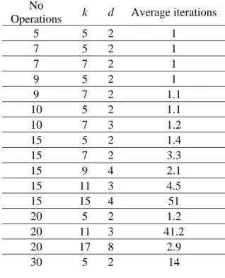
We executed the program for at most 20 iterations where in many instances the convergence factor didn’t exceed its limit and collected the information. For the problems with smaller number of operations, the objective value of the jobs is equal to LB, as Table 5.1 shows. For larger size instances, the results are good enough by considering the fact that only 20 iterations were executed. The second set of instances are the ones that have special structure and their objective function are equal to k d/ , where kanddare two positive integers, from the following definition:

Definition 5.1. For two integers1≤d ≤k, a

(

k

,

d

)

coloring of a graph G is a coloring of the vertices of G with colors

{

0

,

1

,...,

k

−

1

}

such that,

( , )x y ∈E G( )⇒ ≤d c x( )−c y( ) ≤ −k d

The circular chromatic number is defined as

( )

inf{ /

:

c

G

k d G

χ

=

has a

( , )

k d

coloring}

Let an integer from set

{0,1,...,

k

−

1}

be assigned to each vertex of the set of vertices V and also an edge between two vertices of

o

iand

o

j be connected. If

( )

_i

(

_j

)

d

≤

I o

−

I o

≤ −

k

d

where

I V

:

→

{0,1,...,

k

−

1}

, then O is the total number of operations,

V

= =

O

{ ,...,

o

₁

o

_O

}

.

Let the number of operations of a job be n. For

k

≤

n

,

we assign an integer which is i−1 to each operation

o

i of

{ ,...,

o

1

o

k

}

. The remaining operations are assigned randomly. Thus, the vertices of this graph are marked by the colors of

{0,1,...,

k

−

1}

. The edges are assigned as described by Definition 5.1.

We examine the efficiency of our algorithm by solving these instances. Each problem is solved 10 times. The average number of iterations to reach the optimal solution is shown in Table 5.2. 6. CONCLUSIONS

In this paper we have introduced a generalized cyclic open shop scheduling (GCOSS) problem which is a NP-hard problem. To solve this problem, a hybrid algorithm of ACO, Beam search and LP was developed. We generated two types of instances of GCOSS problems and solved them by this method. It was shown that this algorithm works reasonably well by comparing the objective value of these instances to the similar values obtained by an exact method or by checking their lower values.

Table 5.1 The results of Beam-ACO-GCOSS for some instances

LB OP OV Instanc LB OP OV Instanc LB OP OV

4×3_0 3 _ 3* 6×7_0 7 7 8 6×9_0 9 _ 9*

4×3_20 5 _ 5* 6×7_20 6 _ 6* 6×9_20 6 _ 6*

4×3_50 3 _ 3* 6×7_50 4 _ 4* 6×9_50 7 _ 7*

4×3_80 6 _ 6* 6×7_80 6 _ 6* 6×9_80 10 _ 10*

4×3_100 5 _ 5* 6×7_100 7 7 8 6×9_100 9 9 10

3×5_0 5 _ 5* 3×8_0 6 _ 6* 7×9_0 11 14 14*

3×5_20 5 _ 5* 3×8_20 6 _ 6* 7×9_20 9 10 10*

3×5_50 3 _ 3* 3×8_50 5 _ 5* 7×9_50 10 10 11

3×5_80 5 _ 5* 3×8_80 9 _ 9* 7×9_80 10 12 12*

3×5_100 6 _ 6* 3×8_100 7 _ 7* 7×9_100 13 _ 13*

4×5_0 4 _ 4* 4×8_0 5 _ 5* 8×9_0 9 11 11*

4×5_20 5 _ 5* 4×8_20 6 _ 6* 8×9_20 11 _ 11*

4×5_50 3 _ 3* 4×8_50 6 _ 6* 8×9_50 10 _ 10*

4×5_80 4 _ 4* 4×8_80 6 _ 6* 8×9_80 9 9 10

4×5_100 4 _ 4* 4×8_100 6 _ 6* 8×9_100 10 11 11*

3×6_0 6 _ 6* 5×8_0 8 10 10* 3×10_0 8 _ 8*

3×6_20 5 _ 5* 5×8_20 8 _ 8* 3×10_20 10 _ 10*

3×6_50 4 _ 4* 5×8_50 6 _ 6* 3×10_50 7 _ 7*

3×6_80 5 _ 5* 5×8_80 7 7 9 3×10_80 10 _ 10*

3×6_100 7 _ 7* 5×8_100 9 10 10* 3×10_10

0

9 _ 9*

4×6_0 5 _ 5* 6×8_0 7 8 9 5×10_0 8 9 9*

4×6_20 4 _ 4* 6×8_20 7 _ 7* 5×10_20 8 8 9

4×6_50 3 _ 3* 6×8_50 6 _ 6* 5×10_50 7 8

4×6_80 5 _ 5* 6×8_80 7 _ 7* 5×10_80 9 _ 9*

4×6_100 5 _ 5* 6×8_100 9 _ 9* 5×10_10

0

12 13

5×6_0 8 9 9* 7×8_0 11 12 12* 7×10_0 13 14

5×6_20 8 _ 8* 7×8_20 7 9 9* 7×10_20 9 11

5×6_50 5 _ 5* 7×8_50 8 _ 8* 7×10_50 11 12

5×6_80 5 _ 5* 7×8_80 11 12 12* 7×10_80 13 14

5×6_100 6 6 7 7×8_100 12 13 13* 7×10_10

0

13 15

3×7_0 6 _ 6* 3×9_0 7 _ 7* 9×10_0 14 20

3×7_20 8 _ 8* 3×9_20 7 _ 7* 9×10_20 12 14

3×7_50 5 _ 5* 3×9_50 6 _ 6* 9×10_50 10 13

3×7_80 7 _ 7* 3×9_80 7 _ 7* 9×10_80 12 17

3×7_100 7 _ 7* 3×9_100 8 _ 8* 9×10_10

0

16 20.971

4×7_0 6 _ 6* 4×9_0 7 _ 7* 3×15_0 13 14

4×7_20 6 _ 6* 4×9_20 6 _ 6* 3×15_20 11 _ 11*

Instance LB OP OV Instance LB OP OV Instance LB OP OV

4×7_50 6 _ 6* 4×9_50 7 _ 7* 3×15_50 12 _ 12*

4×7_80 6 _ 6* 4×9_80 6 _ 6* 3×15_80 10 _ 10*

4×7_100 6 _ 6* 4×9_100 8 _ 8* 3×15_10

Table 5.1 (Continued)

S L O OV Instan L O OV Instan L O OV

5×7_0 7 8 9 5×9_0 8 9 9* 5×15_0 15 17

5×7_20 6 _ 6* 5×9_20 7 _ 7* 5×15_20 13 _ 13*

5×7_50 5 _ 5* 5×9_50 7 _ 7* 5×15_50 12 _ 12*

5×7_80 6 7 5×9_80 8 8 9 5×15_80 15 15.9805*

5×7_100 8 8 9 5×9_1 9 10 11 5×15_ 18 18.9642* 8×15_0 14 19.9 3×20_ 14 _ 14* 3×25_ 21 22 8×15_20 14 16.9 3×20_ 14 _ 14* 3×25_ 20 21 8×15_50 12 17.9 3×20_ 14 15.9 3×25_ 19 21 8×15_80 14 16.9 3×20_ 15 _ 15* 3×25_ 17 _ 17* 8×15_100 15 19.9 3×20_ 16 _ 16* 3×25_ 23 22.9673* 5×20_20 18 19 3×40_ 29 31 3×30_ 22 24 5×20_50 18 _ 17.9 5×20_ 21 24 3×30_ 27 29 5×20_80 20 23.9 3×30_ 33 _ 33* 3×30_ 22 24

Table 5.2 The average number of iterations to reach the optimal solution in 10 executions

No

Operations k d Average iterations

5 5 2 1

7 5 2 1

7 7 2 1

9 5 2 1

9 7 2 1.1

10 5 2 1.1

10 7 3 1.2

15 5 2 1.4

15 7 2 3.3

15 9 4 2.1

15 11 3 4.5

15 15 4 51

20 5 2 1.2

20 11 3 41.2

20 17 8 2.9

30 5 2 14

REFERENCES

[1] Blum C. (2005), Beam-ACO-Hybridizing ant colony optimization with beam search: an application to open shop scheduling; Computers and Operations Research 32; 1565-1591.

[2] Deuber W., Zhu X. (1997), Circular Coloring of Weighted Graphs; Journal of Graph Theory 23; 365-376.

[3] Dorigo M., Stutzle T. (2004), Ant colony optimization; Boston, MA: MIT Press.

[4] Garey M.R., Johnson D.S. (1979), Computers and intractability; A guide to the theory of NP-Completeness, Freeman, San Francisco.

[5] Kubale M., Nadolski A. (2005), Chromatic scheduling in a cyclic open shop; European Journal of Operation Research; 164(99); 585-591.

[6] Liaw C.F. (2003), An efficient tabu search approach for the two-machine preemptive open shop scheduling; computers & Operations Research 30, 2081-2095.

[7] Ow P.S., Morton T.E. (1988), Filtered beam search in scheduling; International Journal of Production Research 26; 297-307.

[8] Stutzle T, Hoos H.H. (2000), MAX-MIN ant system; Future Generation Computer Systems 16(8); 889-914.

[9] Zhu X. (1992), Star-chromatic numbers and products of graphs; Journal of Graph Theory 16; 557-569.