18
A multi-objective optimization model for process targeting
Mohammad Saber Fallah Nezhad1*, Mehdi Abbasi1, Ehsan Shahin11
Department of Industrial Engineering, Yazd University, Yazd, Iran
[email protected], [email protected], [email protected]
Abstract
Customers and consumers are the necessities for the survival of industries and organizations. Trying to improve the process in order to increase consumer satisfaction is the most important aim of companies. The survival of an organization depends on its ability to continue the activities in compliance with the demands of customers to meet their legitimate needs. An organization is successful when it exactly knows these needs and provides the right products. The selection of the optimal process target is an important problem in production planning and quality control. For complex manufacturing systems, process or product optimization can be instrumental in achieving a significant economic advantage. To reduce costs associated with product non-conformance or excessive waste, engineers often identify the most critical quality characteristics and then use methods to obtain their ideal parameter settings. The purpose of this study is to find the optimum targeting value. a product with two quality characteristics with independent distributions is considered. To determine the market of product sales, random sample size of lot size selected. based on the quality of products, the lot placed in primary market, secondary market, reworked and scraped. To obtain the optimum targeting value, NSGA-II algorithm is used to maximize expected profit and minimize expected loss.
Keywords:Quality control,process adjustment, loss function, profit.
1- Introduction
Customers and consumers are the necessities for the survival of industries and organizations. Trying to improve the process in order to increase consumer satisfaction is the most important aim. The survival of an organization depends on its ability to continue the activities in compliance with the demands of customers to meet their legitimate needs. An organization is successful when it exactly knows these needs and provides the right products.
*Corresponding author
ISSN: 1735-8272, Copyright c 2017 JISE. All rights reserved
Journal of Industrial and Systems Engineering Vol. 10, No. 1, pp 18-34
19
With the complex production system, optimization of the product or process is essential to achieve significant economic benefits (Goethals and Cho, 2012) due to the variations of raw material, labor, production, the quality characteristics of the products may differ from process target (Lee et al.,2007).
To reduce the costs associated with non-conforming products or rework, engineers identify the tolerances limits important parameters and then use statistics methods to obtain the ideal setting for the process parameters. The optimal process adjustment is a statistical method which the optimal settings are determined based on the balance between different types of costs (Goethals and Cho, 2012) .Although the final quality of the product causes the consumer satisfaction by adjusting the process parameters at high values, but raw material and production costs to maintain this level of quality is very expensive. In contrast, when the manufacturers sets the parameters at low levels to avoid the high costs of production, it leads to consumer dissatisfaction (Shao et al., 2000) In a production environment, each product exposes to several stages of process with different operations. There are some variations in final products due to inherent variability and technology of mechanical and chemical processes. Regardless of which process is well designed, usually there are defects in the final product (Duffuaa and El-Ga’aly, 2013). These changes occur due to small random changes that are usually unavoidable to eliminate but the quality control can lower these changes and consequently cause better quality (Noorossana, 2006).The parameters which cause change in the process output may be controlled or uncontrolled, the customer wants a high quality product. So, these factors should be controlled as much as possible in order to meet consumer demands. In theory and in practice, Statistical quality control presents different tools to reduce defects in production process output.
When two quality characteristics exists in the production process then it is important to determine the optimal mean value of each quality characteristic for process adjustment and setting. Also we encounter with three types of produces in such processes: are 1. conforming products 2. semi-conforming products 3. non-conforming products thus we need to apply a trinomial distribution for evaluating the required probabilities. Also since the quality of lot may differ thus we can select different type of markets for selling the products. Hence the objective of this research is to develop a multi-objective optimization model for introduced manufacturing system so that we can determine the optimal setting for each quality characteristic.
The contribution of this research is to develop an economic model for process adjustment based on following assumptions:
• Two quality characteristics existed and the mean value of each one should be optimized. • Two different markets are available for solving the products and the lots with poor quality are
reworked.
• There type of products may be produced that are 1. conforming product 2. semi-conforming product 3. non-conforming product.
• The probabilities of each decision have been determined using a trinomial distribution.
• The objectives of profit and loss have been considered in the model and they are optimized simultaneously.
An organization may need to maximize, profit and customer satisfaction. maximizing profit is important to increase return on investment for the shareholders. Maximizing customer satisfaction will ensure the long term viability of the organization. If the two objectives functions are summarized in one objective, the tradeoff among these objectives will be lumped together. A multi-objective optimization model provides different Insights from a single objective optimization model since the optimization is conducted in multi dimensions showing clearly the tradeoffs among the different objectives. The optimization of multi-objective is different than a single objective and it is known as Pareto optimality where all the efficient or non-dominated points are usually enumerated. The set of efficient points provide decision makers alternatives to select from.
20 1-1- Quality control
Different definitions are provided for quality control. Juran and Godfrey (1999) defines quality control as a group of factors that establish the standards and the quality factors for their application. Ishikawa(1986) defines that quality means the design, manufacture, and supply high quality goods that will satisfy the customer economically and productively. In general, quality control can be decided divided two parts; statistical and non- statistical quality control. Non- statistical methods mostly find the causes of quality problems and offer solutions for the problems, while statistical quality control attempts to match the quality characteristics of manufactured goods with specified standard requirement. Using the statistical methods results in control and inspect the goods with more precision and less costs, on the other hand it leads to limit quality characteristics to fall within defined interval. In general, the purpose of statistical control method is to remove the variability of the process (Noorossana,2006) and (Tareghian and Bozorgnia,1998). determining the optimal features of the product quality is a part of the statistical quality control.
1-2- Determination of optimal process mean
Determining the optimal process mean is one of the economical problems in quality control subject that is a difficult issue to decide in manufacturing processes. Manufacturers usually define limited intervals for the values of quality characteristics ( weight, volume, density) of the products so that the items with quality characteristics within these intervals are categorized as conforming and those that are not within these intervals are categories ones which will be sold in a lower cost or returned to the production process for rework (Darwish et al., 2013). Generally, the process mean is effective on the expected total profit, nonconforming parts, inspection and rework costs (Chen and Lai, 2007). So the determination of optimal mean, is based on a balance between cost of production, benefits of conforming items, and costs associated with nonconforming products (Park et al., 2011).
1-3- Literature
The first model for optimal target was presented by Springer (1951). This model was considered to determine the process mean of as nonconforming processes with the aim of lowering total costs of production. The quality characteristics presented in this model followed mean gamma distribution. Bette presented another model for this purpose. In Bette's model, the optimal process mean is determined by consisting the upper and lower limits. The main problem of this model, was not presenting an exact method for determining the optimal values (Pulak et al., 1996) inspired by Springer's model, Hunter and Kartha(1977) presented a model which maximize the total revenue by determining the optimal process mean. In this model, the process has a lower limit so that if the characteristics of product quality is more than this limit, then it is categorized for primary market and if it is less than the limit, it is sold with a lower price ( fixed price) in a secondary market (Das,1995). To determine the rejection or acceptance of the products, quality variables will be inspected first. In this model it is assumed that the quality variable are normally distributed. Finally, by maximizing the expect benefit, which includes the sale price, cost of production, rework, inspection, and other quality costs; optimal value of mean and tolerance limits are achieved. Chung et al presented the industrial process control model for filling cans to extend Lee’s model. this model assumes high correlation between quality and functional variables. By using the single-step method, the aims are to minimize the expected total cost for obtain the optimal mean value and limits (Chen, 2009). Based on empirical analysis, Geothals et al.(2012) developed a method to determine the optimal mean value. More predictability of optimal mean value in variable process condition is the most important advantage of this method (Goethals, 2012). Darwish et al. (2013) claim that the models presented relating to mean inventory are applicable for the fixed demands but not in real world. To overcome this problem, they presented a model which determines the optimal mean value, accumulated amount, and order point considering the fact that the demand is not specified ( Darwish et al., 2013). The most recent work in this area, is the model presented by Duffuaa and Gaaly (2013) in which a multi-objective function with the aim of maximizing profits, income, and conformity of product is used to
21
determine optimal mean. In this model, a lower specification limitation is used to accept or reject the products, so that the products with quality characteristics more than this limit are sold in primary market and those which are less than this limit, in a secondary market (Duffuaa and Gaaly, 2013).
Fallah Nezhad and Shahin (2013) developed a model to maximize expected profit per item of a multi-stage production system by determining best adjustment points of the equipment used based on technical product specifications defined by designer. In this system, the quality characteristics of items produced should be within lower and higher tolerance limits. When a quality characteristic of an item either falls beneath the lower limit or lies above the upper limit, it is reworked or classified as scrap, each with its own cost. A function of the expected profit per item is first presented based on equipment adjustment points. Then, the problem is modeled by a Markovian approach. Finally, numerical examples are solved in order to illustrate the proposed model.
Fallahenzhad and Ahmadi (2014) considered a production system with several quality characteristics. Their paper investigated a single-stage and two-stage production systems where specification limits are designed for inspection. When quality characteristics fall below a lower specification limit (LSL) or above an upper specification limit (USL), a decision is made to scrap or rework the item. The purpose was to determine the optimum mean for a process based on rework or scrap costs. In contrast to previous studies, costs are not assumed to be constant. In addition, their paper provided a Markovian model for multivariate Normal process. Numerical examples were performed to illustrate the application of the proposed method.
All work done in this area, uses one variable as quality characteristics. But in real world, products are in a multi- dimensional quality. Customers examine the products with considering more than one quality characteristics. This study aims to provide a model which is closer to practical applications for such issues. For this purpose, the model will be developed with considering two quality characteristics. In order to solve the proposed model, the method of NSGA II is applied to rank the set of Pareto optimal solutions using standard deviation of the obtained values.
1- 4 - NSGA algorithm
NSGA algorithm was first proposed by Srinivas and Deb (1994). In the case of the problems with multiple objective functions genetic algorithm should be redefined and extended due to high computational complexity and lack of standards that is named as NSGA, Deb et al (2002) introduced the second version of the algorithm named NSGA II. In general, components of the NSGA II algorithm is as follows:
1- 4 - 1- Chromosome
Chromosome in the genetic algorithm represents the solutions of to the problem while each chromosome consists of a number of genes. correct election of the chromosomes has a great impact on the computational time. Overly, the chromosomes should be selected so that it contains the data to solve the problem in addition to its simplicity (Ebrahimizade, 2013). In this study, each Chromosome is considered as the mean value for the process, that is a real number.
1- 4- 2- population
A set of chromosomes, constitutes a population. Then using the operational algorithm for related population by changing the structure and the members of new generation, the new population is obtained (Sadeghie, 2006). showed the number of each population.
1- 4- 3 crossword function
In this function, two members of the population are considered as a parent and then by switching the genes of two parents, a new member will be generated. The purpose of this section is to generated a new member so that the new member has a combination of characteristics of both parents. Intersection operators include one-point crossover, two-point crossover, uniform crossover, and Heuristic crossover.
22
Due to the structure of the chromosomes for crossover operator, Heuristic crossover method is used in this model. The structure of this type of crossover operator is so that if both parents are 12 22 2
2
( , , , n)
x = x x … x And 11 12 1 1
( , , , n)
x = x x … x , then the child y=(y y1, 2,…,yn) is as denoted in equation (1):
) 1 (
(
2 1)
2i i i i
y =u x −x +x
In which, u is a random number in the interval [1,0]. In order to determine the number of solutions obtained from the intersection operator, a constant number named intersection rate is used (Sadeghie, 2006) and (Deep, 2007).
1- 4- 1- Mutation
This operator selects a gene on chromosome randomly and then considering the nature of the chromosome, necessary changes are applied to the genes. In the binary encoding, the mutation operator causes the selected gene changes to zero if its value is one, and changes to one if the value is zero. Gaussian mutation is another form of mutation operator for real encoding. In this method, mutation is calculated using equation (2):
) 2 (
( )
'0,1
i i
x
= +
x
N
In this regard, xi' is the mutated value of point xi in solution population of the problem. N ( 0,1) is a random number from a standard normal distribution. Rate of mutation is a constant number which expresses the probability of mutation for each Chromosome and is shown by pm (Sadeghie, 2006) and (Gong, 2010). In this study, Gaussian mutation operator is used in order to the real encoding of chromosomes.
1- 4- 5 - General Process of the NSGA II Algorithm
To start the proposed algorithm, the chromosomes should be encoded by the conventional methods in genetic algorithm. The encoding method is considered for the real numbers in the proposed structure, so that a random number is allocated to each chromosome in a specified range for that variable. After generating the random initial population, the members of the population are ranked in several categories based on the Dominate principal. Then, all obtained results are compared against each other. After comparison, the collection of solutions which is better than other results with regards to the objective function are placed in the first category. By removing the effect of the elements in the first category on other results are placed in the second category, third and so on and we continue until all the solutions are placed in a category. This process is continued in any stage of the algorithm until the results collection of the first front is the nearest value with the optimum (Deb et.al, 2002) and (Srinivas and Deb, 1994). After fronting the generated population, congestion gap Congestion is used for ranking of the front members. In order to calculate the distance gap in each front, the front members are arranged based on the target function of the problem. Extreme value is considered for the results with the lowest and highest value. Then using the equation (3), congestion gap for the target function k is calculated. Congestion gap for the midpoints are calculated by the summation of the target function congestion gap using equation (4).
) 3 ( [ ]
( )
( )
[ 1, ]( )
[ 1, ],
k i k k i k
k i k max min
k k
z
x
z
x
cd
x
z
z
+
−
−=
−
) 4 (
( )
k( )
k
23
[ ]i k,
x is the answer i from the target function k, zk( )x is amount of the target function k in point x,
max k
z is maximum of the target function k zkmin is minimum of the target function k (Srinivas and Deb, 1994).
Selection of a parent in each generation of solution is done by applying binary tournament with a c pop
p n number. In binary tournament method, two members are selected from the population randomly and arranged based on the category and congestion gap. The best arranged member is elected as the first parent. This process will be repeated for the second parent. By repeating the binary operator on the population of each generation, a collection with p nc popmembers of that generation is selected for the crossover. After crossover, a number of p nm p po members of the population is selected randomly and mutation is applied for them. So, a new population of children and mutants is created. In future, this population will be integrated with the main population. The population consists of the children, mutants, and the current population and they are sorted based on a descending order of congestion gap, then based on an ascending order of their rank. The number of members in the next population are chosen equal to the number of members in the main (primary) population ،while the other members are discarded based on the sorted new population. This process is continued to meet the end conditions. A collection of the solutions are presented as the Pareto optimal solution when the algorithm ended. Each of this collection members could be an optimal solution depending on decision making condition (Deb et.al, 2002) and (Srinivas and Deb, 1994).
1- 4- 6 - Ranking the collection of Pareto optimal solution
After determining the optimal category, the following steps should be done for sorting the collection of the Pareto optimal solution:
1. First, each function should be optimized individually. The optimal solution for the first function is T1 and for the second function is T2 ,.
2. Si could be calculated for each obtained solution:
)
5
(
( )
( )
2' 1
k i i
k k i
f T
S
f T
=
=
∑
3. Deviation of optimal solutions is calculated through the equation (6) as:
)
6
(
100 2 1, 2, ,
2
i i
S
i= … n PAD = −
4. The collection of the Pareto optimal solution is sorted from small to large according to PADivalues. In this case, the results with less PADivalues are more appropriate.
2- Problem solving
Consider a product which has two quality characteristics where each of them has a lower specification limit. The first quality characteristic X1 follows a normal distribution with unknown mean,
µ
1, standard deviation,σ
1, and has a lower specification limit of LSL1, and the second quality characteristic X2a normal distribution with unknown mean,µ
2, standard deviation,σ
2, and has a lower specification limit of LSL2. However, a product will be conforming if both of quality characteristics are more than their24
lower specification limits,(X1≥LSL X1, 2 ≥LSL2). If one of the characteristics is more than its lower specification limit and the other characteristic is less than its lower specification limit,
1 1 2 2
(X ≥LSL X, <LSL ) or (X1<LSL X1, 2≥LSL2),then this product is called semi conforming; and if
both quality characteristics are less than specification limits then it will be categorized as nonconforming. The products are produced in a lot of size N. Sampling plan is used for the determination of the lot quality. The applied sampling plan is as follows:
A sample of size n from a lot of size N is selected randomly. The sample is inspected and the decision is made on the quality of lot based on the number of nonconforming (D) and semi-conforming (D1) items.
1
d and d2 (d1<d2) are two acceptance limits for the number of nonconforming items, while d3 and d4
(d3<d4) are those for the number of semi-conforming items. First, if the numbers of the nonconforming items are less than d1 and the numbers of the semi-conforming items are less than d3,then the lot is sold in a primary market at a specified price a for each item. In second case, if the numbers of the nonconforming items are more than d2, and the numbers of the semi-conforming items are more than d4
then the lot will be %100 inspected, so that the conforming products will be sold in the primary market, while the rest of them with a specified cost
s
for each item becomes scrapped. In the third case, if1 2 1 3
(d < ≤D d , 0≤D ≤d )or (D≤d d2, 3<D1≤d4), then the lot at price of
r
for each product(r<a)will be sold in the secondary market. In the other cases, the lot at price R for each item will be reworked. It is assumed that the rework operation is not complete and the reworked lot is about to place in each of the groups of the primary market, the secondary market, the reworked items, or the scrapped items.
2- 1- Notations 1
C and C2: production cost per unit of the first and second quality characteristics
i: inspection cost per unit of products
n: sample size
N: lot size
D: numbers of nonconforming products in a sample of size n
1
D: numbers of semi-conforming products in a sample of size n
1, 2, 3, 4
d d d d : inspection limit, for the number of nonconforming and semi-conforming production in
sample 1
LSL: lower specification limit for the first quality characteristics 2
LSL : Lower specification limit for the second quality characteristics
a: sale price of the product in the primary market
25
S: cost of scrapped product 1, 2
g g : cost of one unit of excess material in the product for the first and second quality characteristics
R: reworking cost 1
K : coefficient of quality loss function in the primary market 2
K : coefficient of quality loss function coefficient in the secondary market 2-2- Assumptions
To model the problem, the following assumptions are considered:
1. The lot size is large enough to apply the trinomial distribution as a probability distribution of the number of nonconforming and semi-conforming items.
2. Process cost is directly proportional to the mean value of the quality characteristics.
3. There is no shift and change in the process target and the process is under statistical control. 2- 3- fundamental relations
The probability of producing a nonconforming product is:
) 7 ( 2 2 2
1 1 12 2
2 1
1
1 ( )
( ) 2
2
1 1 1 2 2 1 2
1 2
1 1
(X , LSL )
2 2
x
LSL x LSL
m p LSL X
e
dx e dxµ σ
µ
σ
σ
π
σ
π
−
− −
−
−∞ −∞
=
<
<
=∫
∫
The probability of producing a semi-conforming product is:
) 8 ( 2 2 2
1 1 12
2 1
2 2 2 1 12
2 1 2 2 1 1
1 ( )
( ) 2
2
2
1 2
1
1 ( )
( ) 2
2 2 1 2 1 1 U 1 1 2 2 1 1 2 2
2 1 1 2 2 1 1 2 2
x LSL LSL x LSL LSL
m = p((X < LSL , X LSL ) (X LSL , X < LSL )) =
x e dx x e dx dx dx
e
e
µ σ µ σ µ σσ π σ π
µ σ
σ π σ π
− − ∞ − − −∞ − − ∞ − − −∞ ≥ ≥ +
∫
∫
∫
∫
According to equation (8), the probability of a product to be nonconforming in the first quality characteristics and conforming in the second quality characteristics could be obtained from equation (9); and the probability of a product to be nonconforming in the second quality characteristics and conforming in the first quality characteristics could be obtained from equation (10) as follows:
) 9 ( 2 2 2 1 12
2 1
1
2
1
1 ( )
( ) 2
2 2 1 2 ' 2 1 1 1 2 2 x LSL LSL x e dx
m
e
dx
µ σ
µ
σ
σ
π
σ
π
− − ∞ − − −∞
=
∫
∫
) 10 ( 2 2 2 1 122 1
1
2 1
1 ( )
( ) 2
2 2 1 2 '' 2 1 1 1 2 2 x LSL LSL x e dx
m
e
dx
µ σ
µ
σ
σ
π
σ
π
− − ∞ − − −∞
=
∫
∫
The probability of producing a conforming product is as following:
)
11
(
3 1 2
m =1-m -m
26
The probability distribution of the number of nonconforming and semi-conforming items is obtained from the trinomial distribution with the parameters m1,m2 and m3. In the first case, the product is sold in the primary market, If the number of the nonconforming products is less than d1 and the number of semi-conforming items is less than d3, the probability of this case is as follows:
)
12
(
(
)
1 3(
)
( )
1 1 1 3
0 3 1 2 0 ! , ! ! ! d d i i j
j n i j
n
p p D d D d m m m
i j n i j
− − = = = ≤ ≤ = − −
∑∑
If the number of nonconforming products is more than d2 and the number of semi-conforming products is more than d4, then the lot is considered as scrapped, where the probability of this case is as following:
) 13 (
(
)
(
)
2 4 ( )2 2 1 4 1 2
1 3 1 ! , ! ! !
n n i
i n i j
i d j
j
d
n
p p D d D d m m
i j n i j m
−
− − = + = +
= > > =
− −
∑ ∑
If (D≤d d2, 3<D1≤d4)or (d1< ≤D d2, 0≤D1≤d3), then the lot could be sold in a secondary market with the probability ofp3 as follows:
) 14 (
(
) (
)
(
)
(
)
2 4 3 2 3 13 2 3 1 4 2 1
( ) 1 2 0 ( ) 1 2 3 1 0 1 1 3 3
, , 0
! ! ! ! ! ! ! ! + d d
i n i j
i j d
d d
i n i j
i
j
j
d j
p p D d d D d p d D d D d
n
m m i j n i j
n
m m i j n i j
m m − − = = − − = = + +
= ≤ < < ≤ ≤ =
− − − − ≤ + ≤
∑ ∑
∑ ∑
In the other cases, the lot is reworked. The probability of reworking the lot is:
)
15
(
4
1
1 2 3p
= − − −
p
p
p
we need to determine the conditional expected value of quality characteristics for evaluating give-away cost of excess materialy , is the conditional expected value of the quality characteristics 1' x1, conditioned on the event that x1is more than LSL1.
) 16 (
(
)
1 12 1
1 12 1 1 1 1 ( ) 2 1 1 ( ) 2 1 1 '
1 1 1 1
1 1 1 2 1 2 LSL LSL x x x
y E x x
dx LSL dx
e
e
µ σ σ π µ σ σ π ∞ ∞ − − − − = ≥ =∫
∫
' 2y is also the conditional expected value of the quality characteristicsx2, conditioned on the event that 2
27 ) 17 (
(
)
2 22 2
2 22 2 2 2 1 ( ) 2 2 2 1 ( ) 2 2 '
2 2 2 2
2 2 1 2 1 2 LSL LSL x x x
y E x x
dx LSL dx
e
e
µ σ σ π µ σ σ π ∞ ∞ − − − − = ≥ =∫
∫
2- 4 - Profit objective function
Profit objective function is determined as the equation (18). It consists of benefit from sale in the primary market (equation 18, part I), the benefit of the scrapped items (equation 18, part II), benefit from the sale in the secondary market (equation 18, part III), and benefit from the reworked items ( equation 18, part IV). ) 18 (
(
)
(
) (
)
( )
2 3 1 4 2 1 31 1 2 2 1 1 3
1 1 2 2 3 2 1 4
1 1 2 2 , 1 ,0
( ,
,
&
)
3
D d d D d d D d D d
aN in c N c N D d D d
iN c N c N m Na (1-m )NS D d D d
rN in c N c N
PN
E PN in
µ
µ
µ
µ
µ
µ
≤ < < ≤ ≤− − − ≤ ≤
− − − + − > >
− − =
− −
≤ ≤
−RN ow.
Part I of equation (18) has fallowing terms: income of the total sale is multiplied with its price , aN , minus the inspection cost of a random sample (in), minus the production cost of the all products,
1 1 2 2
(cµ N+c µ N).
The second part of equation (18) denotes the benefit of the items that are considered as scrapped. In this case, the lot is %100 inspected. The conforming products are sold in the primary market and the rest are considered as scrapped. In such conditions, the benefit of this case is equal to the income from the sale of the conforming products in the primary market, (m Na , minus the inspection cost of all items, (3 ) iN), minus the cost of production, (c1µ1N +c2µ2N), minus the cost of the products which are considered as scrapped, ( 1( −m NS3) ).
The benefit from the items that are sold in a secondary market is obtained in the third part of equation (18). The benefit in this case equals to: the income from the sale of items in the secondary market (rN), minus the cost of sample inspection (in), minus the production cost of all products (c1µ1N +c2µ2N). The forth part of equation (18) considers the benefit of reworked items. In this case, we have assumed that the reworking process is not complete and the lot may be placed in each of mentioned pasts again; so that the benefit in this case is equal to the expected value of total profit ( (E PN)), minus the cost of inspecting the sample (in), minus the reworking cost (RN).
According to the profit function, the expected value of profit can be obtained from equation (19) as follows: ) 19 (
( )
( )
1 1 1 1 1 2 2 1
2 1 1 2 2 2 2 3 2 3 2
3 3 1 1 3 2 2 3
4 4 4
(1
)
E PN
aNp
inp
c
Np
c
Np
iNp
c
Np
c
Np
m Nap
m NSp
rNp
inp
c
Np
c
Np
E PN p
inp
RNp
µ
µ
µ
µ
µ
µ
=
−
−
−
−
−
−
+
− −
+
−
−
−
+
−
−
28
)
20
(
( )
1 1 2 3 2 3 2 34
3 4 4 1 1 1 2 3 2 2 1 2 3
1
E PN = ( )(aNp - inp - iNp + m Nap (1 - m )NSp + rNp 1 - p
-inp - inp - RNp - c µ N(p + p + p ) - c µ N(p + p + p )) −
By dividing the equation (20) to N , the expected value of profit per unit of the product is obtained as following: ) 21 (
( )
1 1 2 3 2 3 2 3 34
4 4 1 1 1 2 3 2 2 1 2 3
1 n n
E P = ( )(ap - i p - ip m ap (1 - m )Sp + rp - i p
-1 - p N N
n
-i p - Rp - c (p + p + p ) - c (p + p + p ))
N
µ
µ
+ −
2- 5 - loss function
Both quality characteristics in this study, do not have upper specification limit, thus the larger- the better loss function is used for quantifying consumer loss. It is obvious that consumers becomes more satisfied when the values of quality characteristic increase (Duffuaa and Gaaly, 2013).Taguchi loss equation in this case is as follows:
) 22 ( 2 1 (X) L k X =
Where k , is the coefficient of quality loss function.
In this study, according to market segmentation, loss function is as follows:
) 23 ( '' 3 2 ' 3 2
1 1 3
2
3 2 3
3 3 ( ) 1 , , ( ) 1 '
1 1 1
'
2 2 2
'
1 1 1 1
'
2 2 2
k NL +
(m m )Ng (y - LSL )+
(m m )Ng (y - LSL )
k m NL + m Ng (y - LSL )+
LN = m Ng (y - L
D d D d
D d
SL ) m Na D
≤ + + ≤ > + −
(
)
(
)
(
)
2 12 3 1 4
3 2 1 '' 3 2 ' 3 2 1 4
1 , 0
, ( ) ( ) & '
1 1 1
'
2 2 2
d D d D d
D d d D d
k NL +
(m m )Ng (y - LSL )+
(m m )Ng (y - LSL ) a
E
d
r N L
< ≤ ≤ ≤ < ≤ + + + − ≤ >
.o w
In which, L1 is the Taguchi loss function of products sold in the markets.
) 24 ( 2 2 2 1 12
2 1
1
1 ( )
( ) 2
2
1 2 1 2 2
1 1 2 2
1 1 1 1
2 2
x
x
L dx e dx
x
e
xµ σ
µ
σ
σ
π
σ
π
− − ∞ ∞ − − −∞ −∞ =
∫
∫
29
)
25
(
2 2 2 1 12
2 1
1 2
1
1 ( )
( ) 2
2
2 2 1 2 2
1 1 2 2
1 1 1 1
2 2
x
LSL LSL
x
L dx e dx
x
e
xµ σ
µ
σ
σ
π
σ
π
− −
∞ ∞ −
−
=
∫
∫
)
26
(
(
) (
)
3 E x1 LSL1 2 2
m = loss ≥ E loss x ≥LSL
1 1
(k NL )is total loss of sold items in the first market. And
(
'')
'3 2 1( 1 1)
m +m Ng y −LSL , is the expected give-away cost of the first quality characteristics; and
(
m3+m2')
Ng2(y2' −LSL2) is that of the second quality characteristics.In the second part of the equation (23), after implementing %100 inspection plan, a part of the lot is conforming and could be sold in the primary market. In this case, Taguchi loss function of such products is (K m NL1 3 2), also the expected the lost income value due to lack of sale in the primary market is(1−m Na3) , and give-away cost of the excess material used in the products are considered as loss
where '
3 1 1 1
(m Ng y( −LSL)), is the expected give-away cost of excess material for the first quality characteristics and
( )
m3 Ng2(y2' −LSL2), is the second quality characteristics.(k NL2 1)is total loss of sold items in the secondary market. Also in this case, ((a−r N) ) is the difference between selling prices in the primary and secondary market considered as the loss value and
(
'')
'3 2 1( 1 1)
m +m Ng y −LSL is the expected give-away cost for the first quality characteristics and the expected give-away for the second quality characteristics, is
(
m3+m2')
Ng2(y2' −LSL2).In the fourth part which the process is reworked, then the lot may be placed again in one of the explained parts. To this purpose, the loss is considered as expected value of total loss.
The total expected value of loss for the lot is as following:
)
27
(
'' ' '
3 2 3 2
1 2 3 3 2
'' ' '
3 2 3 2
) '
1 1 1 1 1 1 1 2 2 2 1
' '
3 2 1 1 1 2 2 2 2 2 3 2 1 3
'
1 1 1 3 2 2 2 3 3 4
E(LN) = k (NL p + (m m )Ng (y - LSL )p + (m m )Ng (y - LSL )p +
k m NL p + m Ng (y - LSL )p + m Ng (y - LSL )p + (1 - m )Nap k (NL p )+
(m m )Ng (y - LSL )p + (m m )Ng (y - LSL )p + (a - r)Np +E(LN)p
+ +
+
+ + +
Equation (27) is arranged as equation (28) :
)
28
(
''
3 2
4 '
3 2 1 2 3
3 2
'' ' '
3 2 3 2
1
( )
1
)
'
1 1 1 1 1 1 1
' '
2 2 2 1 3 2 1 1 1 2
'
2 2 2 2 3 2 1 3
'
1 1 1 3 2 2 2 3 3
E(LN)= k (NL p )+(m m )Ng (y - LSL )p +
p
(m m )Ng (y - LSL )p + k m NL p + m Ng (y - LSL )p
+m Ng (y - LSL )p +(1 - m )Nap k (NL p )+
(m m )Ng (y - LSL )p +(m m )Ng (y - LSL )p +(a - r)Np
+ −
+
+
+ +
30
)
29
(
''
3 2
4 '
3 2 1 2 3
3 2 2
'' '
3 2 3 2
1
( )
1
)
'
1 1 1 1 1 1 1
' '
2 2 2 1 3 2 1 1 1 2
'
2 2 2 2 3 2 3
' '
1 1 1 3 2 2 2 3 3
E(L)= k (L p )+(m m )g (y - LSL )p +
p
(m m )g (y - LSL )p + k m L p + m g (y - LSL )p
+m g (y - LSL )p +(1- m )ap k (L p )+
(m m )g (y - LSL )p +(m m )g (y - LSL )p +(a - r)p
+ −
+
+
+ +
2-6- solution
In order to solve this model, a search algorithm is developed: Step 1 :
Each target is separately optimized by linear grid search method with Step γ in the interval of
[
]
1 1, 1
I = LSL LSL +B and I2=
[
LSL LSL2, 2+B]
in which, B is a positive number.Step 2:
Optimal Pareto points are created through the following steps:
i.
(
* *)
1 2
min ,
min
T = T T and
(
* *)
1 2
Max ,
Max
T = T T is defined.
ii. Ti =TMin+ ∈iγ [Tmin,Tmax] i=1,...,n and Tj =TMin+jγ∈[Tmin, Tmax] j=1,...,n is defined in which
min
2
2j U j j=1,...,n
U = + γ ,
min
2
2i U i i=1,...,n
U = + γ ,
min
1
1j U j j=1,...,n
U = + γ ,
min
1
1i U i i=1,...,n
U = + γ
iii. In which Ti is considered as the Pareto optimal solution if there is no Tj, so that:
(T ) (T ) : k=1,2
k j fk i
f ≥ Step 3:
The Pareto optimal solution s are ordered as:
i. Normalization: 2 *
(T )
, i=1,...,n k=1,2. (T )
k i
k k
f f
ii. The summation of normalized numbers is defined as:
2
* 1
(T ) (T )
k i
i
k k k
f s
f
=
=
∑
iii. Deviation percent is defined as:
2 2
i i
s
PAD = −
iv. The points are ranked based on PA Di in the order of ascending. The points with lower
i
PA D values are better solutions.
3- Numerical example
In this section, an example is designed and solved by an optimization software to evaluate the proposed model. As the best of author’s knowledge, meta-heuristic methods are not applied for solving the
31
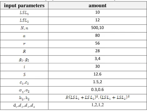
economic models of optimal process adjustment thus we cannot refer to literature for adopting the Genetic algorithm. Consider a company which produces a product with two quality characteristics. The first quality characteristics X1 follows a normal distribution with unknown mean µ1 , standard deviationσ1, lower specification limit of LSL1, and the second quality characteristics X2 of a normal distribution with unknown meanµ2, standard deviationσ2, and lower specification limit of LSL2. The aim is to find the optimal amount of the two quality characteristics by maximizing the expected profit and minimizing the expected loss. The other required information is available in table (1).
Table 1. input parameters of the numerical example
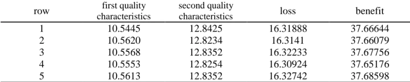
At first, two objective functions of the problem are optimized individually by the numerical grid search method, then objective functions are optimized simultaneously using NSGAII. Optimal solutions of each objective function is presented in table (2), separately. The results show that a maximum profits of %37.77 is obtained by mean value of 10.6 for the first quality characteristics and mean value of 12.9 for the second quality characteristics. Also, the mean value of 10.5 and 12.8 for the first and the second quality characteristics respectively, leads to loss of 16.27. Table (3) shows five optimal Pareto solutions sorted by PAD standard that each of these solutions could be the optimal solutions of the problem according to the decision maker priorities. A solution algorithm is developed in the sub-section 2-6 to order the Pareto optimal solution and we can select the best solution based on this algorithm but we may apply other methods of Multi Objective Decision Making (MODM) that are discussed in the reference (Friedricha and Luibleba , 2016).
Table 2. The optimal mean value of objective functions
expected loss
second quality characteristics
first quality characteristics
expected
benefit
second quality characteristics
first quality characteristics
16.27
12.8
10.5
37.77
10.6
10.6
amount
input parameters
10 12 500,10
80 56 28 3,4 30 12.6 1.5,2 0.3,0.6
1,2,1,2
1 2 3 4
32
Table 3. five optimal Pareto sorted solutions
benefit loss
second quality characteristics
first quality characteristics
row
37.66644
16.31888
12.8425
10.5445
1
37.66079
16.3141
12.8234
10.5620
2
37.67756
16.32233
12.8352
10.5568
3
37.65176
16.30924
12.8254
10.5553
4
37.68598
16.32742
12.8352
10.5613
5
37.35 37.4 37.45 37.5 37.55 37.6 37.65 37.7 37.75 37.8 37.85 16.25
16.3 16.35 16.4 16.45 16.5 16.55 16.6
profit
lo
s
s
objective function
Figure 1. Optimal Pareto solutions
4- Conclusions
Economic adjustment of a process parameters is one of the most important subjects in the statistical process control. Because of deviations occurred due to raw materials, labor, and process conditions, products quality may be different from the target values. Choosing the target values for the nominal mean of the process may lead to minimum production cost but on the other hand, this adjustment may lead to increase the number of nonconforming items. In this research, an optimization model with two objective functions are developed for optimal process adjustment. The results of solving this model indicate that the optimal mean values of the quality characteristics have a small difference from the lower limits which is due to the considered give-away cost for both characteristics. We suggest to consider optimal design of sampling plan and optimal process adjustment with each other in one optimization model to investigate their relation and properties of optimal solutions.
References
Chen, C.-H. and M.-T. Lai, Economic manufacturing quantity, optimum process mean, and economic specification limits setting under the rectifying inspection plan. European Journal of Operational Research, 2007. 183(1): p. 336-344.
Chen, C.-H. and H.-S. Kao, The determination of optimum process mean and screening limits based on quality loss function. Expert Systems with Applications, 2009. 36(3): p. 7332-7335.
33
Darwish, M., F. Abdulmalek, and M. Alkhedher ,Optimal selection of process mean for a stochastic inventory model. European Journal of Operational Research, 2013. 226(3): p. 481-490.
Das, C., Selection and evaluation of most profitable process targets for the control of canning quality. Computers & industrial engineering, 1995. 28(2): p. 259-266.
Deb, K., Pratap, A., Agarwal, S., & Meyarivan, T. A. M. T. (2002). A fast and elitist multiobjective genetic algorithm: NSGA-II. IEEE transactions on evolutionary computation, 6(2), 182-197.
Deep, K. and M. Thakur, A new mutation operator for real coded genetic algorithms. Applied mathematics and Computation, 2007. 193(1): p. 211-230.
Duffuaa, S.O. and A. El-Ga’aly, A multi-objective optimization model for process targeting using sampling plans. Computers & Industrial Engineering, 2013. 64(1 :(p. 309-317.
Ebrahimizade, A. The problem of locating the hub maximum coverage under uncertainty. Master thesis of yazd University , [Persian] 2013.
Fallah Nezhad M.S., Niaki S.T.A. and Shahin E, A Markov Model to Determine Optimal Equipment Adjustment in Multi-stage Production Systems Considering Variable Cost. Iranian Journal of Operations Research, 2013. 4(2): pp. 146-160.
Fallah Nezhad M.S. and Ahmadi E, Optimal Process Adjustment with Considering Variable Costs for Uni-variate and Multi-variate Production Process. International Journal of Engineering, 2014. 27(4): p. 561-572.
Friedricha D. and Luibleba A., Assessment of standard compliance of Central Europeanplastics-based wall cladding using multi-criteria decision making (MCDM). Case Studies in Structural Engineering, 2016. 5: p. 27–37
Goethals, P.L. and B. Cho, The optimal process mean problem: Integrating predictability and profitability into an experimental factor space. Computers & Industrial Engineering, 2012. 62(4): p. 851-869.
Gong, W., Cai, Z., Ling, C. X., & Li, H. (2010). A real-coded biogeography-based optimization with mutation. Applied Mathematics and Computation, 216(9), 2749-2758.
Hunter, W. G., & Kartha, C. P. (1977). Determining the most profitable target value for a production process. Journal of Quality Technology, 9(4), 176-181.
Ishikawa, K. (1986). Guide to quality control. Quality Resources.
Juran, J., & Godfrey, A. B. (1999). Quality handbook. Republished McGraw-Hill.
Lee, M.K., et al., Determination of the optimum target value for a production process with multiple products. International Journal of Production Economics, 2007. 107(1): p. 173-178.
Noorossana. R. Statistical Quality Control. Iran University of Science and Technology. Third Edition, [Persian],2006.
34
Park, T., Kwon, H. M., Hong, S. H., & Lee, M. K. (2011). The optimum common process mean and screening limits for a production process with multiple products. Computers & Industrial Engineering, 60(1), 158-163.
Pulak, M. and K. Al-Sultan, "The optimum targeting for a single filling operation with rectifying inspection". Omega, 1996. 24(6): p. 727-733.
Sadeghie, A. Decision-making based on genetic algorithm optimization. New Science Publications, [Persian] ,2006.
Shao, Y.E., J.W. Fowler, and G.C. Runger, Determining the optimal target for a process with multiple markets and variable holding costs. International Journal of Production Economics, 2000. 65(3): p. 229-242.
Springer, C. H. (1951). A method for determining the most economic position of a process mean. Industrial Quality Control, 8(1), 36-39.
Srinivas, N. and K. Deb, Muiltiobjective optimization using nondominated sorting in genetic algorithms. Evolutionary computation, 1994. 2(3): p. 221-248.
Tareghian H. R., Bozorgnia A., the application of the quality control systems using the statistical methods. Publishers of Ferdowsi Mashhad University,[Persian] 1998 .219.