1
Wave Attenuation in Salt Marshes
By
Katharine Krovetz
Senior Honors Thesis Environmental Science
University of North Carolina at Chapel Hill
December 6th, 2017
Approved:
Johanna Rosman, Advisor
Christine Voss, Reader
2
Abstract
Salt marshes can provide several ecosystem services including shoreline protection. One
of the ways marshes do this is by attenuating waves. However, the rate at which waves are
attenuated by marshes is highly variable. Previous studies have found that the rate of wave
attenuation varies with water depth, vegetation characteristics, bottom profile, and wave
conditions. This study examined how these factors affect wave attenuation rate at four marsh
sites in coastal North Carolina with different vegetation and bottom profile characteristics. The
rate of wave attenuation was found to increase with decreasing water depth and increasing
vegetation height and increasing vegetation density. Sites with short vegetation, which is
submerged more of the time, had larger rates of decrease in wave attenuation with increasing
depth than sites with tall vegetation. Waves with long periods were attenuated less than waves
with short periods. Attenuation rates were much less and decreased more with increasing water
depth during storm conditions than during normal conditions at the same site.
1.
Introduction
Salt marshes provide many benefits to humans, including protection from storms and the
stabilization of shorelines (Barbier et al., 2011). Coastal wetlands are estimated to provide $23.2
billion in storm protection every year in the United States (Constanza et al., 2008). Marshes help
shoreline stabilization by increasing vertical accretion (Morris et al. 2002), reducing erosion, and
increasing the surface elevation of the area (Shepard et al., 2011). One of the ways in which salt
3
Wave attenuation is a well-observed phenomenon in salt marshes whereby wave energy
is decreased over the salt marsh. Wave attenuation is important for protecting the shoreline from
erosion due to wave energy. There are large variations between the findings of studies
investigating how much wave attenuation occurs. One study of Spartina alterniflora in Virginia
marshes found that most wave energy dissipated in the first 2.5 meters, and almost no wave
energy remained at 30 meters (Knutson et al., 1982), while another study in north Norfolk,
England found that wave height reduction was 61% over 180 meters (Möller et al., 2001). The
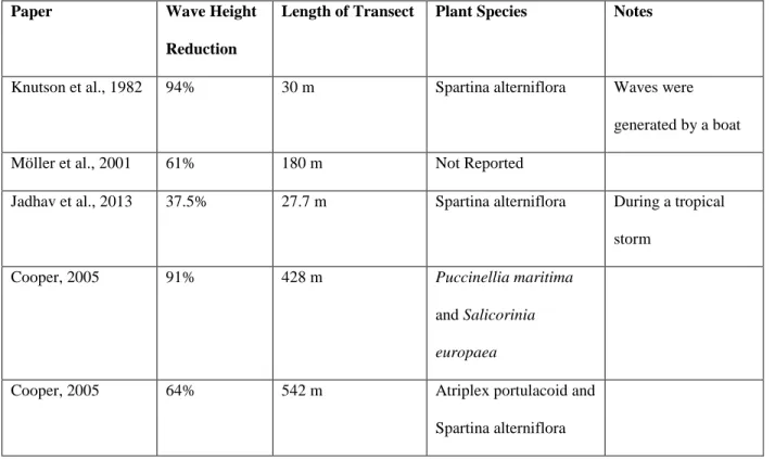
table below shows data from several different studies and demonstrates how wide the observed
rates of wave attenuation have ranged in various studies.
Table 1. Previous Studies Wave Attenuation Rates. The table below shows the rates of wave
attenuation found in previous, and the plant species in the marshes of each of those studies.
Paper Wave Height
Reduction
Length of Transect Plant Species Notes
Knutson et al., 1982 94% 30 m Spartina alterniflora Waves were
generated by a boat
Möller et al., 2001 61% 180 m Not Reported
Jadhav et al., 2013 37.5% 27.7 m Spartina alterniflora During a tropical
storm
Cooper, 2005 91% 428 m Puccinellia maritima
and Salicorinia
europaea
Cooper, 2005 64% 542 m Atriplex portulacoid and
4
Cooper, 2005 78% 387 m Atriplex portulacoid and
Salicorinia europaea
Yang et al., 2012 38% 15.5 m Spartina alterniflora
Möller et al., 2014 13.8-19.5%
Depending on
wave period
and height
40 m Elymus athericus,
Puccinellia maritima,
and Atriplex prostrata
Experiment done in a
large wave tank with
simulated storm
surge conditions
Differences in wave attenuation among previous studies are due to several factors.
Differences in the vegetation characteristics at different sites can affect the rates of wave
attenuation. An increase in vegetation density can cause an increase in wave attenuation
(Anderson and Smith, 2014). Additionally, taller vegetation can also increase the rate of wave
attenuation. This is due to the fact taller vegetation reaches the upper part of the water column a,
where the orbital velocity is the greatest and therefore it can cause drag there (Tempest et al.,
2015). Spartina alterniflora is a common marsh species in North Carolina where this study was
conducted and previous studies have found that when compared to shorter plant species, Spartina
alterniflora results in greater wave attenuation (Tempest et al., 2015).
Differences in marsh topography can also affect wave attenuation rates. Obstacles such as
oyster reefs can act as breakwaters and reduce wave energy (Scyphers et al., 2011). Additionally,
wave height can increase due to shoaling, where waves increase in height when they reach
shallower water, often before eventually breaking and losing energy. This wave breaking
contributes to the overall loss in energy of the waves (Mendez and Losada, 2004).
Finally wave and water conditions can also affect wave attenuation rates. Waves with
5
motion of the vegetation. A study 2009 study found that seagrass moved in phase with the lower
frequency waves, but out of frequency with the higher frequency waves causing them to be
attenuated more (Bradley and Houser, 2009). The same mechanism could occur in saltmarshes,
although the grasses typically found in coastal North Carolina marshes, Spartina alterniflora and
Juncus roemerianus. Additionally, the Keulegan Carpenter number, which is the ratio of wave
orbital excursion to plant diameter, increases with increasing wave period, and the larger the
Keulegan Carpenter number, the smaller the drag coefficient of the vegetation (Mendez and
Losada, 2004). Water depth can also affect attenuation rates in that less attenuation occurs in
deeper water. Plant height affects how influential water depth is on the rate of wave attenuation.
A case study with marshes in Yangtze estuary in China found that the ratio of water depth to
plant height was inversely correlated with the attenuation rate (Yang et al., 2012). At greater
water depths, more vegetation is submerged and therefore, it has little effect on the upper part of
the water column where the orbital velocity is greatest (Augustin et al., 2009).
This study examines several of the factors that influence wave attenuation rates:
vegetation height, vegetation density, marsh bottom topography, water depth, and wave period.
We did this by examining wave heights at four different sites where these characteristics
differed, whereas many previous wave attenuation studies only examine one or two sites.
Additionally, this study compares wave attenuation data from one marsh site during storm and
everyday (normal) conditions.
2.
Methods
A. Data Collection
Four salt marsh sites were chosen to study wave attenuation, Crab Point, Deerfield, Pine
6
Carolina. Bogue Watch is on the North side of Bogue Sound and Pine Knoll Shores is on the
South side. Crab Point is on the Southwest side of the Newport River Estuary and Deerfield is
on the Northeast side. The GPS coordinates of each of the sites are in Table 2. The vegetation
communities of these marshes are dominated by Spartina alterniflora, with some Juncus
roemerianus present at Pine Knoll Shores.
Figure 1. Locations the four study Sites in Carteret County, North Carolina. Study sites are
7
Table 2.Site and Deployment Characteristics.
Deployment Coordinates Dates Recorded Vegetation Type Vegetation Height (cm) Vegetation Density
(m-1)
Crab Point- 1st Deployment 34.75179°N 76.70914°W 08/29/2016- 09/1/2016 Spartina alterniflora Mean: 55.1
Std. Dev.: 43.8
Mean: 0.72
Std. Dev.: 0.52
Deerfield 34.76158°N 76.66827°W 09/16/2016- 09/19/2016 Spartina alterniflora Mean: 55.4
Std. Dev.: 38.1
Mean: 1.63
Std. Dev.: 1.99
Bogue Watch 34.70691°N 76.96760°W 10/17/2016- 10/20/2016 Spartina alterniflora Mean: 20.6
Std. Dev.: 11.1
Mean: 1.95
Std. Dev.: 0.69
Pine Knoll Shores 34.69596°N 76.84181°W 11/11/2016-11/14/2016 Spartina alterniflora and Juncus roemerianus Mean: 44.2
Std. Dev.: 29.4
Mean: 1.30
Std. Dev.: 1.19
Crab Point-2nd Deployment (storm) 34.75179°N 76.70914°W 10/07/2016-10/10/2016 Spartina alterniflora Mean: 55.1
Std. Dev.: 43.8
Mean: 0.72
8
Figure 2. Sensor Locations in the Salt Marsh.The sensors are indicated by blue circles. The front
of the marsh is labeled at the bottom and is where the marsh meets the body of water, either the
Newport River or Bogue Sound.
At each site, five pressure sensors (RBR XR-620D) were placed in the ground at zero,
five, ten, twenty, and thirty meters from the marsh edge, along a line perpendicular to the
shoreline (Figure 2). The instruments were mounted pressure sensor upward so that the top of the
sensor and pressure measurement was 5 to 10 cm above the surface of the marsh. The sensors
were left at the marsh sites for six days, where they measured pressure at a rate of 6 Hz. Of the 5
sensors, four recorded data for 6 days and 1 sensor recorded for only 3 days. The sensors were
deployed twice at Crab Point, once during normal conditions and a second time during the
passage of a category 1 hurricane, Hurricane Matthew. Hurricane Matthew passed, at its closest,
approximately 70 miles East of the sites on October 9th, 2016 when it’s sustained winds were at 70 knots (130 km/hr) (Stewart, 2017). The maximum sustained wind speed observed in the
vicinity of the sites, at the NOAA NDBC Beaufort station (BFTN7), was 20 m/s (70 km/hr) from
the North. The sensors were deployed once at all other sites. The dates of the data recorded for
each deployment are in Table 2.
The elevation of the marshes was measured in a 5-m by 5-m grid using a laser level
(Topcon RL-H3C) and stadia rod, which allowed measure of the elevation of the marsh surface
shore-9
perpendicular transect of each marsh where the sensors were placed.
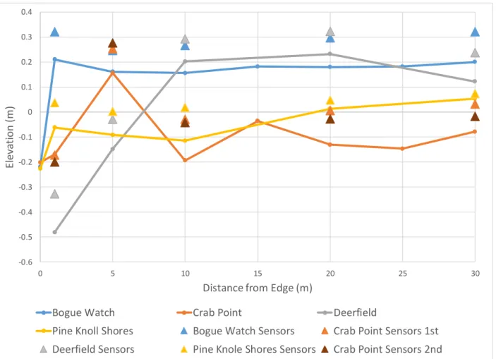
Figure 3. Marsh surface elevation, relative to NADV 88, of the shore-perpendicular transect
along which pressure sensors were placed. 0 m corresponds to the seaward edge of the marsh.
The elevations of the sensors are marked with triangles.
Bogue Watch rises steeply in the first meter then flattens out. The first sensor was placed
on the initial flat part of the marsh, at 1 m. Crab Point has an oyster berm at 5 m and then has
relatively little change in elevation thereafter. Deerfield has a steep slope within the first 10
meters, but then remains basically flat. Pine Knoll Shores has a small rise in the first meter, and
then gradually rises in elevation.
-0.6 -0.5 -0.4 -0.3 -0.2 -0.1 0 0.1 0.2 0.3 0.4
0 5 10 15 20 25 30
El ev at io n ( m )
Distance from Edge (m)
Bogue Watch Crab Point Deerfield
10
Spatially specific data on marsh vegetation species and the shoot height, diameter, and
density of each species were obtained from the NOAA Ecological Effects of Sea Level Rise
project (Voss, C., unpublished data). The vegetation was sampled in three haphazardly placed
25-cm by 25-cm quadrats placed at 1 m, 5 m, 10 m, 20 m, and 30 m from the edge of the marsh,
around the area wave attenuation was measured. See Table 2 for the mean plant heights and
densities.
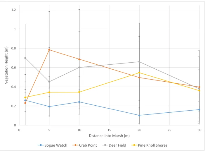
Figure 4. Vegetation height throughout the marsh from 1 m from the seaward marsh edge to 30
m. Values plotted are the mean height from three 25 cm x 25 cm sampling quadrats. The error
0 0.2 0.4 0.6 0.8 1 1.2
0 5 10 15 20 25 30
V e ge ta ti o n H e ig h t (m )
Distance into Marsh (m)
11
bars are the standard deviation of the vegetation heights across the three quadrats at each
distance in the marsh.
Bogue Watch consistently has the shortest vegetation. Crab Point has very short
vegetation near the marsh edge, followed by the tallest average vegetation in any of the marshes
at 5 m. The vegetation then gets shorter from 5 m to 30 m from the marsh edge. There was a
large variability in vegetation height within each site. The differences in heights at each site was
larger than the differences between sites. Deerfield has tall vegetation overall and has vegetation
heights most similar to those at Crab Point. Pine Knoll Shores has shorter vegetation in
comparison, though it is still taller than Bogue Watch.
0 1 2 3 4 5 6 7 8 9
0 5 10 15 20 25 30 35
D e n si ty ( m -1)
Distance from Marsh Edge (m)
12
Figure 5.Vegetation Density in each marsh from 1 to 30 m from the marsh edge. Vegetation
density is number of plants in each quadrat multiplied by the mean diameter of plants in that
quadrat divided by the area in the quadrat (625 cm2). Densities plotted are the mean values for three quadrats at each distance from the marsh edge and error bars indicate standard deviations.
Bogue Watch has a high vegetation density throughout the marsh, though at 5 m from the
marsh edge there is a notable decrease in density, compared to the rest of the site. Crab Point has
low vegetation density throughout the marsh. Deerfield has a large peak in vegetation density at
10 m from the marsh edge. Pine Knoll Shores has a smaller peak in vegetation density at 20 from
13
Figure 6.Vegetation frontal surface area in each marsh from 1 to 30 m from the marsh edge.
Vegetation frontal surface area is number of plants in each quadrat multiplied by the mean
diameter of plants multiplied by the mean height of the plants in that quadrat divided by the area
in the quadrat (25 cm2). Surface areas plotted are the mean values for three quadrats at each distance from the marsh edge and error bars indicate standard deviations.
Bogue Watch has low vegetation frontal surface area throughout the marsh. Crab Point
has low vegetation frontal surface area at 1, 20, and 30 m from the edge of the marsh, but a
larger vegetation density at 5 and 10 m. Deerfield has a large peak in vegetation frontal surface
0 0.5 1 1.5 2 2.5 3 3.5 4
0 5 10 15 20 25 30
Veget at io n S u rf ac e A rea p er S q u ar e M et er
Distance from Edge (m)
14
area at 10 m from the marsh edge. Pine Knoll Shores has a smaller peak in vegetation frontal at
20 m from the marsh edge.
B. Analysis
In order to isolate the pressure that was caused by the water above each sensor,
atmospheric pressure was subtracted from the total pressure measured by the sensor.
Atmospheric pressure came from NOAA’s National Data Buoy Center, from the Cape Lookout
station. The pressure record was divided into 5-minute intervals and the mean pressure was
calculated for each interval. Then, using the density of water (1000 kg/m3), the water depth above each sensor was calculated from the mean pressure. I then created a pressure spectrum,
which is the variance of pressure per unit frequency versus frequency. This spectrum was then
converted to a surface elevation spectrum, using the relationship between wave height and
pressure from linear wave theory (Dean and Dalrymple, 1984):
2 2 cosh ) ( cosh ) ( kz z h k g p S
(1)
Where S is the surface elevation spectrum, p is pressure, ρ is density, g is acceleration
due to gravity, k is wavenumber, z is distance above the marsh bottom, t is time, H is wave
height, and h is water depth. At high frequencies the noise in the data overwhelms the actual
data, causing an overestimation of the surface elevation variance actually occurring at those
frequencies. The spectrum was therefore cut off above a threshold frequency. The cutoff
15
floor. A f-4 decay was placed on the end of each spectrum beyond the cutoff frequency to
estimate the waves at the high frequencies (Jones and Monismith, 2007).
The integral of the surface elevation spectrum was then computed to get the total variance
of the surface level fluctuations. We then took the square root of this variance to get the standard
deviation, and then multiplied that by four to get the significant wave height. The mean incident
significant wave heights for each deployment are in Table 3.
In order to calculate the mean period (Tm), the following equation was used:
1 0 0 ( ) ( ) nf m nf
f F f df T
F f df
(2)
Where f is frequency and F(f) is the water surface elevation spectrum, and nf is the smallest
frequency of wave able to be measured. See Table 2 for the mean of the mean periods of the
incident waves observed during each deployment.
3.
Results
A. Conditions during deployments
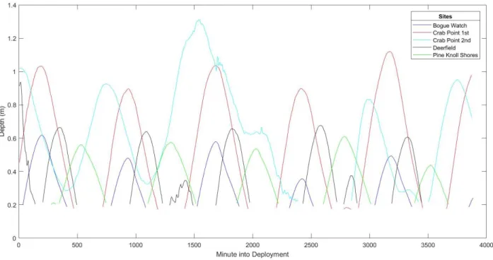
There were a variety of water depth ranges during each of the deployments (Figure 6), with
maximum depths over the marsh platform ranging from 0.6 m to over 1.2 m. The second
16
depths reaching above 1.2 m at one point. The first deployment at Crab Point had the next
deepest depths, with maximum depths above 1 m. The deployments at Deerfield, Bogue Watch,
and Pine Knoll Shores had much shallower depths by comparison.
Figure 7. Water depths at the 10-m sensor in a time series throughout the deployments. The gaps
in the time series represent times where there was not at least 10 cm of water above the sensor.
Incident significant wave height also varied significantly between deployments at
different sites (Figure 7). The deployment with the largest waves was the second Crab Point
deployment, which was during storm conditions. Deerfield had the smallest waves, with most of
the waves never going above 0.10 m. During all the deployments during regular conditions,
waves remained mostly small, with most of the wave heights less than 0.20 m. Table 3
17
Figure 8.Incident Significant Wave Height Histograms during each deployment. On the x axis is
the significant wave height and on the y axis is the number of 5-min intervals that had this
significant wave height. Each separate plot represents a separate deployment.
Table 3. Wave Conditions During Deployments.
Sites Significant Wave Height (cm) Mean Period (s)
Crab Point- 1st Deployment Mean: 14.11
Std. Dev: 4.87
Mean: 1.19
Std. Dev: 0.21
Deerfield Mean: 3.44
Std. Dev: 2.31
Mean: 1.56
Std. Dev: 0.51
Bogue Watch Mean: 7.78
Std. Dev: 3.04
Mean: 0.98
Std. Dev: 0.19
Pine Knoll Shores Mean: 10.04
Std. Dev: 4.49
Mean: 1.47
Std. Dev: 0.28
Crab Point-2nd Deployment
(storm)
Mean: 18.60
Std. Dev: 7.73
Mean: 1.73
18
The second deployment at Crab Point, during storm conditions, had the largest waves and the
waves with the longest periods. During regular conditions, Crab Point had the largest waves,
followed in decreasing order by Pine Knoll Shores, Bogue Watch, and Deerfield. Deerfield had
the waves with the longest periods during regular conditions, followed in decreasing order by
Pine Knoll Shores, Crab Point, and Bogue Watch.
B. Wave Attenuation
The reduction of height of the waves was calculated by dividing the significant wave height
at each sensor by the incident significant wave height. I split the reductions in wave height into
categories based on different water depths during the deployments (Figures 9-12).
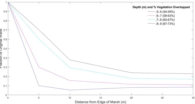
Deerfield shows little attenuation in the first ten meters, followed by a steep drop off in
wave height beyond this distance from the marsh edge (Figure 9). This could be due to the
vegetation density and the topography at Deerfield. The density of the vegetation is low at
Deerfield at 0 and 5 m, but is very high at 10 m (Figure 5). A greater density in vegetation would
provide greater resistance to the propagation of wave energy in the marsh by causing an increase
in friction. Additionally, the topography at Deerfield rises from the edge of the marsh to 10 m
from the marsh edge (Figure 3). This could cause shoaling, which would cause an initial increase
in wave height. Therefore, in the first 10 m from the marsh edge there would be both a decrease
in wave height at Deerfield due attenuation and an increase in wave height due to shoaling.
At Crab Point, wave attenuation was also likely influenced by topography. During the
19
10). This is may be due to the oyster berm that occurs at 5 m from the marsh edge at the site
(Figure 3). The oyster berm would cause a loss of energy from the waves due to bottom friction
and possibly wave breaking, thus reducing their height.
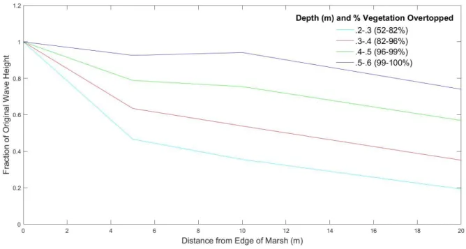
Pine Knoll Shores (Figure 12) and Bogue Watch (Figure 11) have less wave attenuation
than the first deployment at Crab Point (Figure 10) and Deerfield (Figure 9), especially at higher
water depths. This may be due to the fact that the vegetation at Pine Knoll Shores and Bogue
Watch is shorter than the vegetation at Crab Point and Deerfield (Figure 4). Taller vegetation
would affect the wave motion throughout more of the water column, so it reduces wave height
more than shorter vegetation.
All deployments show the general trend of less wave attenuation at deeper depths.
However, this trend differs in its strength between different deployments. The trends in wave
height attenuation with increasing water depth are summarized in Figure 13 and Table 4. The
first deployment at Crab Point (Figure 11) and Deerfield (Figure 9) do not have as dramatic a
difference in attenuation rate between different water depths as Pine Knoll Shores (Figure 12)
and Bogue Watch (Figure 11). Again, this may be due to the fact the vegetation at Crab Point
and Deerfield is taller than vegetation at Pine Knoll Shores and Bogue Watch. Figure 14 supports
this hypothesis and shows how the taller the vegetation, the greater the rate of decline of wave
attenuation with increasing depth.
The first and second deployments at Crab Point have very different patterns of wave
attenuation. The second deployment (Figure 13), which was during storm conditions, does not
show as much wave attenuation as the first deployment (Figure 10). Additionally, there is greater
separation of rates of attenuation between water depths during the second deployment. Water
20
difference between the two deployments, since during similar water depths wave attenuation
rates were smaller during the second deployment.
Figure 9.Wave height reductions (y-axis) at different distances from the marsh edge (x-axis) at
Deerfield. Each colored line represents a different water depth range. The numbers in
parentheses in the legend show the percentage of vegetation overtopped (completely submerged)
21
Figure 10. Wave height reductions (y-axis) at different distances from the marsh edge (x-axis) at
Crab Point during the first deployment (normal conditions). Each colored line represents a
different water depth range. The numbers in parentheses in the legend show the percentage of
22
Figure 11. Wave height reductions (y-axis) at different distances from the marsh edge (x-axis) at
Bogue Watch. Each colored line represents a different water depth range. The numbers in
parentheses in the legend show the percentage of vegetation overtopped (completely submerged)
23
Figure 12. Wave height reductions (y-axis) at different distances from the marsh edge (x-axis) at
Pine Knoll Shores. Each colored line represents a different water depth range. The numbers in
parentheses in the legend show the percentage of vegetation overtopped (completely submerged)
24
Figure 13. Wave height reductions (y-axis) at different distances from the marsh edge (x-axis) at
Crab Point during the second deployment, which included the passage of Hurricane Matthew.
Each colored line represents a different water depth range. The numbers in parentheses in the
legend show the percentage of vegetation overtopped (completely submerged) at those water
25
Figure 14.Reduction of wave height at 20 m into the marsh versus water depth for all
deployments. The color of the dots indicates different deployments. The lines are lines of best fit
for each of the deployments and are also colored to indicate the deployment.
Table 4.Equations and r-squared values of lines of best fit for the relationship between wave
height decline and water depth in Figure 13. For equations in the middle column, y is the
percentage of wave height decline by 20 m from the marsh edge and x is the depth of the water
on the marsh platform, according to the 10-m sensor.
Deployment Line of Best Fit R-squared value
Bogue Watch y=-137.9x+112.3 0.96
Deerfield y=-23.5x+74.8 0.72
Pine Knoll Shores y=-72.1x+62.5 0.99
26
Figure 15.Slopes of relationships between water depth and wave height reduction from Figure
13, plotted against mean vegetation height.
C. Wave Period
Figures 16-20 display histograms of mean wave periods during each of the deployments at
different distances from the marsh edge. There was a general trend of waves with longer periods
27
to the left, towards the longer periods. This trend is most prominent during the deployment at
Pine Knoll Shores (Figure 18) and during the first deployment at Crab Point (Figure 19). The
trend is present at Bogue Watch. It is much less prominent at Deerfield (Figure 17) and during
the second deployment at Crab Point (Figure 20).
There are differences in the periods of incident waves between sites. The incident waves at
Deerfield (Figure 17) and at Crab Point (Figure 20) during the second deployment have a much
greater range of periods than during the other deployments. This difference of wave period range
may be why there is a difference in the attenuation rates between the first and second deployment
at Crab Point (Figures 11 and 12). Since there are more long period waves during the second
deployment at Crab Point, and waves with longer periods are attenuated less, this could explain
28
Figure 16. Histograms of the wave periods at different distances into the marsh at Bogue Watch.
The wave periods are on the x axis and the numbers of 5-minute intervals with a mean wave
29
Figure 17.Histograms of the wave periods at different distances into the marsh at Deerfield. The
wave periods are on the x axis and the number of waves are on the y axis. Each histogram shows
the wave periods at a different distance from the marsh edge, as indicated in the upper right
30
Figure 18.Histograms of the wave periods at different distances into the marsh at Pine Knoll
Shores. The wave periods are on the x axis and the number of waves are on the y axis. Each
histogram shows the wave periods at a different distance from the marsh edge, as indicated in the
31
Figure 19. Histograms of the wave periods at different distances into the marsh at Crab Point
during the first deployment. The wave periods are on the x axis and the number of waves are on
the y axis. Each histogram shows the wave periods at a different distance from the marsh edge,
32
Figure 20. Histograms of the wave periods at different distances into the marsh at Crap Point
during the second deployment. The wave periods are on the x axis and the number of waves are
on the y axis. Each histogram shows the wave periods at a different distance from the marsh
edge, as indicated in the upper right corner of each graph.
4.
Discussion
This study examined five factors that affect wave attenuation rates in salt marshes: water
depth, vegetation density, vegetation height, marsh topography, and wave period. Overall, the
33
all deployments. Marshes with taller vegetation had more wave attenuation and the wave
attenuation varied less with water depth, when compared to marshes with shorter vegetation.
This trend is most likely due to the tall vegetation’s ability to occupy the top portion of the water
column where the orbital velocity is greatest for a larger range of water depths. It has been
previously observed that emergent vegetation is more effective at damping waves than fully
submerged vegetation (Augustin et al., 2009). If the vegetation in a marsh is short, then it is more
likely to be fully submerged, and less effective at damping waves, at shallower water depths.
Additionally, if vegetation is short, then the fraction of the water column occupied by vegetation
will vary more as water depth varies than if vegetation is tall.
Greater vegetation density and surface area was also associated with higher rates of wave
attenuation. This is most likely due to the greater surface area opposing the wave energy, a
combination of greater stem diameter, more plants, and or taller plants. All three of these factors
varied from site to site and within sites. At one of the sites, Deerfield, there was a steep drop in
wave height after a particularly dense area of vegetation.
Additionally, the steep upward slope of one of the marsh bottoms at Deerfield may have
induced wave shoaling. Shoaling initially increases wave height, but when the waves break
energy is dissipated. This could be another one of the reasons why wave height did not
significantly decrease initially at this site, but then decreased rapidly after the marsh bottom
stopped sloping upwards and became flatter. Another marsh bottom feature may have induced
energy dissipation Crab Point. There was an oyster berm there which could have acted as a
breakwater and dissipated the wave energy. Crab Point had a large drop in wave height around
the oyster berm, and the magnitude of this drop in wave height was a strong function of water
34
Wave period also appeared to have an effect on wave attenuation. Waves of higher
frequencies (shorter periods) were typically attenuated more than waves of lower frequencies
(longer periods). This trend was stronger at some sites than others. This period-dependent
attenuation rate has been observed in another study examining wave attenuation in seagrass
where it was attributed to the motion of the grass (Bradley and Houser, 2009). Seagrass moved in
phase with the lower frequency waves, but out of phase with the higher frequency waves,
effectively acting as a filter for the higher frequency waves. Grass motion could also affect
attenuation in marsh grass causing similar effects. Frequency dependent attenuation may also
have to do with Keulegan Carpenter number. The Keulegan Carpenter increases with increasing
period, and in models of wave damping, a bigger Keulegan Carpenter means a reduced drag
coefficient and thus less resistance acting on the wave motion (Mendez and Losada, 2004).
There was also a large difference between the patterns of wave attenuation observed
during a storm and those observed during everyday conditions. Attenuation during the storm was
smaller overall than normal conditions, despite water depths being similar. The incident wave
periods were longer during the storm conditions and, as previously explained, waves with longer
periods are attenuated less than waves with shorter periods.
Within this study it is difficult to separate out the causes of wave attenuation to determine
which has the largest effect on the variance between the rates during the different deployments.
In order to do this, one would need to develop a process based model, such as the model
developed explained in Mendez and Losada, 2004.
The attenuation rates during normal conditions in this study are most similar to those
found in Knutson et al. 1984 and Yang et al., 2012. During the second deployment at Crab Point,
35
Overall, the rates observed in this study are within the range of attenuation rates found by other
studies in Spartina alterniflora marshes.
5.
Conclusion
This study examined various factors affecting wave attenuation in salt marshes. Taller
and denser vegetation was associated with higher rates of wave attenuation. Marsh topography
played a role in reducing wave energy. A raised area near the front of the marsh acted as a
breakwater, which dissipate and refract wave energy, and a steep slope at the front edge of
another marsh was thought to cause wave shoaling. Finally, waves with longer periods were
attenuated less than waves with shorter periods, though the strength of this trend varied from site
to site. Under storm conditions, waves periods were longer, which may be what caused smaller
rates of wave attenuation during storm conditions than during regular conditions.
These findings have implications for using salt marshes in living shorelines to attenuate
wave energy. When constructing marshes, tall and dense vegetation should be used and one
might consider installing features like oyster berms to act as a breakwater. Also, marshes are
more likely to be effective at protecting shorelines in areas with short fetches, where wave
periods are shorter.
More study is needed on why wave attenuation varies more strongly with wave period on
some marshes than others. Additionally, future studies should look at the differences in wave
attenuation at Spartina alterniflora dominated versus Juncus roemerianus dominated marshes.
Those plants have different morphologies, with Spartina being a cord grass with leaves and
Juncus being needle like, and may have different attenuation abilities. Both species are common
36
In conclusion, salt marshes are capable of attenuating waves to protect shorelines, though
the rates of attenuation vary with vegetation, morphological, wave period, and depth.
6.
References
Anderson, ME, and JM Smith. "Wave Attenuation by Flexible, Idealized Salt Marsh Vegetation."
Coastal Engineering, vol. 83, 2014, pp. 82-92.
Augustin, L. N., J. L. Irish, and P. Lynett. 2009. "Laboratory and Numerical Studies of Wave Damping
by Emergent and Near-Emergent Wetland Vegetation." Coastal Engineering, vol. 56, no. 3,
2009, pp. 332-340.
Barbier, E. B., Hacker, S. D., Kennedy, C., Koch, E. W., Stier, A. C., and Silliman, B. R. (2011). The
value of estuarine and coastal ecosystem services. Ecological Monographs, 81(2),
2011,pp.169-193.
Bradley, K., and Houser, C. "Relative Velocity of Seagrass Blades: Implications for Wave Attenuation
in Low-Energy Environments." Journal of Geophysical Research - Earth Surface, vol. 114, no.
F1, 2009, pp. F01004.
Cooper, N. J. "Wave Dissipation Across Intertidal Surfaces in the Wash Tidal Inlet, Eastern England."
Journal of Coastal Research, vol. 21, no. 1, 2005, pp. 28-40.
Costanza, R., Pérez-Maqueo, O., Martinez, M. L., Sutton, P., Anderson, S. J., & Mulder, K. "The
Value of Coastal Wetlands for Hurricane Protection." Ambio: A Journal of the Human
Environment, vol. 37, no. 4, 2008, pp. 241-248.
Dean, Robert and Robert Dalrymple. Water Wave Mechanics for Engineers and Scientists.
37
Jadhav, R. S., Chen, Q., and Smith, J. M. "Spectral Distribution of Wave Energy Dissipation by Salt
Marsh Vegetation." Coastal Engineering, vol. 77, 2013, pp. 99-107.
Jones, N. L., and S. G. Monismith. Measuring short-period wind waves in a tidally forced environment
with a subsurface pressure gauge. Limnol. Oceanogr. Methods, 2007.5: 317-327.
Knutson, P. L., R. A. Brochu, W. N. Seelig, and M. Inskeep. "Wave Damping in Spartina Alterniflora
Marshes." Wetlands 2.1, 1982, pp. 87-104.
Mendez, FJ, and IJ Losada. "An Empirical Model to Estimate the Propagation of Random Breaking
and Nonbreaking Waves Over Vegetation Fields." Coastal Engineering, vol. 51, no. 2, 2004, pp.
103-118.
Möller, I., Spencer, T., French, J. R., Leggett, D. J., and Dixon., M. "The Sea-Defence Value of Salt
Marshes: Field Evidence from North Norfolk." Water and Environment Journal 15.2, 2001, pp.
109-16. Wiley Online Library. Web. 4 Oct. 2016.
Moller, I., et al. "Wave Attenuation Over Coastal Salt Marshes Under Storm Surge Conditions."
Nature Geoscience, vol. 7, no. 10, 2014, pp. 727-731.
Scyphers, S. B., Powers, S. P., Heck Jr, K. L., & Byron, D. "Oyster Reefs as Natural Breakwaters
Mitigate Shoreline Loss and Facilitate Fisheries." Plos One, vol. 6, no. 8, 2011, pp. e22396.
Shepard, C. C., Crain, C. M., and Beck, M. W. "The Protective Role of Coastal Marshes: A Systematic
Review and Meta-Analysis." Plos One, vol. 6, no. 11, 2011, pp. e27374.
Tempest, J. A., Möller, I. and Spencer, T. "A Review of Plant-Flow Interactions on Salt Marshes: The
Importance of Vegetation Structure and Plant Mechanical Characteristics: Salt Marsh Plant-Flow
38
Yang, S. L.,Yang, S. L., Shi, B. W., Bouma, T. J., Ysebaert, T., & Luo, X. X. "Wave Attenuation at a
Salt Marsh Margin: A Case Study of an Exposed Coast on the Yangtze Estuary." Estuaries and