COMPARING THE OPTIMAL ALLOCATION IN STRATIFIED AND POST-STRATIFIED SAMPLING USING MULTI-ITEMS

COMPARING THE OPTIMAL ALLOCATION IN

STRATIFIED AND POST-STRATIFIED SAMPLING

USING MULTI-ITEMS

F. S. APANTAKU

Department of Statistics, Federal University of Agriculture, Abeokuta, Nigeria *Corresponding author: [email protected] Tel: +2348037183877

commonly used in all fields of scientific in-vestigation is that of probabilistic sampling. Probability sample designs can be made bet-ter with features to assure representation of population subgroups in the samples and stratification is one of such features. Surveys used by social scientists are based on com-plex sampling designs (Lumley, 2004; Win-ship and Radbill, 1994).

ABSTRACT

Usually in sample surveys more than one population characteristics are estimated (multi-item). These characteristics may be of conflicting nature. Optimal allocation using a stratified random sample solves the statistical problem that may be found with proportional allocation, by ensuring that enough re-spondents are studied in each segment to provide the highest level of accuracy for the overall results. The study compared optimum allocation in stratified and post stratified sampling using multi-items and determined the variations of the components of the multi-items in the proposed model. The idea of optimum allocation based on the multi-items was approached using a linear programming problem that minimizes the covariance of the stratified variable subject to a fixed cost. The covariance matrix was defined based on the four socio-economic characteristics of 400 heads of household in Abeokuta South and Ijebu North Local Government Areas of Ogun State, Nigeria. The characteristics were occu-pation, income, household size and educational level. The data from the survey was transformed for each of the four characteristics. The estimates used in the computation were calculated using statisti-cal analysis software Splus. From the analysis, it was seen that for both Abeokuta and Ijebu data sets, the variance based on the four characteristics as multivariate is less than that of the variables when considered as a univariate. From the results, it was seen that there was no difference in the percent-age of the total variance accounted for by the different components from the merged sample when compared with the individual sample.

Key words: Optimum allocation, stratified sampling, post stratified sampling, multi-items, optimization

INTRODUCTION

In social research, special emphasis is placed on the comparative and analytical use of samples. Knowledge, attitudes, and actions in life everyday are based to a very large extent on samples (Cheang, 2011; Cochran, 1977). In survey, samples are used instead of population and most of the-se samples are prepared by Statisticians and one of the areas of Statistics that is most

Journal of Natural Science, Engineering

and Technology ISSN:

Print - 2277 - 0593 Online - 2315 - 7461 © FUNAAB 2014

One of the main problems in sampling sur-vey is the optimal allocation of resources. Usually, the solution of such problem is rather arbitrary due to the fact that no best allocation is defined. In terms of this model, the allocation problem is to find the alloca-tion of a sample to strata which minimizes cost of investigation subject to a given con-dition about the sampling error.

An effective sampling technique within a population represents an appropriate ex-traction of useful data which provides meaningful knowledge of the important aspects of the population (Diaz-Garcia and Cortez, 2006). Probability sampling meth-ods are usually designed to be measurable, that is, so designed that statistical inference to population values can be based on measures of variability, usually standard er-rors, computed from the sample data. Empirical research may be performed in different ways: by haphazard observations, controlled observations, experiments, or surveys. This study concentrates on sam-pling for surveys. Survey research is aimed at estimating specified population values. A population value is a numerical expression that summarizes the values of some charac-teristic(s) for all elements of an entire popu-lation. It is a summary measure of some features of the distribution of the variable(s) in the defined population. The population is defined jointly with the elements. The pop-ulation is the aggregate of the elements, and the elements are the basic units that com-prise and define the population. The popu-lation must be defined in terms of content, units, extent and time (Cheang, 2011). The survey population achieved may differ somewhat from the desired target popula-tion. The major difference frequently arises

from non responses and non coverage and only the survey population is represented in the sample. The sample provides statistical inference to the survey population. Behind every survey population stands some hypo-thetical universe, explicit or implicit, definite or indefinite. Characteristics of population elements are transformed to variables by the survey operations of measurement and a sta-tistic based on the variables found in a sam-ple results in a random variable which is called a variate. Any population value is de-termined by four factors (a) the defined sur-vey population; (b) the nature of the sursur-vey variable (s) and their distributions in some cases; (c) the method of observations; and (d) the mathematical expression for deriving the population value from the individual ele-ment values (Kolenikov, 2010).

In random sampling, stratified random sam-pling can produce a more concentrated dis-tribution of estimates. This suggests that stratification can produce sample statistics which are more precise or which have small-er small-error due to sampling than simple random samples. Stratification in this study is to al-low the investigation of the characteristic of interest for particular subgroups by ensuring adequate representation from each subgroup of interest (Lumley, 2004; Sethna and Groeneveld, 1984).

Stratification by making use of existing knowledge concerning the population pro-vides an effective means of reducing the measured variability of estimates. The popu-lation variability itself does not change but the technique for calculating variability via stratification offers the possibility, when done successfully, of reducing the variance estimate of the population (Sethna and Groeneveld, 1984). Lower measured variabil-ity permits the researcher to make a more

precise estimate or it enables one to make an interval estimate at a lower cost. The stratification technique is also an effective means of assuring representation in the sample from each stratum in the popula-tion. Simple random sampling techniques offer no assurances that each segment of the population is represented. Stratification and subsequent sampling with strata assure this representation.

Post-stratification may be used on the sub-classes even if a proportionate sample of the entire population has been selected. Post stratification is an example of improv-ing the estimator by the proper utilization of ancillary sources of information. The method of using stratification is to increase the precision of the sample mean as in con-trast to proportionate sampling. It involves the deliberate use of widely different sam-pling rates for the various strata. Optimum stratification is used when the standard de-viations of the population strata are known to differ substantially. This technique is a method of allocating larger size samples to those strata with larger standard deviations. The designation optimum allocation to dis-proportionate sampling refers to the aim of assigning sampling rates to the strata in such a way as to achieve the least variance for the overall mean per unit of cost (Diaz-Garcia and Cortez, 2006).

Usually in sample surveys more than one population characteristics are estimated (multi-item). These characteristics may be of conflicting nature. Stratification may pro-duce a gain in precision in the estimates of characteristics of the whole population. It may possibly divide the heterogeneous pop-ulation into sub-poppop-ulations, each of which it internally homogeneous.

Optimal allocation using a stratified random

sampling solves the statistical problem that may be found with proportional allocation, by ensuring that enough respondents are se-lected and studied in each stratum to provide the highest level of precision for the overall results.

The objectives of the study are to:

a. Compare optimum allocation in stratified and post stratified sampling using multi-items, and

b. Determine the variations of the compo-nents of the multi-items in the model

improved tremendously on what I meant on ground, in terms of record keeping which are readily available for checking. proposed.

METHODOLOGY

The procedure for estimation from multiple frames was given by Hartley (1962, 1964). According to Hartley, choosing a simple cost function provides rules for optimal choices of subject to a given value. Saxens et al. (1986) considered the extension of Hartley’s procedure to the case of two stage sampling of the multi-stage sampling. They worked out optimal choices of the variable of inter-est considering suitable cost functions and recommended replacement of unknown pa-rameters occurring in the optimal solutions by sample analogues. Hence the problem of small domain statistics and a special method of estimation is needed for the parameters relating to small domains. Bankier (1996) discussed a few issues involved in small area or local area estimation. The problem is how to estimate the domain. These estimators make a minimal use of data that may be available. To improve upon the estimators, the database is broadened and strengths are borrowed from data available on similar do-mains and secondary external sources. Ac-cording to Bankier (1996), post-stratified

estimators of auxiliary data, is to be used. These post strata may stand for age, sex, or ethnic groups in usual practices.

The multivariate stratified sample design

The multivariate stratified sample design is used for multi-objective surveys in which there is difference among the importance of interest variables. All these method consider the computation of the stratum sample size, which can be computed by various proce-dures, but optimum allocation has been found to be a useful approach. Optimum allocation in multivariate stratified sampling can be seen as a multi-objective tion problem and multi-objective optimiza-tion problem is a particular case of a matrix optimization.

Khan and Ahsan (2003, 1967) proposed a method in which they formulated multi-objective surveys as a nonlinear ming problem and use a dynamic program-ming technique to find a solution. One problem with this approach is how to weigh the variances. There is no single solution for doing this, and it is not always easy to pre-dict what the consequences of a particular choice of weights are.

The multivariate optimum allocation

The problem of allocating sample to various strata may be viewed as minimizing the vari-ances of various characters subject to the conditions of the given budget and tolerance limits on certain variances. The problem turns out to be nonlinear programming problem with several linear objective func-tions and single convex constraint. Pizada and Maqbool (2003), solved the resulting linear programming problem through Che-byshev approximation. The criteria behind the Chebyshev approximation are to find a solution that minimizes the single worst. Suppose that characteristics are meas-ured on each unit of a population which is partitioned into strata. Let be the number of units drawn from the

stratum ( For the

character an unbiased estimate of the popu-lation mean, is which has the sam-pling variance.

 p

L ni,

th i

). ,..., 2 , 1

(i L jth

,

j

Y y_jst

(2.1)

where

and in usual notation.

Let be the cost of enumerating the characteristic in the stratum and let be the upper limit on total cost of the survey. Then

p j

X S W y

Var _{ij i}

L

i i

jst) 1,2,....,

( 2

1 2





_



2 1

2

) (

1 1

, _ij

N

h ijth i

ij i

i y y

N S N N W

i

 





_



,

, 1

1 _{2 2}

ij i ij i i

i a W S

N n

X   

ij

c _{jth ith}

(2.2) The multivariate allocation problem can be stated as

Minimize Subject to

(2.3) where is used for If (34) is considered separately for each character, by ignoring the constant term in the objective function, the problem for character becomes

Minimize Subject to

(2.4)

By introducing a new variable the problem (3.75) transforms to Minimize (a)

Subject to

(b) (2.5)

(c)

(d)

 

 



L

i p

j i ijn k

c 1 1

p j

N a X

a z

L

i i ij i

L

i ij

j , 1,2,....,

1 1

 



_

_

 

k X c

L

i p

j i ij



 

1 1

L i

X

N_i i 1, 1,2,...,

1

  

i

X

1

.

i

n

th

k







L

i i ik k

X a Z

1

k X

c _i

L

i p

j

ij 

 

1 1

. ,..., 2 , 1 ,

1 X_i N_i i L

,

k L

x _

k L

k x

Z  _

0 )

(

1

 

 _





L k

L

i i ik

k X

X a X

g

k X

c i

L

i p

j

ij 

 

1 1

. ,.... 2 , 1 ,

The constraints in (2.5b) are convex (Kokan and Khan, 1967) and the constraint (2.5c) and the bounds (2.5d) are linear. The prob-lem (2.5a)-(2.5d) is therefore a convex pro-gramming problem with linear objective and can be solved by using any method of

convex programming. The Chebyshev ap-proximation formulation of the multiple ob-jective allocation problems in (2.5) is the fol-lowing linear programming problem (LPP): Minimize 

Subject to

(2.6)

0 2

1 (0) 1

) 0

(  2   









L k

L

i _ik i ik L

i k i

ik

X X

X a X

a

k i

L

i p

j

ijX k l t

c 1,2,...,

1 1

 

 

 

p k 1,2,...,

0

k k

L z

X _  

L i

N

X_{i i} 1,2,...,

1  

The solutions have

been obtained by minimizing the individual objective functions subject to the linearized constraints by letting the minimum values of to be found as

at the corresponding minimal points

p 20 0

0

1 ,X ,....,Xp

X

k

Z Z_k0, k1,2,...,p

This gives the aspiration levels being used in Chebyshev approxima-tion.

Formally the problem of optimum allocation in stratified sampling can be presented as a multi-objective, nonlinear optimization as

. ,...., 2 , 1 ,

0

p k

X_k 

Subject to (2.7)

Where C is the total cost, is the fixed cost and and

    

 

    

  

) ( ˆ

: :

) ( ˆ min ) ( ˆ min

1

G st st

n st

y ar V

y ar V y

ar V

C c n

c  ₀ 

0

c c(c₁,...c_H)

) ,... ,

(n₁ n₂ n_H n

The solutions in (2.7) take real values and the sample sizes must be integers. There is the problem of estimating the vari-ance on the basis of the sample size in each

h

n

stratum and also the problem of over sam-pling, that is, when for at least some

h h N

n 

.

h

An alternative to (2.7), is given as

where G is number of characteristics

subject to (2.8)

    

 

    

  

) ( ˆ

: :

) ( ˆ min ) ( ˆ min

1

G st st

n st

y ar V

y ar V y

ar V

C c n

c  ₀ 

H h

N

n_{h h} , 1,2,...,

2  

 

h

n

Where denotes the set of natural num-bers. The methods for resolving a multi-objective optimization programme can be classified by considering the amount of in-formation possessed concerning the study population, with three different scenarios, namely complete, partial or zero infor-mation (Steuer, 1986; Miettinen, 1999; Diaz -Garcia and Ulloa, 2006). Diaz-Garcia and Ulloa (2006) consider problem (2.8) from the stand-point of the multi-objective opti-mization methods by using complete infor-mation such as value function and lexico-graphic, partial information method such as

constraint and also zero information such as the distances.

Optimum allocation via multi-objective optimization

The estimator of the population mean in multivariate stratified sampling for the



 

-th characteristic is defined as

(2.9)

Where is the sample mean

in stratum of the -th characteristic, and is the value obtained for the -th unit in stratum of the -th characteris-tic. The Var is defined using the

pop-ulation variances which

are usually unknown, and therefore these are substituted by the sample variances

j

j h H

h h j

st W y

y

_



 1







h

n

h j hi h j

h y

n y

1

1

h j

j hi

y _i

h j

) ( j

st

y

, ,..., 2 , 1 ,

2 _{h H}

defined as

(2.10)

And thus is substituted by the

estimated variance which is

giv-en by

(2.11)

Value function

Under the value function technique, pro-gramme (2.8) is expressed as

(2.12)

Where is a scalar function that sum-marizes the importance of each of the vari-ances of the G characteristics. Evidently for every problem the value function may take an infinite number of forms and this constitutes the difficulty for the evalua-tor in defining such a function. Some sim-ple functions have given excellent results in applications and one of these particular forms is the weighting method. Under the

, ,..., 2 , 1 ,

2 _{h H}

s_h 

2 1 2 ) ( 1 1 h n i hi h

h y y

n s h   



 ) ar( Vˆ y_stj

), ar( Vˆ y_stj





    H h hj h H h h hj h j st N s W n s W y 1 2 1 2 2 ) ar( Vˆ N n H h N n y ar V v h h h st     ,..., 2 , 1 2 subject to )) ( ˆ ( min n ) ( v ) ( v

weighting approach, (2.12) can be expressed as

(2.13)

Such that

where weighs the importance of each characteristic. In the context of multi-objective optimization, (2.13) is without doubt the method that has been mostly thor-oughly studied. Its popularity is due to the fact that the value function is unique. The value function method is utilized for recur-rent studies in which over time, the results obtained using (2.13) help in reaching a bet-ter inference for future experiments, in which the appropriate weighting can be ap-plied.

Lexicographic method

This method like value function requires complete information on the phenomenon in order to create an important ordered hier-archy of the variances evaluated. Unlike the value function method, it is not necessary to know what weight to allocate to each charac-teristic, but only the order of importance they represent in obtaining the sample. In this case, to optimize programme (2.8), the variances of the characteristics must be or-dered by the evaluator, beginning with the

N n H h N n C c n c y ar V h h h h H h h j st G j j n      





  ,..., 2 , 1 , 2 subject to ) ( ˆ min 0 1 1  ; ,..., 2 , 1 0 , 1 1 G j j G j

j    



   j 

one presenting the most important charac-teristics, and then by descending order of importance, thus obtaining

(2.14) ) ( ˆ .., ),... ( ˆ ), (

ˆ 1 2 iG

st i

st i

st Var y Var y

y ar V

where is a permutation with the

desired, descending order of the set of super indices 1,2,….,G. To reach the stages in the vector, it is necessary to resolve the follow-ing programme

G

i i₁,...,

By letting be the minimum of problem (2.16), for the third stage the problem is re-solved as

(2.17)

To reach stage G, the next problem to be resolved is as (2.18) 2 v N n H h N n C c n v N S W n S W v N S W n S y ar V h h h h H h h h H h h h h H h h h h h h i st n          











     ,..., 2 , 1 , 2 c W subject to ) ( ˆ min 0 H 1 h h 2 1 2 2 1 2 2 2 1 1 2 1 H 1 h 2 1 2 3 N n H h N n C c n v N S n S v N S W n S W v N S W n S y ar V h h h h G hG h hG H h h h H h h h h H h h h h h h i st n G           















          ,..., 2 , 1 , 2 c W -W : : W subject to ) ( ˆ min 0 H 1 h h 1 H 1 h 2 1 h H 1 h 2 1 2 h 2 1 2 2 1 2 2 2 1 1 2 1 H 1 h 2 1 2

Hence the vector obtained in this stage is the optimum solution to the problem. Optimal design for a multivariate stratified sampling adopted in the study

The idea of optimal allocation under a multivariate stratified sampling in the study is based on an alternative approach as in Diaz-Garcia and Ramos-Quiroga (2011).

The linear programming problem is assumed to be

Subject to

(2.19)

Where . This is the matrix of variance covariances of the vector

ỹst = (ỹst, ……….. ỹst).

the sub index h = 1,2, ….. H denotes the stratum i = 1,2,…..Nh or nh within stratum h and j = 1,2,…., G. denotes the characteristic (variable).

The covariance matrix of ỹ st denoted as cov (ỹst) is defined in matrix

Var (ỹ1_{st) Cov (ỹ}1_{st ỹ}2_{st) Cov(ỹ}1_{st ỹ}G_st) (2.20)

cov(ỹst) = Cov (ỹ2st, ỹ1st) Var (ỹ2st) Cov(ỹ2st ỹGst) Cov (ỹG_{st, ỹ}1_{st) Cov (ỹ}G_{st ỹ}2_{st) Var(ỹ}G_st)

and the estimated covariance of ỹi_{st and ỹ}j_{st as Cov (ỹ}i_{st and ỹ}j_{st). this Cov (ỹ}i_{st and ỹ}j_{st) Cov} (ỹi_{st and ỹ}j_{st) =}

Cov (ỹi_{st, ỹ}i_{st) = -}

(2.21)

and Cov (ỹi_{st, ỹ}i_{st) = -}

and Ch is the cost per G – dimensional sampling unit in stratum h and its vector C = ( C1, …………CG)1.



min

n





 

H

h h

hn C C

C

1

0

h h N

n 



2 ) (yst

Cov  

Principal component analysis

Optimal allocation in multi-item is devel-oped as a multivariate optimization problem by finding the principal components. This was done by determining the overall linear combinations that concentrates the variabil-ity into few variables. We then search for a set of mutually uncorrelated variables, each one being a linear combination of the original set of variables,

. One of the motivations for determining such a collection is in of, if we derive a set that concentrates the overall variability into the first few variables, it is perhaps easier to see what accounts for the variation in the data.

Indeed, if a few of the seem to ac-count for most of the variation in the data, then it could be argued that the effective dimensionality is less than P and this could result in a simplified analysis based on a smaller set of variables (Jolliffe, 2002; Khan and Ahsan, 2003; Garcia and Cortez, 2006). THE EMPIRICAL EXAMPLE (CASE) Data on four socioeconomic characteristics of 400 heads of households in Abeokuta South and Ijebu North Local Government

p

Y Y Y1, 2,...,

p

X X

X₁, ₂,...,

} {Y_i

Areas (LGAs) of Ogun State, Nigeria were investigated. This comprised of 200 house-holds from each LGA. The characteristics were occupation, income, household size and educational level.

RESULTS

The data from the survey was transformed for each of the four characteristics. Occupa-tion was transformed into: (1) unemployed (2) paid employment (3) self employment, while income into: (1) 0 – < N10,000; (2) N10,000 - < N20,000; (3) N20,000 and above. Household size was transformed into: (1) small (1-3); (2) moderate (4-7); (3) large (7 and above), while educational level was transformed into: (1) primary; (2) secondary; (3) tertiary. The estimates used in the com-putation were calculated using statistical analysis software Splus.

Stratification by making use of existing knowledge concerning the population pro-vided an effective means of reducing the measured variability of estimates. The popu-lation variability itself does not change but the technique for calculating variability via stratification offers the possibility. The strati-fication technique in this study divided up the population into sub-population or strata. The strata for the four characteristics are in Tables 3.1, 3.2, 3.3 and 3.4.

Table 3.1: Stratified Data on Occupation of Heads of Household in both Abeokuta South and Ijebu North

Strata Occupation Number in

Abeokuta South population

Number in Ijebu North population

1 Unemployed 10 2

2 Paid employment 47 54

3 Self employment 143 144

200 200

The merged stratified data for the four so-cioeconomic characteristics of Abeokuta

South and Ijebu North LGAs are shown in Table 3.5.

Table 3.2: Stratified Data on Income of Heads of Household in both Abeokuta South and Ijebu North

Strata Income N(000) Number in Abeokuta South population

Number in Ijebu North population

1 0 to under N10,000 42 28

2 N10,000< N20,000 73 91

3 N20,000 and over 85 81

200 200

Source: Field Survey, 2012

Table 3.3: Stratified Data on Dependant Size of Heads of Household in both Abeokuta South and Ijebu North

Strata Dependant Size Number in

Abeokuta South population

Number in Ijebu North population

1 Small (1 to 3) 138 140

2 Mrate (4 to 7) 58 55

3 Large (7 and over) 4 5

200 200

Source: Field Survey, 2012

Table 3.4: Stratified Data on Educational Level of Heads of Household in Abeokuta South and Ijebu North

Strata Educational Level Number in Abeokuta South population

Number in Ijebu North population

1 Primary 53 44

2 Secondary 74 85

3 Tertiary 73 71

200 200

Using the data set for Abeokuta and Ijebu, the general multi-objective optimisation pro-gramme as in (2.8) is

(2.22)

Subject to

Furthermore, we consider the following two programmes for the non linear minimizing of integers:

(2.23)

    

 

    

  

) ( ˆ

) ( ˆ min ) ( ˆ min

2 1

st st

n st

y ar V

y ar V y

ar V





 4

1

200

h h

n

3 , 2 , 1 , 2n_h N_h h

 

h

n

) (

ˆ 1

min

st

n

y ar V

Table 3.5: Stratified Data on Occupation, Income, Dependant Size and Educational Level of Heads of Households in Abeokuta South and Ijebu North

Item No.

Name Stratum

No. Name

Size of Stratum

Abeokuta South and Ijebu-North

1 Occupation 1 Unemployed

2 Paid employment 3 Self employment

12 101 287

2 Income (in

N’000)

1 0-10 2 10-20 3 20+

70 164 166 3 Dependant Size 1 Small (1-3)

2 Moderate (4-7) 3 Large (7+)

278 113 9

4 Educational

Level

1 Primary 2 Secondary 3 Tertiary

97 159 144

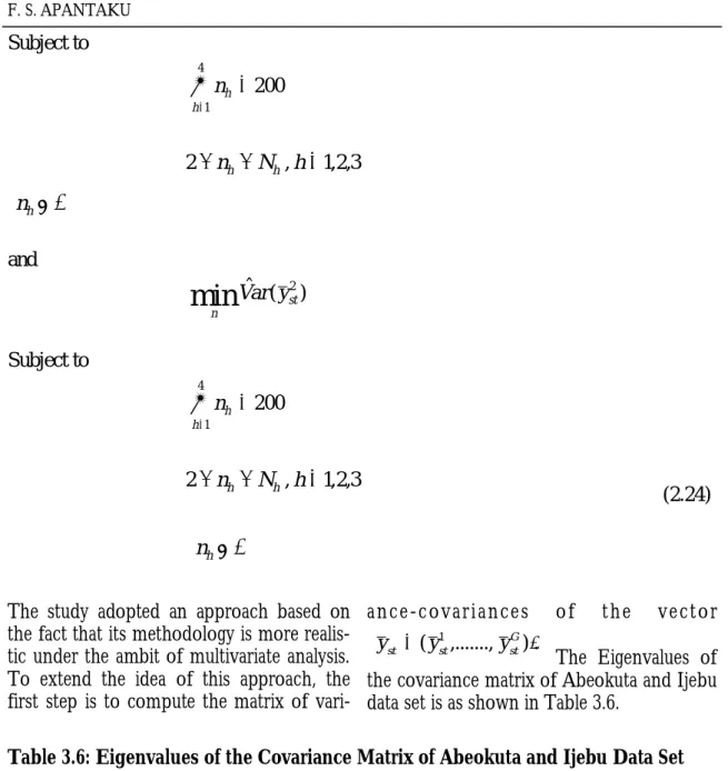
The study adopted an approach based on the fact that its methodology is more realis-tic under the ambit of multivariate analysis. To extend the idea of this approach, the first step is to compute the matrix of

vari-a n c e - c o vvari-a r i vari-a n c e s o f t h e ve c t o r The Eigenvalues of the covariance matrix of Abeokuta and Ijebu data set is as shown in Table 3.6.

. ) ,..., ( 1 

 _{st st}G

st y y

y

Subject to

and

Subject to

(2.24)





 4

1

200

h h

n

3 , 2 , 1 , 2n_h  N_h h 



h

n

) (

ˆ 2

min

st

n

y ar V





 4

1

200

h h

n

3 , 2 , 1 , 2n_h  N_h h

 

h

n

Table 3.6: Eigenvalues of the Covariance Matrix of Abeokuta and Ijebu Data Set

Eigenvalues (i)

Abeokuta Ijebu

1 0.7593 0.7788

2 0.3970 0.3391

3 0.2297 0.2089

4 0.1539 0.1266

Analysis based on principal component analysis

The principal component analysis ensured that the variance-covariance matrix was de-composed and the eigenvalues and eigen-vectors calculated from the multivariate da-ta representing information from the house-holds. The principal component on the ba-sis of the sample covariance matrix for the merged sample data sets for Abeokuta South and Ijebu North are:

with corresponding sample variance 0.7788, 0.3391, 0.2089 and 0.1266 respectively. The total variance is 1.4534 and the principal components

accounts for 53,6%, 23.3%, 14.4% and 8.7% of the total variance. Similarly, the principal components based on the merged sample correlation matrix are given by

4 3

2 1

1 0.283X 0.428X 0.278X 0.812X

Y    

4 3

2 1

2 0.069X 0.0169X 0.948X 0.309X

Y    

4 3

2 1

3 0.667X 0.729X 0.010X 0.118X

Y    

4 3

2 1

4 0.686X 0.534X 0,116X 0.481X

Y    

4 3 2 1,Y ,Y ,Y

Y   

4 3

2 1

1 1.000 0.151 0.131 0.425

~

X X

X X

Y    

4 3

2 1

2 0.151 1.000 0.211 0.505

~

X X

X X

Y    

4 3

2 1

3 0.131 0.211 1.000 0.158

~

X X

X X

Y    

4 3

2 1

4 0.425 0.505 0.158 1.000

~

X X

X X

Y    

The sample variance of the new principal components

are 1.8381, 0.9244, 0.8323 and 0.4052 re-spectively while the total variance is 4. The principal components account for 44.6%, 23.1%, 20.8% and 10.1% of the total vari-ance. Using the Eigen function, Eigen values of the merged sample covariance matrix were 0.76516, 0.36722, 0.21742 and 0.14319 with standard deviations 0.8747, 0.6060, 0.4663 and 0.3784 respectively.

CONCLUSION

In this study, optimal allocation in multi-item is developed as a multivariate optimization problem by finding the principal compo-nents. This was done by determining the overall linear combinations that concentrates the variability into few variables. It was demonstrated that the stratified samples are no longer independent. Post Stratified and Stratified Sampling approach have been pre-sented as an appropriate research design and data collection instruments.

With each unit in the population having equal chances of being chosen, the individual observations from the sample were treated as being of equal weight. Since the standard deviations of the sample strata computed differed substantially, optimum stratification was used as a method of allocating larger size samples to those strata with larger standard deviations.

From the principal component analysis, it was seen that for both Abeokuta and Ijebu data sets, the variance based on the four characteristics as multivariate is less than that of the variables when considered as a uni-variate. From the results, it was seen that there was no difference in the percentage of the total variance accounted for by the

dif-4 3 2 1,Y ,Y ,Y

ferent components from the merged sample when compared with the individual sample. The dispersion, D( ) = (X1_V-1_X)-1_σ2 which was replicated on all the characteris-tics considered, showed that optimum allo-cation was achieved when there was stratifi-cation as can be seen from the analysis.

REFERENCES

Arthanari, T.S., Dodge, Y. 1981. Mathe-matical programming on statistics. A Wiley-Interscience, Publication, John Wiley & Sons Inc.

Bankier, M. D. 1996. Estimators based on several stratified samples with applications to multiple frame survey. Journal of American Stat. Assoc. 81: 1074 – 1079.

Bethel, F. 1989. Bayes and minimax pre-diction in finite population. Journal of Statisti-cal Planning, 60, 127 – 135.

Chatterjee, S. 1972. A study of optimal allocation in multivariate stratified surveys. Skand Akt. 73, 55– 57.

Cheang, C. 2011. Sampling strategies and their advantages and disadvantages. http:// www.2.hawaii.edu/~cheang/Sampling% 20Strategies%20Advantages%20and% 20Disadvantages.htm (Accessed March 5, 2011).

Cochran, W. G. 1977. Sampling Techniques. (3rd _{Edition), New York, Wiley.}

Diaz-Garcia, J.A and Ramos-Quiroga, R. 2011. Multivariate Stratified Sampling by Stochastic Multi Objective Optimization. Xiv: 1106.0773VI. Statistical Methodology. XIV, 1116-1123.

ˆ

Diaz-Garcia, J. A., Cortez, L. U. 2008. Multivariate sampling techniques in science. Communicacion Technica: Communicaciones Del CIMAT. 8 (9), 76-83.

Diaz-Garcia, J. A., Cortez, L. U. 2006. Optimum allocation in multivariate stratified sampling: multi-objective programming. Communicacion Technica: Communicaciones Del CIMAT. 6(7), 28-33.

Diaz-Garcia, J.A., Cortez, L. U. 2008. Multi-objective optimisation for optimum allocation in multivariate stratified sampling. Survey Methodology, Vol. 34, No 2, 215-222. Hartley, H. O. 1962. Multiple frame surveys: Proceeding of the social statistics section of American Statistical Association, 205 – 215. Hartley, H. O. 1964. A new estimation the-ory for sampling surveys. Biometrics, 55, 545 – 557.

Jolliffe, I.T. 1986. Principal Component Analysis. Springer Series in Statistics. Springer Publishers.

Khan, M.G.M., Ahsan, M.J. 2003. A note on Optimum Allocation in Multivariate Stratified Sampling. South Pacific Journal Natu-ral Science, 21, 91-95.

Kish, L. 1965. Survey sampling. New York, Wiley.

Kokan, A.R and Khan, S.U., 1967. Opti-mum allocation in mutivariate surveys. An analytical solution. Journal of Royal Statistical Society. Series B, 29, 115-125.

Kolenikov, S. 2010. Re: about multi-stage strati-fied sampling designing. http://www.stata.com/ statalist/archive/2010-04/msg01453.html

(Accessed February 27, 2011).

Lumley, T. 2004. Analysis of complex survey samples. Department of Biostatistics. Univer-sity of Washington Press.

Miettinen, K. M. 1999. Non linear multi-objective optimization. Kluwer Academic Pub-lishers, Boston.

Pirzada, S., Maqbool, S. 2003. Optimal Allocation in Multivariate sampling Through Chebyshev’s Approximation. Bul-letin of the Malaysian Mathematical Science Socie-ty, 2, (26), 221 – 230.

Saxens, J., Narain, M. U., Srivastava, S. 1986. The maximum likelihood method for non-response in Surveys. Survey Methodology.

12, 50 – 62.

Sethna, B. N., Groeneveld, L. 1984. Re-search Methods in Marketing and Management. Tata, Mcgraw-Hill, publishing, New-Delhi. Steuer, R.E. 1986. Multiple criteria optimiza-tion: Theory, Computation and applications. John Wiley, New York.

Sukhatme, P.V, Sukhatme, B.V, Sukhat-me, S., Asok, C. 1984. Sampling Theory of Survey with Applications. 3rd _{Edition. Ames,} Iowa: Iowa State University Press.

Winship, C., Radbill, L. 1994. Sampling weights and regression analysis. Sociological Methods and Research, 23, (2), 230 – 257.