ISSN: 2252-8938, DOI: 10.11591/ijai.v8.i2.pp120-131 120
An improved radial basis function networks based on quantum
evolutionary algorithm for training nonlinear datasets
Lim Eng Aik1, Tan Wei Hong2, Ahmad Kadri Junoh31,3Institut Matematik Kejuruteraan, Universiti Malaysia Perlis, 02600 Arau, Perlis, Malaysia 2School of Mechatronic Engineering, Universiti Malaysia Perlis, 02600 Arau, Perlis, Malaysia
Article Info ABSTRACT
Article history: Received Dec 27, 2018 Revised Mar 29, 2019 Accepted Apr 14, 2019
In neural networks, the accuracies of its networks are mainly relying on two important factors which are the centers and spread value. Radial basis function network (RBFN) is a type of feedforward network that capable of perform nonlinear approximation on unknown dataset. It has been widely used in classification, pattern recognition, nonlinear control and image processing. Thus, with the increases in RBFN application, some problems and weakness of RBFN network is identified. Through the combination of quantum computing and RBFN provides a new research idea in design and performance improvement of RBFN system. This paper describes the theory and application of quantum computing and cloning operators, and discusses the superiority of these theories and the feasibility of their optimization algorithms.This proposed improved RBFN (I-RBFN) that combined with cloning operator and quantum computing algorithm demonstrated its ability in global search and local optimization to effectively speed up learning and provides better accuracy in prediction results. Both the algorithms that combined with RBFN optimize the centers and spread value of RBFN. The proposed I-RBFN was tested against the standard RBFN in predictions. The experimental models were tested on four literatures nonlinear function and four real-world application problems, particularly in Air pollutant problem, Biochemical Oxygen Demand (BOD) problem, Phytoplankton problem, and forex pair EURUSD. The results are compared to I-RBFN for root mean square error (RMSE) values with standard RBFN. The proposed I-RBFN yielded better results with an average improvement percentage more than 90 percent
in RMSE.
Keywords:
Evolutionary algorithm Improved RBFN Neural network Quantum computing
Radial basis function network
Copyright © 2019 Institute of Advanced Engineering and Science. All rights reserved.
Corresponding Author: Lim Eng Aik,
Institut Matematik Kejuruteraan, Universiti Malaysia Perlis, 02600 Arau, Perlis, Malaysia. Email: [email protected]
1. INTRODUCTION
The term Radial Basis Function networks (RBFN) is associated with radial basis function (RBF) in single-layered networks with structure as shown in Figure 1. Radial Basis Function Networks (RBFN) derives from the theory of function approximation. It was originally used in exact interpolation in multidimensional space by Moody and Darken [1]. RBFN displayed its advantages over other types of neural networks with better approximation abilities, simple network design and faster learning algorithms. Each year, there are a lot of finding done on RBFN, including theoretical research, algorithm design, and numerous applications in various areas such as pattern recognition, classification, prediction, control system and image processing [2-8].
RBFN are useful in approximation problems, but it is time-consuming to train the networks as it connect to a large numbers of training data, nonetheless generate high error due to possible invalid data from center selection or poor designation of spread value during training process. Although a standard RBFN has been proved by Sarimveis [2] to be faster in training using clustering algorithm for center selection and limitation with reasonable accuracy, it still produces substantial error. Such outcomes were caused by the standard RBFN that lack the ability to computes accurate spread value for network during training stage and, also the weakness pose by clustering algorithm for finding optimal center that represent the shape of distribution of given dataset. Through improving the calculation of center and spread values algorithms in standard RBFN during updating stage, we can fix the problem stated above.
Noted that the more accurate the center and spread values are assigns to the network, the more accurate the information that feeds to the output layer of network, resulting in accurate results. In this paper, an improved RBFN (I-RBFN) that outperforms the standard RBFN in term of accuracies is presented. The proposed I-RBFN used quantum computing combined with evolutionary algorithm to optimize the algorithm of RBFN.The proposed networks efficiency is demonstrated through the application of eight experimental models, with four nonlinear model from literatures, three real-world problems data obtained from Lim [9] and one real-world time-series data from XM metatrader 4 trading platform [10]. The advantages of the presented proposed networks are identified and the results are compared with standard RBFN and discussed.
Figure 1. The architecture of RBFN
2. RELATED WORKS
Radial basis function networks (RBFN) are well-known for its ability to generalize and approximate a sample data without the requirement for the equation and coefficients, particularly when an unknown model describing an unknown complex relation with abundant training data. Due to their ability to generalize substantially, RBFN are usually selected for this purpose [11-23]. Furthermore, in this big data era, many domains such as image processing, text categorization, biometric, microarray, etc. had the size of datasets so large, that real-time system requires long time and memory storage to process them. Under the same group, the backpropagation neural networks also can generalize and approximate complex dataset. However, due to the architecture of backpropagation neural networks that works in forward and backward direction, delays in training time is unavoidable. Furthermore, in term of approximation, multiple literatures showed that the RBFN is more superior than backpropagation neural networks, in term of training speed and accuracy [24-28].
Two main criteria that determine the accuracy of an RBFN are the initial center and spread value. In this paper, we focus on criteria and perform adjustment on it by using hybrid learning from quantum algorithm and evolutionary algorithm, with these algorithm incorporated into RBFN. Throughout many literatures, we found that obtaining optimal center in RBFN play vital role in determine its accuracy in approximation problem [3-4], [29-42]. Moreover, recent research by Neill et al. [43] proof the supremacy of quantum algorithm combining with machine learning in performing computation for large dataset that beyond capabilities of most classical optimization algorithm. The ability of quantum algorithm is further supported Gao et al. [44] that proof quantum algorithm combined with RBFN in solving big data classification problem. Early literatures also had shown the capability of quantum algorithm in solving complicated linear systems [45-46] and unknown eigenvalues problem [47]. A combination of quantum
algorithm with evolutionary algorithm proof to obtained significant improvement in results by ensuring the diversity in initial search of data as shown by Chung et al. [48] and Zhang et al. [49] in compared to standard evolutionary algorithm itself. Shang et al. [50] and Basu [51] demonstrated using quantum clonal algorithm with evolutionary algorithm in solving multi-objectives problem and yield significant improvement compared to standard evolutionary algorithm. The ability of quantum algorithm were supported by recent literatures by Biamonte et al. [52] and Godfri et al. [53] that stated the hybrid of quantum algorithm with machine learning such as neural networks outperform classical machine learning algorithm in term of searching, optimizing, simulating and solving complicated system. In the same year, Silveira and Vellasco [54] proposed a new quantum-inspired evolutionary algorithm for solving combinatorial and numerical optimization problems, providing better results than classical genetic algorithm with less computational effort. Similar idea in quantum-inspired evolutionary algorithm is also proposed by Ozsoydan and Baykasoglu [55] using quantum firefly algorithm for overcoming the local minima problem in classical firefly algorithm.
In solving the weakness of neural networks in center selection, obtaining optimal weight and spread value, many literatures proposed the applications of hybrid neural network using evolutionary algorithm. In finding solution to obtained better weights adjustment and gaining accurate approximation, Navarro et al. [56, 57] demonstrated that the hybrid of evolutionary algorithm such as particle swarm optimization (PSO) with RBFN shows a good performance in classification problems and approximation problems. This work is extended by Leung et al. [58] by introducing a novel PSO method or adjusting the RBFN networks weight. Similar work on evolutionary algorithm hybrid with RBFN was found in Chang et al. [59] that focus on center adjustment. The applications of evolutionary algorithm combine with RBFN were then extended to using genetic algorithm with RBFN [31], [60-61], joining two evolutionary algorithm for better performance such as genetic algorithm join with PSO [3], [62], and modified PSO with RBFN [11]. The used of evolutionary algorithm as a tool for obtaining optimal center, weight and spread values in RBFN training was indeed a good method if the networks training speed and computation cost are not main concerns.
In the mentioned literatures, clearly most approaches focus in either using evolutionary algorithm with RBFN or, quantum algorithm with evolutionary algorithm. Furthermore, many approaches focus on applying separate part of methods or algorithm for weight adjustment instead of focusing on obtaining optimal center value and spread value for improving RBFN results. In this paper, we focus on improving the RBFN algorithm for better center selection and spread value which in turn making RBFN algorithm precede the computation with better accuracy. This paper is organized with the following section describing the standard RBFN, follows by steps in improving the standard RBFN by including quantum algorithm and evolutionary algorithm into RBFN algorithm. Then, in section 4 discussed the simulation results of each models and compared with standard RBFN for accuracies. Finally, section 5 concludes the findings and discussed some future work that would help in improving the proposed improved RBFN.
3. METHODOLOGY
3.1. Radial basis function network (RBFN)
RBFN is an intelligent interpolation technique for modeling a linear or nonlinear multidimensional data. RBFN is often used for prediction problems. Its kernel has two parameters; the center and its radius. These two parameters can determined through unsupervised or supervised learning as proposed by Moody and Darken in 1989 [1]. RBFN is a type of feed-forward neural network. The network structure consists of three-layer network similar to multi-layer feed-forward network. In the network structure of RBFN as shown in Figure 1, the first layer is the input layer and is composed of signal source nodes. The second layer is a hidden layer, and the number of nodes of the layer is determined by the nature of the problem to be solved and the characteristics of the specific problem. The transfer function of the neurons in this layer is the radial basis function, which is a global function that responses as the forward network transformation function. The third layer is the output layer, which responds to the input layer.
The main idea of the RBFN is to use the radial basis function as the "base" of the hidden layer unit to build the hidden layer. In the hidden layer, the input vector is transformed. Thus, low-dimensional input data can convert to a high-dimensional space. Such approach can transform a linearly inseparable problem in a low-dimensional space into a linearly separable in a high-dimensional space, thereby solving the related problem. RBFN training is simple and has fast learning convergence. It can approximate any nonlinear function. Therefore, the RBFN has a extensive applications in pattern recognition, image processing, predictions and nonlinear control. From the perspective of function approximation, RBFN are local approximations. If the number of neural units in the hidden layer reaches a certain level, the network can approximate any continuous function with arbitrary precision. In addition, due to RBFN adopts a linear mapping relationship between the output layer and the hidden layer; the network can avoid the complicated
back-propagation operation as in back-propagation neural network. Therefore, in RBFN, the speed of operation and the accuracy of nonlinear fitting are improved. During the operation to solve a problem, the RBFN has the characteristics of the training samples corresponding to the radial basis function mapping, resulting in a large amount of network computation, and may cause problems in solving the networks weights.
3.2. RBFN model and learning algorithm
RBFN by default uses the Gaussian function as the kernel function of the hidden unit, see (1).
2
2
i ik i
k
X C
k
r e
(1)
Where rk is the output value of the k-th Gaussian unit of the hidden layer; C is the i-th input variable value of the center of the kernel of the k-th Gaussian unit; k is the spread of the kernel of the k-th Gaussian unit.
The supervised learning rule used to adjust the link weighting value between the hidden unit and the output unit, and the threshold value of the output unit. The difficulty with RBFN determines the number of hidden units and the center of the Gaussian function and the radius parameters. The two parameters, center and radius, can determined by supervised or unsupervised learning. The supervised learning of RBFN is similar to back-propagation, and the learning rules can derived by minimizing the sum of squares errors and the steepest descent method. Unsupervised learning uses the K-means algorithm to find the cluster center of the sample as the center of the Gaussian function of each hidden unit. Though RBFN has a many applications in pattern recognition, predictions, and control system, the algorithms still a disadvantage on independent variables have the same position, so the optimal centers can determined. However, each independent variable has different influence on the dependent variable, thus affecting the spread value of network during training process.
3.3. RBFN implementation, advantages and limitation
The implementation of the RBF neural network consists of two parts: the network structure part and the algorithm parameter part. The network structure is designed to determine the number of nodes in the hidden layer of the network. The part of the algorithm parameters is determined for the three important parameters of the data center of the radial basis function, the spread constant and the output layer weight. Since the number of hidden layer nodes is consistent with the number of samples, and the center of the radial basis function is the sample itself, only the spread constant and the output layer weight need to be determined when establishing the network. However, when building an RBFN, the learning algorithm needs to solve more problems, including the determination of the number of hidden layer nodes, the determination of the data center of the radial basis function, the spread constant, and the correction of the weights of the output layer.
The establishment and training of the radial basis function neural network is composed of two stages. The first phase primarily determines the data center of the radial basis function in the hidden layer, typically used as the centers self-organizing selection method for unsupervised learning processes. The input samples are clustered to determine the center of the radial basis function of the hidden layer nodes. The RBFN has its adaptive ability and fault tolerance. Therefore, while dealing with the complex evaluation of nonlinearity, the factors that have no significant influence on the evaluation results can effectively eliminated. The RBFN is improved via the supervised learning rules used to adjust the spread value of the network and, applying center selection algorithm for obtaining optimal centers. The learning rule is derived by minimizing the sum of squared errors and the steepest descent method.
3.4. Quantum evolutionary algorithm (QEA)
Classical evolutionary algorithms (EA) do not take advantage of the information provided by immature subgroups in evolution, thus limiting the rate of evolution. Therefore, by introducing a good guiding mechanism in evolution can enhance the intelligence of the algorithm, improve the search efficiency, and solve the problem of premature convergence and convergence speed in EA. Many improvements to the existing EA are also devoted to this aspect. Quantum Evolutionary Algorithm (QEA) is an evolutionary algorithm that combines evolutionary algorithms with quantum theory. QEA is based on the concepts and theories of quantum computing such as qubit, which is a type of quantum bits, to encode chromosome. The representation of the probability amplitude can make a quantum chromosome simultaneously represent the information of multiple states, bringing a rich population, and the information of the current optimal
individual that can easily use to guide the mutation, so the population evolves toward the good model with a high probability and accelerate algorithm convergence.
3.4.1. The concept of QEA
In QEA, the smallest unit of information is a qubit. The state of a qubit can take 0 or 1, and its state can expressed as
0 1
(2)
whereand are two complex numbers representing the probability of occurrence of the corresponding state 2 2 1 ; 2 and 2 represents the probability that a quantum bit is in state 0 and state 1, respectively. The coding methods commonly used in evolutionary algorithms are binary coding, decimal coding, and symbol coding. In QEA, a novel qubit-based coding scheme is used, which is a quantum bit is defined by a pair of complex numbers. A system with m-qubits can described as
1 2
1 2
m
m
(3)where 2 2 1, i1, 2, ..., .m This representation can characterize any linear superposition state. 3.4.2 QEA algorithm
Classical QEA is a probabilistic algorithm similar to evolutionary algorithms. The chromosome population in the t-th generation is Q t
q q q1t, 2t, 3t, ...,qtn
, where n is the population size, t is the evolutionary variable, and qtjis the chromosome defined as follows1 2
1 2
, 1, 2, ..., , where is chromosome length t
t t
t m
j t t t
m
q j n m
. (4)The difference between QEA and EA is only the two steps of "generating P(t) from Q(t)" and "updating Q(t)". In the "initialized population Q(t)", ifmt,
t m
and all qtjin Q(t) are initialized to1 2, it means that all possible linear superposition states appear with the same probability; In the step of "generating P(t) from Q(t)", by observing the state of Q(t), a set of ordinary solutions P(t) is generated, where in the t-th generation ( )
1, 2, ...,
t t t
n
P t x x x , each xtj
j1, 2, ...,m
has the length of the string of m
x x1, 2,...,xm
, which is obtained by the quantum bit amplitude t 2i
or t 2 i
i1, 2,...,m
. The process corresponding to the binary case is to randomly generate a [0, 1] number. If it is greater than2
t i
, take 1; otherwise, take 0.
In the step of "updating Q(t)", it is possible to use the traditional cross-over and variation, or to use some suitable quantum gate transforms to generate Q(t) according to the superposition characteristics of quantum bits and the theory of quantum transition. Note that due to the requirement of probability normalization conditions, the quantum gate transformation matrix must be a reversible unitary matrix, which needs to satisfy U U* UU*
U* is a conjugate tranpose of U
. The commonly used quantum transformation matrices are the XOR gates, controlled XOR gates, revolving gates and Hadamard gates.For quantum mutation strategy, there are two options available.
Mutation strategy 1: Mutation operation is a method of generating new individuals in EA. The usual mutation operation is a random variation. The evolution of individuals has random disturbance factors, and the existing information available in evolution is not utilized. Therefore, the convergence speed is slow. The following discusses a simple method of quantum chromosome variation, which can effectively use contemporary information, and derive the probability distribution of a quantum chromosome from the current optimal solution, which is somewhat similar to the probability genetic algorithm, but the operation process is much simpler. The specific process is described as the introduction of a guide quantum chromosome by
the optimal individual obtained from the current evolutionary operation, and randomly distributes the quantum chromosome around it as the next-generation quantum population, which is described by the formula as
_
1
1 _
guide current best current best
Q t a p t a p t (5)
1
guide
0,1Q t Q t b normrnd (6)
wherepcurrent_best
t is the optimal individual obtained until evolution to the t-th generation,Qguide
t is the guiding quantum chromosome, a is the guiding factor for the quantum chromosome, and b is the difference of the random dispersion of the quantum population. Obviously, using the observation method in the above algorithm, in order to obtain the chromosome P
1 1 0 0 1 ,
just make the quantum chromosome Q as
0 0 1 1 0 , where
QP. If P is the optimal solution in the search space, the closer the quantum chromosome in the population is to Q, the greater the probability of getting the optimal solution.The smaller the value of a, the greater the influence of quantum populationQguide. When a = 0,
,
guide
Q P after observation Qguide, P is obtained with probability 1. When a = 1/2, Qguide has no effect on observation. Generally a and b take the range of a ∈ [0.1, 0.5], b ∈ [0.05, 0.15].
Mutation strategy 2: In quantum theory, the transition between states is achieved by a quantum gate transformation matrix, which reveals: the rotation angle of the quantum revolving gate can also be used to characterize the mutation operation in the quantum chromosome, then it is convenient to add the information of the optimal individual to the variation and accelerate the convergence of the algorithm. In the problem of 0, 1 coding, the following quantum mutation operator is designed to accelerate evolution,
cos sinsin cos
U
(7)In (7) represents a quantum revolving gate, where xi is the i-th bit of the current chromosome; besti is the i-th bit of the current optimal chromosome; f
x is the fitness function, i is the magnitude of the rotation angle which control the speed of algorithm convergence; s
i i
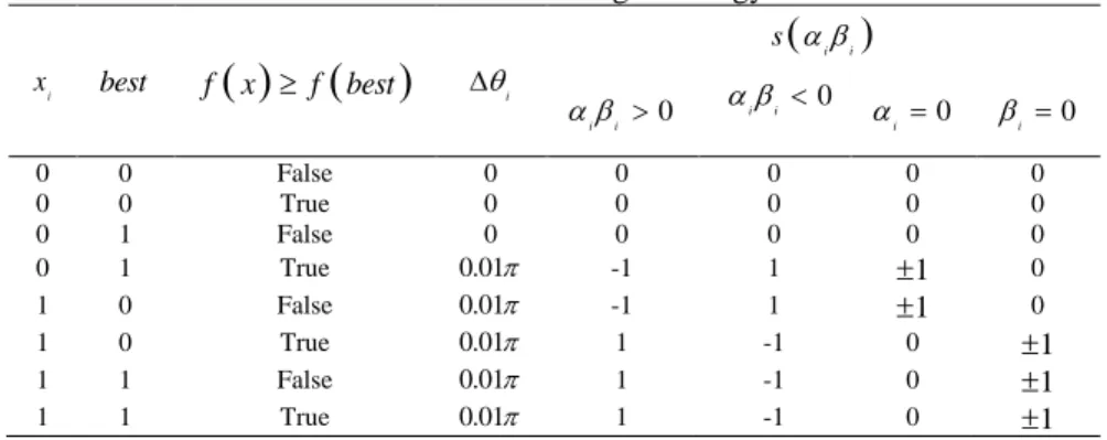
is the direction of the rotation angle to ensure the convergence of the algorithm. Why does this rotating quantum gate ensure that the algorithm quickly converges to a chromosome with higher fitness? Table 1 shows the construction of a rotating quantum gate.Table 1. Rotation angle strategy
i
x best f x
f best
i
i i
s
0
i i
i i 0 0 i
i 0
0 0 False 0 0 0 0 0
0 0 True 0 0 0 0 0
0 1 False 0 0 0 0 0
0 1 True 0.01 -1 1 1 0
1 0 False 0.01 -1 1 1 0
1 0 True 0.01 1 -1 0 1
1 1 False 0.01 1 -1 0 1
1 1 True 0.01 1 -1 0 1
For example, whenxi 0, besti 1, f x
f best
, in order to converge the current solution to a chromosome with higher fitness, the probability of the current solution 0 should increase, to tunei 2 becomes larger, then if
i, i
is in the first and third quadrants, it should rotated clockwise; if
i, i
isin the second and fourth quadrants, θ rotates counterclockwise, as shown in Figure 2. The rotation transformation described above is only one of the quantum transformations. Different quantum transformations can use for different problems and it is also possible to design its own unitary transformation as needed. For non-binary coding problems, different observation methods are constructed, and the generation of the variation angle is similar to this, and will not be discussed in detail here.
Figure 2. Rotation transformation diagram
3.4.3 QEA-RBFN algorithm
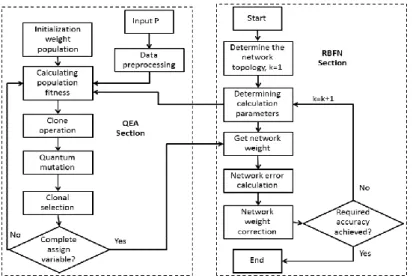
The steps of the QEA algorithm can described as follows: Step 1: Initialize evolutionary variable, t0.
Step 2: Initialize seed community, Q t
, with initially equal probability of 1 2 t i ;
Step 3: Generate P(t) from Q(t) (different coding modes adopt different observation modes, wherein the algorithm uses binary coding and observes in the above manner);
Step 4: Evaluate the affinity of the population P(t), save the optimal solution;
Step 5: Checking stopping criteria, when the stopping criteria is met, the current optimal individual is the output, the algorithm stops, otherwise, continues;
Step 6: Cloning Q(t) generates Q'(t);
Step 7: Perform a quantum mutation strategy 2 on Q'(t) to generate Q"(t);
Step 8: Generating a new individual Q(t) by selecting compression Q"(t), t = t +1, go to step3.
The flow chart of the implementation of the RBFN based on the QEA optimization is given below, as shown in Figure 3.
4. RESULTS AND DISCUSSION
The proposed I-RBFN was tested using 4 nonlinear function from literatures, which are Santner et al. [63] function given in (8), Lim et al. [64] function in (9), Dette and Pepelyshev [65] function in (10), and Friedman [66] function in (11). For all these 4 functions, the training set for RBFN consists of 400 sets of random generated data points and test set comprises 400 sets of random generated data points, both in range of [0,1].
( ) exp( 1.4 ) cos(3.5 ), 0,1f x x x x (8)
1
1
2
130 5 sin 5 4 exp 5 100 , 0,1 , 1, 2.
6 i
f x x x x x i (9)
2
2
2
2
1 2 2 2 3 3
4 2 8 8 3 4 16 1 2 1 , i 0,1 , 1, 2, 3.
f x x x x x x x x i (10)
2
1 2 3 4 5
10 sin 20 0.5 10 5 , i 0,1 , 1, 2, 3, 4, 5.
f x x x x x x x i (11)
I-RBFN was also tested on 4 real-world datasets for its performance. The Biochemical Oxygen Demand (BOD) concentration dataset, phytoplankton growth rate and death rate dataset and air pollutant dataset were obtained from Aik and Zainuddin [67]. Another which is the dataset from forex for EURUSD pairs is collected from XM Metatrader 4 database [10]. The BOD dataset and phytoplankton dataset both consists of 100 sets of data and the test set comprises 100 sets of data. Meanwhile, for air pollutant dataset, the training set has 480 sets of data and the test set has 72 sets of data, which both were taken from hourly air data. For EURUSD pairs, the training set consists of 519 sets of data taken from year 2016 to end of year 2017. The test set consists of 155 sets of data taken from January year 2018 to August 2018.
The experiment was implemented by using the newrb function because it represents the general form of an RBFN. Furthermore, the proposed I-RBFN has been implemented by using MATLAB’s function. Gaussian basis function has been used for both networks with other parameters such as spread was set to default value, so the performance of the proposed network can evaluated effectively [8]. Performance of standard RBFN and I-RBFN in this experiment has been measured by comparing the computation time taken for training with number of iteration taken for convergence and the Root Mean Squared Error (RMSE) to measure how well both networks approximates the chosen functions and it is given by:
2 11 n
i i
i
RMSE O P
n
where n is the number of predicted responder; Oi is the target value for time-step i, and Pi is the predicted value of the model at time-step i.
The number of centers for RBFN is fixed to 10 centers for all 8 datasets training. For air pollutant problem, the pollutant monitored includes carbon monoxide, nitric oxide, nitrogen dioxide, ozone, and oxides of nitrogen. For experimental purposes, hourly updated air quality data obtained from Aik and Zainuddin [67] has been used to predict the trend of interested pollutants for Nitric Oxide, Nitrogen Dioxide and Oxides of Nitrogen. While for Phytoplankton problem, growth rate and death rate have been used as the interested values. As for the BOD problem, the BOD concentration has been taken as the interested value. Finally, the forex EURUSD dataset consists of three variables is taken considered for training, which are the daily highest price, daily lowest price and open price, while the close price is used for prediction.
Results from Table 2 shows that I-RBFN networks outperform standard RBFN in average RMSE and standard deviation of RMSE. All results of average RMSE in Table 2 are calculated using ten times run of each networks. From Table 2, I-RBFN network surpasses the standard RBFN in accuracy and network architecture by using training set which consists only 81.8%, 71.8%, 68.5%, and 65.8% of total dataset size for Santner dataset, Lim dataset, Dette dataset, and Friedman dataset, respectively. While I-RBFN network training for real-world dataset involves the BOD dataset, Phytoplankton dataset, Air pollutant dataset and forex EURUSD dataset used only 81.8%, 71.8%, 68.5% and 66.8%, respectively. This means that, it is possible to suitable number of dataset such that, it will provide a network with reduced complexity, faster training time and improved accuracy. Table 3 shows the results of the percentage of improvement of RMSE for I-RBFN network in compared to standard RBFN. Results showed that I-RBFN network outperform
standard RBFN network in term of accuracy more than 95% for Santner dataset, Lim dataset, Dette dataset, BOD dataset, phytoplankton dataset and air pollutant dataset. Meanwhile, for Friedman dataset gain 93.45% improvement, and EURUSD dataset obtained 92.41% improvement over standard RBFN. Therefore, I-RBFN showed significant improvement over standard RBFN with average percentage more than 95% even for dataset with high nonlinearity.
Table 2. Performance of I-RBFN and Standard RBFN prediction results for datasets
Dataset
Standard RBFN I-RBFN
Average of RMSE Standard Deviation
of RMSE Average of RMSE
Standard Deviation of RMSE
Santner 0.160980 0.132510 3.58E-15 2.61E-15
Lim 0.151190 0.053404 4.88E-15 3.82E-16
Dette 1.938260 1.318204 2.07E-05 2.96E-05
Friedman 1.333590 0.700492 0.087283 0.061549
BOD 0.000252 3.87e-07 5.07E-15 3.38E-15
Phytoplankton 0.004980 0.000933 2.25E-15 1.91E-15
Air Pollutant 4.203630 2.860265 0.027499 0.010795
EURUSD 0.031649 0.004812 0.002400 0.000124
Table 3. Percentage of improvement for I-RBFN over standard RBFN by RMSE
Dataset Percentage of Improvement (%)
Santner 100.00
Lim 100.00
Dette 99.99
Friedman 93.45
BOD 100.00
Phytoplankton 100.00
Air Pollutant 99.34
EURUSD 92.41
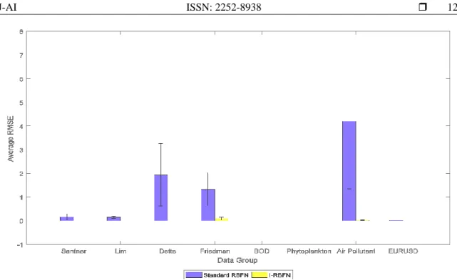
The results Friedman dataset and forex EURUSD dataset showed improvement less than 95% compared to others dataset. Both of this datasets are highly nonlinear data. Possible existence of additional factor that is not included in dataset possibly is the reason behind the low improvement percentage occurs for Friedman dataset. Additionally, for forex EURUSD dataset, the low improvement percentage is due to many possible factors not included in the dataset that also drives the movement of this currency values. Factor that cannot be quantified, such as political influences or natural disaster, can affect the currency fluctuation. Hence, if such factors can quantify and includes in the dataset, improvement in percentage is expected. From Table 2 and Table 3, we observed that I-RBFN network provide such consistent results even that it uses less dataset and still able to perform such satisfying results. The results of prediction from I-RBFN network are consistent as we observed from Table 1, the standard deviation of RMSE was much lower than standard RBFN. Figure 4 shows the error bar plot that displayed the comparison of errors for both the networks. Clearly, the standard RBFN has larger error in compared to I-RBFN network for all datasets.
The I-RBFN network and Standard RBFN performed well in the experiments for dataset with smaller range that lies in [0,1]. However, for larger range of dataset such as air pollutant dataset, the standard RBFN performed poorly in accuracy. Besides, the I-RBFN network is superior in accuracies but a proper adjustment in the network centers and spread value can enhance the networks accuracy to much higher level. The results in Table 1 shows that even with less dataset used for training, if the right centers and spread value are assigned, can impact in prediction accuracy. The uses of huge number of dataset does not always guarantee the desirable prediction accuracies, but sufficient number of dataset that can represent the shape of the distribution for the dataset is enough for providing good prediction results. Furthermore, a large number of training dataset might contain invalid data that could jeopardize the desired accuracy, not mentioning the size of network it would create and the time taken for training.
Hence, there is no denial on the ability of the I-RBFN network and standard RBFN in prediction, but it comes with a hefty compensation for the accuracy if the proper value of networks centers and spread value are not assigned. As the number of datasets for the network becomes lesser and it results in much simpler network architecture and possibly free of invalid dataset. Although both models provide satisfying results, the network structure and accuracy of the I-RBFN network is superior compared to the standard RBFN network.
Figure 4. Error Bar Plot for datasets using standard RBFN and I-RBFN
5. CONCLUSION
Four literatures nonlinear functions and four real-world problems have been simulated in this paper, where we applied for real-world problems on prediction of BOD problem, phytoplankton problem, air pollution problem and forex EURUSD price prediction problem. The performance of both networks has been compared to the case using the Root Mean Squared Error (RMSE) and standard deviation as the criteria for performance measurement and network prediction consistency. Results from all eight studies showed that the I-RBFN network is far better than the standard RBFN in prediction accuracy and network architecture. Thus, it is possible to improve the accuracy of the proposed network by using clustering methods to choose the best value of number of center to be used for different type of dataset. As conclusion, the proposed I-RBFN is far superior to the standard I-RBFN network as for network accuracy. Since self-organized selection of centers can performed by clustering algorithms for selecting significant centers, sufficient to represent the distribution of dataset for the hidden nodes, it would be interesting if the networks is test with high noise training data with clustering algorithm such as K-means algorithm, or fuzzy C-means algorithm as center selector to verify the efficiency of the I-RBFN.
REFERENCES
[1] J. Moody and C. J. Darken, “Moody, J., & Darken, C. J. (1989). Fast learning in networks of locally-tuned processing units. Neural Computation, 1, 281-294.,” Neural Comput., vol. 1, pp. 281–294, 1989.
[2] H. Sarimveis, A. Alexandridis, and G. Bafas, “A fast training algorithm for RBF networks based on subtractive clustering,” Neurocomputing, vol. 51, pp. 501–505, 2003.
[3] A. Alexandridis, E. Chondrodima, N. Giannopoulos, and H. Sarimveis, “A Fast and Efficient Method for Training Categorical Radial Basis Function Networks,” IEEE Trans. Neural Networks Learn. Syst., pp. 1–6, 2016.
[4] A. Alexandridis, E. Chondrodima, N. Giannopoulos, and H. Sarimveis, “A fast and efficient method for training categorical radial basis function networks,” IEEE Trans. Neural Networks Learn. Syst., vol. 28, no. 11, pp. 2831– 2836, 2017.
[5] Y. Hu, J. J. You, J. N. K. Liu, and T. He, “An eigenvector based center selection for fast training scheme of RBFNN,” Inf. Sci. (Ny)., vol. 428, pp. 62–75, 2018.
[6] E. M. da Silva, R. D. Maia, and C. D. Cabacinha, “Bee-inspired RBF network for volume estimation of individual trees,” Comput. Electron. Agric., vol. 152, pp. 401–408, 2018.
[7] D. Shan and X. Xu, “Multi-label Learning Model Based on Multi-label Radial Basis Function Neural Network and Regularized Extreme Learning Machine,” Moshi Shibie yu Rengong Zhineng/Pattern Recognit. Artif. Intell., vol. 30, no. 9, 2017.
[8] Y. Sun et al., “The application of RBF neural network based on ant colony clustering algorithm to pressure sensor,” Chinese J. Sensors Actuators, vol. 26, no. 6, 2013.
[9] L. E. Aik, “Modified Clustering Algorithms for Radial Basis Function Networks,” Universiti Sains Malaysia, 2006. [10] L. XM Global, “XM Metatrader 4,” 2018. [Online]. Available: https://www.xm.com/mt4. [Accessed: 20-Jul-2018].
[11] S. Mirjalili, “Evolutionary Radial Basis Function Networks,” in Studies in Computational Intelligence, 2019, pp. 105–139.
[12] A. Osmanović, S. Halilović, L. A. Ilah, A. Fojnica, and Z. Gromilić, “Machine learning techniques for classification of breast cancer,” in IFMBE Proceedings, 2019.
[13] Y. Lei, L. Ding, and W. Zhang, “Generalization Performance of Radial Basis Function Networks,” Neural Networks Learn. Syst. IEEE Trans., vol. 26, no. 3, pp. 551–564, 2015.
[14] C. Arteaga and I. Marrero, “Universal approximation by radial basis function networks of Delsarte translates,”
Neural Networks, vol. 46, pp. 299–305, 2013.
[15] S. Lin, “Linear and nonlinear approximation of spherical radial basis function networks ✩,” vol. 35, pp. 86–101, 2016.
[16] M. Mohammadi, A. Krishna, S. Nalesh, and S. K. Nandy, “A Hardware Architecture for Radial Basis Function Neural Network Classifier,” IEEE Trans. Parallel Distrib. Syst., 2018.
[17] M. W. L. Moreira, J. J. P. C. Rodrigues, N. Kumar, J. Al-Muhtadi, and V. Korotaev, “Evolutionary radial basis function network for gestational diabetes data analytics,” J. Comput. Sci., 2018.
[18] K. Kavaklioglu, M. F. Koseoglu, and O. Caliskan, “International Journal of Heat and Mass Transfer Experimental investigation and radial basis function network modeling of direct evaporative cooling systems,” Int. J. Heat Mass Transf., vol. 126, pp. 139–150, 2018.
[19] M. Smolik, V. Skala, and Z. Majdisova, “Advances in Engineering Software Vector fi eld radial basis function approximation,” Adv. Eng. Softw., vol. 123, no. 17, pp. 117–129, 2018.
[20] Y. Li, X. Wang, S. Sun, X. Ma, and G. Lu, “Forecasting short-term subway passenger flow under special events scenarios using multiscale radial basis function networks,” Transp. Res. Part C Emerg. Technol., 2017.
[21] G. W. Chang, H. J. Lu, Y. R. Chang, and Y. D. Lee, “An improved neural network-based approach for short-term wind speed and power forecast,” Renew. Energy, 2017.
[22] Q. P. Ha, H. Wahid, H. Duc, and M. Azzi, “Enhanced radial basis function neural networks for ozone level estimation,” Neurocomputing, 2015.
[23] Z. Majdisova and V. Skala, “Radial basis function approximations : comparison and applications,” Appl. Math. Model., vol. 51, pp. 728–743, 2017.
[24] F. Mateo, R. Gadea, E. M. Mateo, and M. Jiménez, “Multilayer perceptron neural networks and radial-basis function networks as tools to forecast accumulation of deoxynivalenol in barley seeds contaminated with Fusarium culmorum,” Food Control, 2011.
[25] D. Seyed Javan, H. Rajabi Mashhadi, and M. Rouhani, “A fast static security assessment method based on radial basis function neural networks using enhanced clustering,” Int. J. Electr. Power Energy Syst., 2013.
[26] M. Zounemat-Kermani, O. Kisi, and T. Rajaee, “Performance of radial basis and LM-feed forward artificial neural networks for predicting daily watershed runoff,” Appl. Soft Comput. J., 2013.
[27] H. Shafizadeh-Moghadam, J. Hagenauer, M. Farajzadeh, and M. Helbich, “Performance analysis of radial basis function networks and multi-layer perceptron networks in modeling urban change: a case study,” Int. J. Geogr. Inf. Sci., 2015.
[28] M. Bagheri, S. A. Mirbagheri, M. Ehteshami, and Z. Bagheri, “Modeling of a sequencing batch reactor treating municipal wastewater using multi-layer perceptron and radial basis function artificial neural networks,” Process Saf. Environ. Prot., 2015.
[29] D. K. S. Tok, D. L. Yu, C. Mathews, D. Y. Zhao, and Q. M. Zhu, “Adaptive structure radial basis function network model for processes with operating region migration,” Neurocomputing, 2015.
[30] D. P. Ferreira Cruz, R. Dourado Maia, L. A. da Silva, and L. N. de Castro, “BeeRBF: A bee-inspired data clustering approach to design RBF neural network classifiers,” Neurocomputing, 2016.
[31] W. Jia, D. Zhao, T. Shen, C. Su, C. Hu, and Y. Zhao, “A new optimized GA-RBF neural network algorithm,”
Comput. Intell. Neurosci., 2014.
[32] W. Jia, D. Zhao, and L. Ding, “An optimized RBF neural network algorithm based on partial least squares and genetic algorithm for classification of small sample,” Appl. Soft Comput. J., 2016.
[33] C. Sbarufatti, M. Corbetta, M. Giglio, and F. Cadini, “Adaptive prognosis of lithium-ion batteries based on the combination of particle filters and radial basis function neural networks,” J. Power Sources, 2017.
[34] F. Abbas and M. C. Babahenini, “Gaussian Radial Basis Function for Efficient Computation of Forest Indirect Illumination,” 3D Res., 2018.
[35] N. Benoudjit and M. Verleysen, “On the kernel widths in radial-basis function networks,” Neural Process. Lett., 2003.
[36] A. A. K.S. Kasiviswanathan, “Radial Basis Function Artificial Neural Network: Spread Selection,” Int. J. Adv. Comput. Sci., 2012.
[37] R. Hartley and S. B. Kang, “Parameter-free radial distortion correction with center of distortion estimation,” IEEE Trans. Pattern Anal. Mach. Intell., 2007.
[38] D. Wettschereck and T. Dietterich, “Improving the Performance of Radial Basis Function Networks by Learning Center Locations,” Adv. Neural Inf. Process. Syst., 2012.
[39] Siraj-Ul-Islam, R. Vertnik, and B. Šarler, “Local radial basis function collocation method along with explicit time stepping for hyperbolic partial differential equations,” Appl. Numer. Math., 2013.
[40] D. Guo, Y. Zhang, Q. Xiang, and Z. Li, “Improved radio frequency identification indoor localization method via radial basis function neural network,” Math. Probl. Eng., 2014.
Neurocomputing, 2015.
[42] M. Alsalamah, S. Amin, and J. Halloran, “Diagnosis of heart disease by using a radial basis function network classification technique on patients’ medical records,” in Conference Proceedings - 2014 IEEE MTT-S International Microwave Workshop Series on: RF and Wireless Technologies for Biomedical and Healthcare Applications, IMWS-Bio 2014, 2015.
[43] C. Neill et al., “A blueprint for demonstrating quantum supremacy with superconducting qubits,” Science (80-. )., 2018.
[44] J. Gao et al., “Experimental Machine Learning of Quantum States,” Phys. Rev. Lett., 2018.
[45] B. D. Clader, B. C. Jacobs, and C. R. Sprouse, “Preconditioned quantum linear system algorithm,” Phys. Rev. Lett., 2013.
[46] X. D. Cai et al., “Experimental quantum computing to solve systems of linear equations,” Phys. Rev. Lett., 2013. [47] X. Q. Zhou, P. Kalasuwan, T. C. Ralph, and J. L. O’brien, “Calculating unknown eigenvalues with a quantum
algorithm,” Nat. Photonics, 2013.
[48] C. Y. Chung, H. Yu, and K. P. Wong, “An advanced quantum-inspired evolutionary algorithm for unit commitment,” IEEE Trans. Power Syst., 2011.
[49] G. Zhang, “Quantum-inspired evolutionary algorithms: A survey and empirical study,” J. Heuristics, 2011. [50] R. Shang, L. Jiao, F. Liu, and W. Ma, “A novel immune clonal algorithm for MO problems,” IEEE Trans. Evol.
Comput., 2012.
[51] M. Basu, “Artificial immune system for combined heat and power economic dispatch,” Int. J. Electr. Power Energy Syst., 2012.
[52] J. Biamonte, P. Wittek, N. Pancotti, P. Rebentrost, N. Wiebe, and S. Lloyd, “Quantum machine learning,” Nature. 2017.
[53] C. Godfrin et al., “Operating Quantum States in Single Magnetic Molecules: Implementation of Grover’s Quantum Algorithm,” Phys. Rev. Lett., 2017.
[54] L. R. da Silveira, R. Tanscheit, and M. M. B. R. Vellasco, “Quantum inspired evolutionary algorithm for ordering problems,” Expert Syst. Appl., 2017.
[55] F. B. Ozsoydan and A. Baykasoğlu, “Quantum firefly swarms for multimodal dynamic optimization problems,”
Expert Syst. Appl., 2019.
[56] F. Fernández-Navarro, C. Hervás-Martínez, J. Sanchez-Monedero, and P. A. Gutiérrez, “MELM-GRBF: A modified version of the extreme learning machine for generalized radial basis function neural networks,”
Neurocomputing, 2011.
[57] F. Fernández-Navarro, C. Hervás-Martínez, P. A. Gutiérrez, and M. Carbonero-Ruz, “Evolutionary q-Gaussian radial basis function neural networks for multiclassification,” Neural Networks, 2011.
[58] S. Y. S. Leung, Y. Tang, and W. K. Wong, “A hybrid particle swarm optimization and its application in neural networks,” Expert Syst. Appl., 2012.
[59] P. C. Chang, D. Di Wang, and C. Le Zhou, “A novel model by evolving partially connected neural network for stock price trend forecasting,” Expert Syst. Appl., 2012.
[60] L. K. Li, S. Shao, and K. F. C. Yiu, “A new optimization algorithm for single hidden layer feedforward neural networks,” Appl. Soft Comput. J., 2013.
[61] R. Mohammadi, S. M. T. Fatemi Ghomi, and F. Zeinali, “A new hybrid evolutionary based RBF networks method for forecasting time series: A case study of forecasting emergency supply demand time series,” Eng. Appl. Artif. Intell., 2014.
[62] S. Yu, K. Wang, and Y. M. Wei, “A hybrid self-adaptive Particle Swarm Optimization-Genetic Algorithm-Radial Basis Function model for annual electricity demand prediction,” Energy Convers. Manag., 2015.
[63] T. J. Santner, B. J. Williams, and W. I. Notz, The Design and Analysis of Computer Experiments, 1st ed. Springer-Verlag New York, 2003.
[64] Y. B. Lim, J. Sacks, W. J. Studden, and W. J. Welch, “Design and analysis of computer experiments when the output is highly correlated over the input space,” Can. J. Stat., vol. 30, no. 1, pp. 109–126, 2002.
[65] H. Dette and A. Pepelyshev, “Generalized latin hypercube design for computer experiments,” Technometrics, vol. 52, no. 4, pp. 421-429, 2010.
[66] J. H. Friedman, M. Adaptive, and R. Splines, “Multivariate Adaptive Regression Splines,” Ann. Stat., vol. 19, no. 1, pp. 1-67, 1991.
[67] L. E. Aik and Z. Zainuddin, “An Improved Fast Training Algorithm for RBF Networks Using Symmetry-Based Fuzzy C-Means Clustering Overview of Fuzzy C-Means Clustering Method,” MATEMATIKA, vol. 24, no. 2, pp. 141-148, 2008.