Chapter 1: Introduction
1.1 Practical column base details in steel structures
1.1.1 Practical column base details
Every structure must transfer vertical and lateral loads to the supports. In some cases, beams or other members may be supported directly, though the most common system is for columns to be supported by a concrete foundation. The column will be connected to a baseplate, which will be attached to the concrete by some form of so-called „holding down“ assembly.
Typical details are shown in Figure 1.1. The system of column, baseplate and holding down assembly is known as a column base. This publication proposes rules to determine the strength and stiffness of such details.
Anchor plates Grout
Anchor plates I or H Section column
Tubular sleeve Packs
Conical sleeve Holding down bolts Base plate
Foundation
Cast in section Hook bolts
Stub on underside of base to transfer shear
Oversize hole Cover
plate
Undercut anchors
Cast in channel
'T' bolt
Other column base details may be adopted, including embedding the lower portion of column into a pocket in the foundation, or the use of baseplates strengthened by additional horizontal steel members. These types of base are not covered in this publication, which is limited to unstiffened baseplates for I or H sections. Although no detailed guidance is given, the principles in this publication may be applied to the design of bases for RHS or CHS section columns.
Foundations themselves are supported by the sub-structure. The foundation may be supported directly on the existing ground, or may be supported by piles, or the foundation may be part of a slab. The influence of the support to the foundation, which may be considerable in certain ground conditions, is not covered in this document.
Concrete foundations are usually reinf orced. The reinforcement may be nominal in the case of pinned bases, but will be significant in bases where bending moment is to be transferred. The holding down assembly comprises two, but more commonly four (or more) holding down bolts. These may be cast in situ, or post-fixed to the completed foundation. Cast in situ bolts usually have some form of tubular or conical sleeve, so that the top of the bolts are free to move laterally, to allow the baseplate to be accurately located. Other forms of anchor are commonly used, as shown in Figure 1.2. Baseplates for cast-in assemblies are usually provided with oversize holes and thick washer plates to permit translation of the column base. Post-fixed anchors may be used, being positioned accurately in the cured concrete. Other assemblies involve loose arrangements of bolts and anchor plates, subsequently fixed with cementicious grout or fine concrete. Whilst loose arrangements allow considerable translation of the baseplate, the lack of initial fixity can mean that the column must be propped or guyed whilst the holding down arrangements are completed. Anchor plates or similar embedded arrangements are attached to the embedded end of the anchor assembly to resist pull-out. The holding down assemblies protrude from the concrete a considerable distance, to allow for the grout, the baseplate, the washer, the nut and a further threaded length to allow some vertical tolerance. The projection from the concrete is typically around 100 mm, with a considerable threaded length.
Post-fixed assemblies include expanding mechanical anchors, chemical anchors, undercut anchors and grouted anchors. Various types of anchor are illustrated in Figure 1.2.
a b c d e f
a, b c d e f
cast in place
post fixed, undercut
post fixed chemical or cementicius grout post fixed expanding anchor
fixed to grillage and cast in-situ
Figure 1.2 Alternative holding-down anchors
The space between the foundation and the baseplate is used to ensure the baseplate is located at the correct absolute level. On smaller bases, this may be achieved by an additional set of nuts on the holding down assemblies, as shown in Figure 1.3. Commonly, the baseplate is located on a series of thin steel packs as shown in Figure 1.4, which are usually permanent. Wedges are commonly used to assist the plumbing of the column.
Figure 1.3 Baseplate with levelling nuts
The remaining void is filled with fine concrete, mortar, or more commonly, non-shrink cementicious grout, which is poured under and around the baseplate. Large baseplates
generally have holes to allow any trapped air to escape when the baseplate is grouted.
T e m p o r a r w e d g e P e r m a n e n t
k
G r o u t h l
Figure 1.4 Baseplate located on steel packs
The plate attached to the column is generally rectangular. The dimensions of the plate are as required by design, though practical requirements may mean the base is larger than necessitated by design. Steel erectors favour at least four bolts, since this is a more stable detail when the column is initially erected. Four bolts also allow the baseplate to be adjusted to ensure verticality of the column. Bolts may be located within the profile of the I or H section, or outside the profile, or both, as shown in Figure 1.1. Closely grouped bolts with tubular or conical sleeves are to be avoided, as the remaining concrete may not be able to support the column and superstructure in the temporary condition.
Bases may have stubs or other projections on the underside which are designed to transfer horizontal loads to the foundations. However, such stubs are not appreciated by steelwork erectors and should be avoided if possible. Other solutions may involve locating the base in a shallow recess or anchoring the column directly to, for example, the floor slab of the structure.
Columns are generally connected to the baseplate by welding around part or all of the section profile. Where corrosion is possible a full profile weld is recommended.
1.1.2 Pinned base details
Pinned bases are assumed in analysis to be free to rotate. In practice pinned bases are often detailed with four holding down bolts for the reasons given above, and with a baseplate which is significantly larger than the overall dimensions of the column section. A base detailed in this way will have significant stiffness and may transfer moment, which assists erection. In theory, such a base should be detailed to provide considerable rotational capacity, though in practice, this is rarely considered.
1.1.3 Fixed base details
Fixed (or moment-resisting) bases are assumed in analysis to be entirely rigid. Compared to pinned bases, fixed bases are likely to have a thicker baseplate, and may have a larger number of higher strength holding down assemblies. Occasionally, fixed bases have stiffened baseplates, as those shown in Figure 1.5. The stiffeners may be fabricated from plate, or from steel members such as channels.
Stiffener
1.1.4 Resistance of column bases
Eurocode 3, Section 6 and Annex L contain guidance on the strength of column bases. Section 6 contains principles, and Annex L contains detailed application rules, though these are limited bases subject to axial loads only. The principles in Section 6 cover the moment resistance of bases, though there are no application rules for moment resistance and no principles or rules covering the stiffness of such bases.
Traditional approaches to the design of moment-resisting bases involve an elastic analysis, based on the assumption that plane sections remain plane. By solving equilibrium equations, the maximum stress in the concrete (based on a triangular distribution of stress), the extent of the stress block and the tension in the holding down assemblies may be determined. Whilst this procedure has proved satisfactory in service over many years, the approach ignores the flexibility of the baseplate in bending, the holding down assemblies and the concrete.
1.1.5 Modelling of column bases in analysis
Traditionally, column bases are modelled as either pinned or as fixed, whilst acknowledging that the reality lies somewhere within the two extremes. The opportunity to either calculate or to model the base stiffness in analysis was not available. Some national application standards recommend that the base fixity be allowed for in design.
The base fixity has an important effect on the calculated frame behaviour, particularly on frame deflections.
1.2 Calculation of column base strength and stiffness
1.2.1 Scope of the publication
In recent years, Wald, Jaspart and others have directed significant research effort to the determination of resistance and stiffness. Based on the results of this research, recommendations for the design and verification of moment-resisting column bases could be drafted. This permits the modelling in analysis of semi-continuous bases in addition to the traditional practice of pinned and fixed bases. Both resistance and stiffness can be determined.
This publication contains proposals for the calculation of the capacity and of the stiffness of moment-resisting bases, with the intention that these be included in Eurocode 3. This publication is focused on I or H columns with unstiffened baseplates, though the principles in this publication may be applied to baseplates for RHS or CHS columns. Embedded column base details are excluded from the recommendations in this publication
The effect of the concrete-substructure interaction on the resistance and stiffness of the column base is excluded.
1.2.2 ‘Component’ method
The philosophy adopted in this publication is known as the ‘component’ method. This approach accords with the approach already followed in EC3 and, in particular, Annex J, where rules for the determination of beam to column strength and stiffness are presented.
The component approach involves identifying each of the important features in the base connection and determining the strength and stiffness of each of these ‘components’.
The components are then ‘assembled’ to produce a model of the complete arrangement. Each individual component and the assembly model are validated against test results.
1.3 Document structure
Section 2 of this document contains details of the components in a column base connection, namely:
• The compression side - the concrete in compression and the flexure of the baseplate.
• The column member.
• The tension side - the holding-down assemblies in tension and the flexure of the baseplate.
• The transfer of horizontal shear.
Each sub-section covers a component and follows the following format:
• A description of the component.
• A review of existing relevant research.
• Details of the proposed model.
• Results of validation against test data.
Section 3 describes the proposed assembly model and demonstrates the validity of the proposals compared to test data. Section 4 makes recommendations for the practical use of this document in analysis of steel frames. Section 5 makes recommendations for the classification of bases as sway or non-sway, in braced and unbraced frames.
Chapter 2: Component characteristics
2.1 Concrete in compression and base plate in bending
2.1.1 Description of the component
The components concrete in compression and base plate in bending including the grout represent the behaviour of the compressed part of a column base with a base plate. The strength of these components depend primarily on the bearing resistance of the concrete block. The grout is influencing the column base bearing resistance by improving the resistance due to application of high quality grout, or by decreasing the resistance due to poor quality of the grout material or due to poor detailing.
The deformation of this component is relatively small. The description of the behaviour of this component is required for the prediction of column bases stiffness loaded by normal force primarily.
2.1.2 Overview of existing material
The technical literature concerned with the bearing strength of the concrete block loaded through a plate may be treated in two broad categories. Firstly, investigations focused on the bearing stress of rigid plates, most were concerned the prestressed tendons. Secondly, studies were concentrated on flexible plates loaded by the column cross section due to an only portion of the plate.
The experimental and analytical models for the components concrete in compression and plate in bending included the ratio of concrete strength to plate area, relative concrete depth, the location of the plate on the concrete foundation and the effects of reinforcement. The result of these studies on foundations with punch loading and fully loaded plates offer qualitative information on the behaviour of base plate foundations where the plate is only partially loaded by the column. Failure occurs when an inverted pyramid forms under the plate. The application of limit state analysis on concrete can include the three-dimensional behaviour of materials, plastification and cracking. Experimental studies (Shelson, 1957; Hawkins, 1968, DeWolf, 1978) led to the development of an appropriate model for column base bearing stress estimation that was adopted into the current codes.
The separate check of the concrete block itself is necessary to provide to check the shear resistance of the concrete block as well as the bending or punching shear resistance according to the concrete block geometry detailing.
The influence of a flexible plate was solved by replacing the equivalent rigid plate (Stockwell, 1975). This reasoning is based on recognition that uniform bearing pressure is unrealistic and
that maximum pressure would logically follow the profile shape. This simple practical method was modified and checked against the experimental results, (Bijlaard, 1982; Murray, 1983). Eurocode 3 ( Annex L, 1990) adopted this method in conservative form suitable for standardisation using an estimate including the dimensions of the concrete block cross-section and its height. It was also found (DeWolf and Sarisley, 1980; Wald, 1993) that the bearing stress increases with larger eccentricity of normal force. In this case is the base plate in larger contact with the concrete block due to its bending. In case, when the distance between the plate edge and the block edge is fixed and the eccentricity is increased, the contact area is reduced and the value of bearing stress increases. In case of the crushing of the concrete surface under the rigid edge is necessary to apply the theory of damage. These cases are unacceptable from design point of view and are determining the boundaries of above described analysis.
2.1.3 Proposed model
2.1.3.1 Strength
The proposed design model resistance of the components concrete in compression and base plate in bending is given in Eurocode 3 Annex L, 1990. The resistance of these components is determined with help of an effective rigid plate concept.
The concrete block size has an effect on the bearing resistance of the concrete under the plate. This effect can be conservatively introduced for the strength design by the concentration factor
k = a b
a b
j
1 1
(2.1.1)
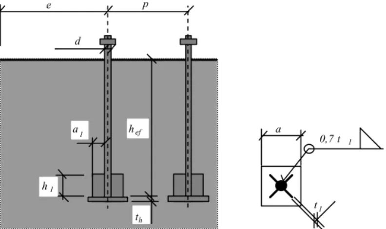
where the geometry conditions, see Figure 2.1.1, are introduced by
a a a a a h b r 1 1 2 5 5 = + +
m i n , a1≥a (2.1.2)
b b b b b h a r 1 1 2 5 5 = + +
m i n , b1 ≥b (2.1.3)
follows
f =
k f
j
j ck
β γ
j c
(2.1.4)
where joint coefficient is taken under typical conditions with grout as βj = 2 / 3. This factor βj represents the fact that the resistance under the plate might be lower due to the quality of
the grout layer after filling.
a
h
a a
b b
b 1
r
1 r t
FRd
Figure 2.1.1 Evaluation of the concrete block bearing resistance
The flexible base plate, of the area Ap can be replaced by an equivalent rigid plate with area
Aeq, see Fig 2.1.2. The formula for calculation of the effective bearing area under the flexible base plate around the column cross section can be based on estimation of the effective width
c. The prediction of this width c can be based on the T-stub model. The calculation secures that the yield strength of base plate is not exceeded. Elastic bending moment resistance of the base plate per unit length should be taken as
M′= t fy
1 6
2
(2.1.4)
and the bending moment per unit length on the base plate acting as a cantilever of span c is, see Figure 2.1.3.
M′ =1 fj c
2
2
Aeq
Ap
A
c c
c c
Figure 2.1.2 Flexible base plate modelled as a rigid plate of effective area with effective width c
When these moments are equal, the bending moment resistance is reached and the formula evaluating c can be obtained
1 2
1 6
2 2
fj c = t fy (2.1.4)
as
c = t
f 3 f
y j γM0
(2.1.5)
The component is loaded by normal force FSd. The strength, expecting the constant distribution of the bearing stresses under the effective area, see Figure2.1.3 is possible to evaluate for a component by
Fsd ≤ FRd = Ae q f j =(2 c +tw ) L f j (2.1.6)
c
fj
L column
base plate F
t
c tw
Sd FRd
Figure 2.1.3 The T stub in compression, the effective width calculation
The improvement of effective area due to the plate behaviour for plates fixed on three or four edges can be based on elastic resistance of plates (Wald, 1995) or more conservatively can be limited by the deformations of plate as is reached for cantilever prediction. This improvement is not significant for open cross sections, till about 3%. For tubular columns the plate
behaviour increase the strength up to 10% according to the geometry.
The practical conservative estimation of the concentration factor, see Eq. (2.1.1), can be precised by introduction of the effective area into the calculation; into the procedure Eq. (2.1.1) - (2.1.3). This leads however to an iterative procedure and is not recommended for practical purposes.
The grout quality and thickness is introduced by the joint coefficient βj, see SBR (1973). For
βj = 2 / 3, it is expected the grout characteristic strength is not less than 0,2 times the
characteristic strength of the concrete foundation fc.g≥ 0,2 fc and than the thickness of the grout is not greater than 0,2 times the smaller dimension of the base plate tg ≤ 0,2 min (a ; b).
In cases of different quality or high thickness of the grout tg ≥ 0,2 min (a ; b), it is necessary to check the grout separately. The bearing distribution under 45° can be expected in these cases, see Figure 2.1.4., (Bijlaard, 1982).
The influence of packing under the steel plate can be neglected for the design (Wald at al, 1993). The influence of the washer under plate used for erection can be also neglected for design in case of good grout quality fc.g ≥ 0,2 fc. In case of poor grout quality fc.g ≤ 0,2 fc it is necessary to take into account the anchor bolts and base plate resistance in compression separately.
h
t tg
g
t
45o
tg
washer under
packing base plate
tg
o
45
Figure 2.1.4 The stress distribution in the grout
2.1.3.2 Stiffness
The elastic stiffness behaviour of the T-stub components concrete in compression and plate in bending exhibit the interaction between the concrete and the base plate as demonstrated for the strength behaviour. The initial stiffness can be calculated from the vertical elastic deformation of the component. The complex problem of deformation is influenced by the flexibility of the base plate, and by the concrete block quality and size.
The simplified prediction of deformations of a rigid plate supported by an elastic half space is considered first including the shape of the rectangular plate. In a second step, an indication is given how to replace a flexible plate by an equivalent rigid plate. In the last step, assumptions are made about the effect of the size of the block to the deformations under the plate for practical base plates.
The deformation of a rectangular rigid plate in equivalent half space solved by different authors is given in simplified form by Lambe & Whitman, 1967 as
δr α
r
c r
F a
E A
= , (2.1.6)
where
δr is the deformation under a rigid plate,
F the applied compressed force,
ar the width of the rigid plate,
Ec the Young's modulus of concrete,
Ar the area of the plate, Ar = ar L , L the length of the plate,
α a factor dependent on ratio between L and ar .
The value of factor α depends on the Poison's ratio of the compressed material, see in Table 2.1.1, for concrete (ν≈ 0,15). The approximation of this values as α≈0,85 L / ar
can be read from the following Table 2.1.1.
Table 2.1.1 Factor α and its approximation
L / ar α
according to (Lambe and Whitman, 1967)
Approximation as α ≈0 85, L / ar
1 0,90 0,85 1,5 1,10 1,04
2 1,25 1,20 3 1,47 1,47 5 1,76 1,90 10 2,17 2,69
With the approximation for α, the formula for the displacement under the plate can be rewritten
δr
c r
F
E L a
= 0 8 5, (2.1.7)
A flexible plate can be expressed in terms of equivalent rigid plate based on the same deformations. For this purpose, half of a T-stub flange in compression is modelled as shown in Figure 2.1.5.
δ E Ip
x cfl
Figure 2.1.5 A flange of a flexible T-stub
The flange of a unit width is elastically supported by independent springs. The deformation of the plate is a sine function, which can be expressed as
δ (x) = δ sin ( ½ π x / cfl) (2.1.8)
The uniform stress on the plate can then be replaced by the fourth differentiate of the deformation multiplied by E Ip, where E is the Young's modulus of steel and Ip is the moment
of inertia per unit length of the steel plate with thickness t (Ip = t3 / 12).
σ(x) = Es Ip ( ½ π / cfl ) 4
δ sin (½ π x / cfl ) = Es
t3
1 2 ( ½ π / cfl )
4
δ sin ( ½ π x / cfl ) (2.1.9)
The concrete part should be compatible with this stress
δ(x) = σ(x)hef / Ec (2.1.10)
where hef is the equivalent concrete height of the portion under the steel plate. Assume that
hef = ξ cfl hence
δ(x) = σ(x)ξcfl / Ec (2.1.11)
Substitution gives
δ sin (½ πx / cfl ) = E t3 / 12 (½ π / cfl )4 δ sin ( ½ πx / cfl ) ξcfl / Ec (2.1.12)
c = t fl 3
(π )
ξ
2 1 2
4
E
Ec
(2.1.13)
The flexible length cfl may be replaced by an equivalent rigid length cr such that uniform
deformations under an equivalent rigid plate give the same force as the non uniform deformation under the flexible plate:
cr = cfl 2 / π (2.1.14)
The factor ξ represents the ratio between hef and cfl. The value of hef can be expressed as αar.
From Tab. 2.1 can be read that factor α for practical T-stubs is about equal to 1,4. The width
ar is equal to tw + 2 cr, where tw is equal to the web thickness of the T-stub. As a practical
assumption it is now assumed that tw equals to 0,5 cr which leads to
hef = 1,4 ⋅ (0,5 + 2) cr = 1,4 ⋅ 2,5 cfl 2 / π = 2,2 cfl (2.1.15)
hence ξ = 2,2
For practical joints can be estimated by Ec≅ 30 000 N / mm2 and E ≅ 210 000 N / mm2, which
leads to
c = t fl 3 t 3
( ) ( )
, ,
π
ξ π
2 12
2
12 2 2
2 1 0 0 0 0
30 0 0 0 1 98
4 4
E
Ec ≈ ≅ . (2.1.16)
or
cr = 1,26 t ≈ 1,25 t , (2.1.17)
which gives for the effective width calculated based on elastic deformation
aeq.e l = t + 2 , 5 t w (2.1.18)
The influence of the finite block size compared to the infinite half space can be neglected in practical cases. For example the equivalent width ar of the equivalent rigid plate is about tw +
2 cr. In case tw is 0,5 cr and cr = 1,25t the width is ar = 3,1 t. That means, peak stresses are
even in the elastic stage spread over a very small area.
In general, a concrete block has dimensions at least equal to the column with and column depth. Furthermore it is not unusual that the block height is at least half of the column depth. It means, that stresses under the flange of a T-stub, which represents for instance a plate under a column flange, are spread over a relative big area compared to ar = 3,1 t. If stresses are
spread, the strains will be low where stresses are low and therefore these strains will not contribute significantly to the deformations of the concrete just under the plate. Therefore, for
simplicity it is proposed to make no compensation for the fact that the concrete block is not infinite.
From the strength procedure the effective with of a T-stub is calculated as
a = t + 2 c = t + 2 t
f 3 f
eq.str w w
y j γM 0
(2.1.19)
Based on test, see Figure 2.1.7 - 2.1.8, and FE simulation, see Figure 2.1.9, it may occur that the value of aeq.str is also a sufficient good approximation for the width of the equivalent rigid
plate as the expression based on elastic deformation only. If this is the case, it has a practical advantage for the application by designers. However, in the model aeq.str will become
dependent on strength properties of steel in concrete, which is not the case in the elastic stage, On Figure 2.1.6 is shown the influence of the base plate steel quality for particular example on the concrete quality - deformation diagram for flexible plate t = tw = 20 mm, Leff = 300 mm, F = 1000 kN. From the diagram it can be seen that the difference between
aeq.el = tw + 2,5 t and aeq.str = tw + 2 c is limited.
S 235, S 275, S 355 for strength, S 235 for strength, S 275 for strength, S 355
elastic model,
Concrete, f , MPa
ck
aeq.str
eq.el
a
0,00 0,05 0,10 0,15 0,20 0,25
10 15 20 25 30 35 40
Deformation, mm
L = 300 mm
t = 20 mmw
F = 1000 kN
δ
t = 20 mm
Figure 2.1.6 Comparison of the prediction of the effective width on concrete - deformation diagram for particular example for unlimited concrete block kj = 5, base plate and web
thickness 20 mm, L = 300 mm, force F = 1000 kN
The concrete surface quality is affecting the stiffness of this component. Based on the tests Alma and Bijlaard, (1980), Sokol and Wald, (1997). The reduction of modulus of elasticity
of the upper layer of concrete of thickness of 30 mm was proposed (Sokol and Wald, 1997) according to the observation of experiments with concrete surface only, with poor grout quality and with high grout quality. For analytical prediction the reduction factor of the surface quality was observed from 1,0 till 1,55. For the proposed model the value 1,50 had been proposed, see Figure 2.1.12 and 2.1.13, see Eq. (2.1.20).
The simplified procedure to calculate the stiffness of the component concrete in compression and base plate in bending can be summarised in Eurocode 3 Annex J form as
E 275 , 1
L a E E 85 , 0 * 5 , 1
L a E E F
kc = = c eq.el = c eq.el
δ , (2.1.20)
where
aeq.el the equivalent width of the T-stub, ae.el = tw + 2,5 t,
L the length of the T-stub,
t the flange thickness of the T-stub, the base plate thickness,
tw the web thickness of the T-stub, the column web or flange thickness.
2.1.4 Validation
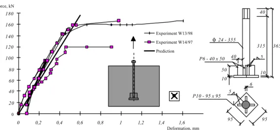
The proposed model is validated against the tests for strength and for stiffness separately. 50 tests in total were examined in this part of study to check the concrete bearing resistance (DEWOLF, 1978, HAWKINS, 1968). The test specimens consist of a concrete cube of size from 150 to 330 mm with centric load acting through a steel plate. The size of the concrete block, the size and thickness of the steel plate and the concrete strength are the main variables.
t / e f / f
0 1 2
0 5 10 15 20 25 30
Anal.
Exp. e
j cd
Figure 2.1.7 Relative bearing resistance-base plate slenderness relationship (experiments DeWolf, 1978, and Hawkins, 1968)
Figure 2.1.7 shows the relationship between the slenderness of the base plate, expressed as a ratio of the base plate thickness to the edge distance and the relative bearing resistance. The design approach given in Eurocode 3 is in agreement with the test results, but conservative. The bearing capacity of test specimens at concrete failure is in the range from 1,4 to 2,5 times the capacity calculated according to Eurocode 3 with an average value of 1,75.
0 20 40 60
700 600 500 400 300 200 100 0
10 30 50
a
bc
d e f
<>
<> <>
f , MPa N, kN
cd
Anal. a b c d e f
Exp. <> 0,76 mm
1,52 mm 3,05 mm 6,35 mm 8,89 mm 25,4 mm
t =
a x b = 600 x 600 mm
The influence of the concrete strength is shown on Figure 2.1.8, where is shown the validation of the proposal based on proposal tw + 2 c. A set of 16 tests with similar geometry and
material properties was used in this diagram from the set of tests (Hawkins, 1968). The only variable was the concrete strength of 19, 31 and 42 MPa.
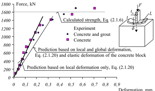
0 200 400 600 800 1000 1200 1400 1600 1800
0 0,1 0,2 0,3 0,4 0,5 0,6 0,7 0,8 0,9
Deformation, mm Force, kN
Concrete and grout Concrete
Experiment
Prediction based on local and global deformation,
Prediction based on local deformation only, Eq. (2.1.20) Calculated strength, Eq. (2.1.6)
Eq. (2.1.20) and elastic deformation of the concrete block L F
δ t
t w
Figure 2.1.9 Comparison of the stiffness prediction to Test 2.1, (Alma and Bijlaard, 1980), concrete block 800x400x320 mm, plate thickness t = 32,2 mm, T stub length L = 300 mm
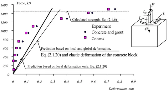
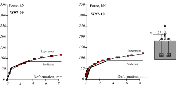
The stiffness prediction is compared to tests Alma and Bijlaard, (1980) in Figure 2.1.9. and 2.1.10. The tests of flexible plates on concrete foundation are very sensitive to boundary conditions (rigid tests frame) and measurements accuracy (very high forces and very small deformations). The predicted value based on eq. (2.1.7) is the local deformation only. The elastic global and local deformation of the whole concrete block is shown separately. Considering the spread in test results and the accuracy achievable in practice, the comparison shows a sufficiently good accuracy of prediction.
0 200 400 600 800 1000 1200 1400 1600
0 0,1 0,2 0,3 0,4 0,5 0,6 0,7 0,8 0,9 Deformation, mm
Force, kN
Concrete and grout Concrete
Experiment
Prediction based on local deformation only, Eq. (2.1.20) Calculated strength, Eq. (2.1.6)
Prediction based on local and global deformation,
Eq. (2.1.20) and elastic deformation of the concrete block
L F
δ t
t w
Figure 2.1.10 Comparison of the stiffness prediction to Test 2.2, (Alma and Bijlaard, 1980), concrete block 800x400x320 mm, plate thickness t = 19 mm, T stub length L = 300 mm
Deformation, mm
Force, kN Prediction, Eq. (2.1.20)
0 100 200 300 400 500 600
0 0,1 0,2 0,3 0,4 0,5 0,6
Experiment Excluding concrete surface quality factor
W97-15
Parallel line to prediction
L F
δ
t t w
Figure 2.1.11 Comparison of the stiffness prediction to Test W97-15, repeated loading, cleaned concrete surface without grout only (Sokol and Wald, 1997), concrete block
Deformation, mm Force, kN
0 100 200 300 400 500 600
0 0,5 1 1,5 2 2,5
Experiment W97-21
Parallel lines
L F
d
t t w
to prediction Prediction, Eq. (2.1.20)
Excluding concrete surface quality factor
Figure 2.1.12 Comparison of the stiffness prediction to Test W97-15 repeated and increasing loading, cleaned concrete surface low quality grout (Sokol and Wald, 1997), concrete block
550 x 550 x 500 mm, plate thickness t = 12 mm, T stub length L = 335 mm
The comparison of local and global deformations can be shown on Finite Element (FE) simulation. In Figure 2.1.11 the prediction of elastic deformation of rigid plate 100 x 100 mm on concrete block 500 x 500 x 500 mm is compared to calculation using the FE model.
0,1
Vertical deformation along the block height
foot of the concrete block top of the concrete block Vertical deformation at the surface, mm
elastic deformation of the whole block
predicted value eq. (2.1.20)
0,1 0
deformation at the axis elastic deformation
deformation at the edge
Vertical deformation, mm
0,0
edge axis
}
local deformation under plateF
δglob δedge
δaxis
Figure 2.1.13 Calculated vertical deformations of a concrete block 0,5 x 0,5 x 0,5 m loaded to a deflection of 0,01 mm under a rigid plate 0,1 x 0,1 m; in the figure on the right, the
deformations along the vertical axis of symmetry δaxis are given and the calculated
deformations at the edge δedge, included are the global elastic deformations according to
δglob = F h /(Ec Ac), where Ac is full the area of the concrete block
Based on these comparisons, the recommendation is given that for practical design, besides the local effect of deformation under a flexible plate, the global deformation of the supporting concrete structure must be taken into consideration.
2.2 Column flange and web in compression
2.2.1 Description of the component
In this section, the mechanical characteristics of the “column flange and web in compression” component are presented and discussed. This component, as its name clearly indicates, is subjected to tension forces resulting from the applies bending moment and axial force in the column (Figure 2.2.1).
The proposed rules for resistance and stiffness evaluation given hereunder are similar to those included in revised Annex J of Eurocode 3 for the “beam flange and web in compression” component in beam-to-column joints and beam splices.
Figure 2.2.1 Component “column flange and web in compression”
2.2.2 Resistance
When a bending moment M and a axial force N are carried over from the column to the concrete block, a compression zone develops in the column, close to the column base; it includes the column flange and a part of the column web in compression. The compressive force Fc carried over by the joint may, as indicated in Figure 2.2.2, is quite higher than the compressive force F in the column flange resulting from the resolution, at some distance of the joint, of the same bending moment M and axial force N. In Figure 2.2.2, the forces F and
Fc are applied to the centroï d of the column flange in compression.
This assumption is usually made for sake of simplicity but does not correspond to the reality as the compression zone is not only limited to the column flange.
The force Fc, quite localized, may lead to the instability of the compressive zone of the column cross-section and has therefore to be limited to a design value which is here defined in a similar way than in Annex J for beam flange and web in compression :
) /(
. .
.fbRd cRd c fc
c M h t
F = − (2.2.1)
where :
Mc.Rd is the design moment resistance of the column cross-section reduced, when necessary, by the shear forces; Mc.Rd takes into consideration by itself the potential risk of instability in the column flange or web in compression;
hb is the whole depth of the column cross-section;
tfb is the thickness of the column flange.
• M and N applied as in Figure 2.2.1
• F = N/2 + M/(hb-tfb) • Fc = N/2 + M/z
⇒ F < Fc
Figure 2.2.2 Localized compressive force in the column cross-section located close to the column base
It has to be pointed out that Formula (2.2.1) limits the maximum force which can be carried over in the compressive zone of the joint because of the risk of loss of resistance or instability in the possibly overloaded compressive zone of the column located close to the joint. It therefore does not replace at all the classical verification of the resistance of the column
cross-z Fc
F hc - tfc
section.
It has also to be noted that formula (2.2.1) applies whatever is the type of connection and the type of loading acting on the column base. It is also referred to in the preliminary draft of Eurocode 4 Annex J in the case of composite construction and applies also to beam-to-column joints and beam splices where the beams are subjected to combined moments and shear and axial compressive or tensile forces. It is therefore naturally extended here to column bases.
The design resistance given by Formula (2.2.1) has to be compared to the compressive force
Fc (see Figure 2.2.2) which results from the distribution of internal forces in the joint and which is also assumed to be applied at the centroï d of the column flange in compression. It integrates the resistance of the column flange and of a part of the column web; it also covers the potential risk of local plate instability in both flange and web.
2.2.3 Stiffness
The deformation of the column flange and web in compression is assumed not to contribute to the joint flexibility. No stiffness coefficient is therefore needed.
2.3 Base plate in bending and anchor bolt in tension
When the anchor bolts are activated in tension, the base plate is subjected to tensile forces and deforms in bending while the anchor bolts elongate. The failure of the tensile zone may result from the yielding of the plate, from the failure of the anchor bolts, or from a combination of both phenomena.
Two main approaches respectively termed "plate model" and "T-stub model" are referred to in the literature for the evaluation of the resistance of such plated components subjected to transverse bolt forces.
The first one, the "plate model", considers the component as it is - i.e. as a plate - and formulae for resistance evaluation are derived accordingly. The actual geometry of the component, which varies from one component to another, has to be taken into consideration in an appropriate way; this leads to the following conclusions :
• the formulae for resistance varies from one plate component to another;
• the complexity of the plate theories are such that the formulae are rather complicated and therefore not suitable for practical applications.
The T-stub idealisation, on the other hand, consists of substituting to the tensile part of the joint T-stub sections of appropriate effective length leff, connected by their flange onto a presumably infinitely rigid foundation and subject to a uniformly distributed force acting in the web plate, see Figure 2.3.1.
eff
web
flange
F
t e m
l
Figure 2.3.1 T-stub on rigid foundation
In comparison with the plate approach, the T-stub one is easy to use and allows to cover all the plated components with the same set of formulae. Furthermore, the T-stub concept may also be referred to for stiffness calculations as shown in (Jaspart, 1991) and Yee, Melchers, 1986).
This explains why the T-stub concept appears now as the standard approach for plated components and is followed in all the modern characterisation procedures for components, and in particular in Eurocode 3 revised Annex J (1998) for beam-to-column joints and column bases. In the next pages, the evaluation of the resistance and stiffness properties of the T-stub are discussed in the particular context of column bases and proposals for inclusion in forthcoming European regulations are made.
2.3.1 Design resistance of plated components
2.3.1.1 Basic formulae of Eurocode 3
The T-stub approach for resistance, as it is described in Eurocode 3, has been first introduced by Zoetemeijer (1974) for unstiffened column flanges. It has been then improved (Zoetemeijer, 1985) so as to cover other plate configurations such as stiffened column flanges and end-plates. In Jaspart (1991), it is also shown how to apply the concept to flange cleats in bending.
In plated components, three different failure modes may be identified :
a) Bolt fracture without prying forces, as a result of a very large stiffness of the plate (Mode 3) b) Onset of a yield lines mechanism in the plate before the strength of the bolts is exhausted
(Mode 1)
c) Mixed failure involving yield lines - but not a full plastic mechanism - in the plate and exhaustion of the bolt strength (Mode 2).
Similar failure modes may be observed in the actual plated components (column flange, end plates, …) and in the flange of the corresponding idealised T-stub. As soon as the effective length leff of the idealised T-stubs is chosen such that the failure modes and loads of the actual
plate and the T-stub flange are similar, the T-stub calculation can therefore be substituted to that of the actual plate.
In Eurocode 3, the design resistance of a T-stub flange of effective length leff is derived as follows for each failure mode :
Mode 3: bolt fracture (Figure 2.3.2.a)
FRd,3= ΣBt Rd. (2.3.1)
Mode 1: plastic mechanism (Figure 2.3.2.b)
F m
m
Rd
eff pl Rd ,
,
1 4
= l (2.3.2)
Mode 2: mixed failure (Figure 2.3.2.c)
F m B n
m n
Rd
eff pl Rd t Rd ,
, .
2 2
F
B
Rd.3
t.Rd Bt.Rd
F B
Rd.1
B
Q Q
e
n m
Q Q
Bt.Rd
Bt.Rd
FRd.2
Mode 3 Mode 1 Mode 2
Figure 2.3.2 Failure modes in a T-stub
In these expressions :
mpl,Rd is the plastic moment of the T-stub flange per unit length ( y M0 2
/ f t 4
1
γ ) with t = flange thickness, fy = yield stress of the flange, γM0 = partial safety
factor)
m and e are geometrical characteristics defined in Figure 2.3.2.
Σ Bt.Rd is the sum of the design resistances Bt.Rd of the bolts connecting the T-stub to the foundation (Bt.Rd = 0,9 As fub / γMb where As is the tensile stress area of
the bolts, fub the ultimate stress of the bolts and γMb a partial safety factor) n designates the place where the prying force Q is assumed to be applied, as
shown in Figure 2.3.2 (n = e, but its value is limited to 1,25 m).
leff is derived at the smallest value of the effective lengths corresponding to all
the possible yield lines mechanisms in the specific T-stub flange being considered.
The design strength FRd of the T-stub is derived as the smallest value got from expressions (2.3.1) to (2.3.3) :
FRd = min(FRd,1,FRd,2,FRd,3) (2.3.4)
In Jaspart (1991), the non-significative influence of the possible shear-axial-bending stress interactions in the yield lines on the design capacity of T-stub flanges has been shown.
In Annex J, the influence on Mode 1 failure of backing plates aimed at strengthening the column flanges in beam-to-column bolted joints is also considered. A similar influence may result, in
column bases, from the use of washer plates. The effect of the latter on the base plate resistance will be taken into consideration in a similar way than it is done in Annex J for backing plates.
This calculation procedure recommended first by Zoetemeijer has been refined when revising the Annex J of Eurocode 3.
Eurocode 3 distinguishes now between so-called circular and non-circular yield lines mechanisms in T-stub flanges (see Figure 2.3.3.a). These differ by their shape and lead to specific values of T-stub effective lengths noted respectively leff,cp and leff,np. But the main difference between circular and non-circular patterns is linked to the development or not of prying forces between the T-stub flange and the rigid foundation : circular patterns form without any development of prying forces Q, and the reverse happens for non-circular ones.
The direct impact on the different possible failure modes is as follows :
Mode 1 : the presence or not of prying forces do not alter the failure mode which is linked in both cases to the development of a complete yield mechanism in the plate. Formula (2.3.2) applies therefore to circular and non-circular yield patterns.
Mode 2 : the bolt fracture clearly results here from the over-loading of the bolts in tension because of prying effects; therefore Mode 2 only occurs in the case of non-circular yield lines patterns.
Mode 3 : this mode does not involve any yielding in the flange and applies therefore to any T-stub.
As a conclusion, the calculation procedure differs according to the yield line mechanisms developing in the T-stub flange (Figure 2.3.3.b) :
FRd =min(FRd,1;FRd,3) for circular patterns (2.3.5.a)
FRd =min(FRd,1;FRd,2;FRd,3) for non-circular patterns (2.3.5.b)
In Annex J, the procedure is expressed in a more general way. All the possible yield line patterns are considered through recommended values of effective lengths grouped into two categories : circular and non-circular ones. The minimum values of the effective lengths - respectively termed leff,cp and leff,np - are therefore selected for category. The failure load is
then derived, by means of Formula (2.3.4), by considering successively all the three possible failure modes, but with specific values of the effective length :
Mode 1 : leff,1 =min(leff,cp;leff,nc) (2.3.6.a)
Mode 2 : leff,2=leff nc, (2.3.6.b)
Mode 3 : - (2.3.6.c)
Circular pattern (leff,cp) Non-circular patterns (leff,nc) (a) Different yield line patterns
0 0,2 0,4 0,6 0,8 1
0 0,5 1 1,5 2 2,5
Mode 1
Mode 2
Mode 3
Mode 1*
F/ Σ Bt.Rd
4 leff Mpl.Rd / Σ Bt.Rd
(b) Design resistance
Figure 2.3.3 T-stub resistance according revised Annex J
2.3.1.2 Alternative approach for Mode 1 failure
The accuracy of the T-stub approach is quite good when the resistance is governed by failure modes 2 and 3. The formulae for failure mode 1, on the other hand, has been seen quite conservative, and sometimes too conservative, when a plastic mechanism forms in the T-stub flange (Jaspart, 1991).
Therefore the question raised whether refinements could be brought to the T-stub model of Eurocode 3 with the result that the amended model would provide a higher resistance for failure mode 1 without altering significantly the accuracy rega rding both failure modes 2 and 3.
In (Jaspart, 1991), an attempt has been made in this respect. In the Zoetemeijer’s approach, the forces in the bolts are idealised as point loads. Thus, it is never explicitly accounted for the actual sizes of the bolts and washers. If this is done, the following resistance may be expressed for Mode 1 (Jaspart, 1991):
[
]
F n e m
mn e m n
Rd
w eff pl Rd w
,
, ,
( )
( )
1
1
8 2
2
= −
− +
l
(2.3.7)
with ew = 0.25 dw (dw designates the diameter of the bolt/screw or of the washer if any.
Of course, Equation (2.3.7) confines itself to Zoetemeijer's formulae (2.3.2) when distance ew is vanishing.
During the recent revision of Annex J of Eurocode 3, formula (2.3.7) which describes the Mode 1 failure as dependent on the actual bolt dimensions has been agreed for inclusion as an alternative to formula (2.3.2).
2.3.2 Initial stiffness of plated components
2.3.2.1 Application of the T-stub approach
For plated components, it is also referred to the T-stub concept, see Figure 2.3.4.
Figure 2.3.4 T-stub elastic deformability
In a T-stub, the tensile stiffness results from the elastic deformation of the T-stub flange in bending and of the bolts in tension (the role of the latter is plaid by the anchor bolts in section 2.3.3 dealing explicitly with column bases). When evaluating the stiffness of the T-stub, the compatibility between the respective deformabilities of the T-stub flange and of the bolts has to be ensured :
b p =∆
∆*
(2.3.8)
where ∆p* is the deformation of the end-plate at the level of the bolts; ∆b is the elongation of the bolts.
In Jaspart (1991), expressions providing the elastic initial stiffness of the T-stub are proposed; they allow the coupling effect between the T-stubs to be taken into consideration. These expressions slightly differ from those given in the original publication of Yee and Melchers (1986).
The elongation ∆b of the bolts simply results from the elongation of the bolt shank subjected to
tension:
F B
Q
∆p*
0,75n m 4/5 2 a
a
F B B
Q Q
0,75n m
b S
b L
A E
B
=
∆ (2.3.9)
where Lbis approximately defined as the length of the bolt shank in Eurocode 3. From these considerations, the elastic deformation of the two T-stub may be derived :
p , i p
k E
F
=
∆ (2.3.10)
where the stiffness coefficient ki,p is expressed as :
1 p
,
i q )
4 1 8 1 ( Z k
−
−
= α (2.3.11)
S b p
A Z
a Z q
2
2 1
l
+ =
α
(2.3.12)
In these formulae :
3 3 /bt
2
Z = l l =2(m +0,75n )
3 1 1,5α 2α
α = − b is the T-stub length
3 2 2 6α 8α
α = − α =0,75 n / l
All the geometrical properties are defined in Figure 3.2.4.
The validity of these formulae has been demonstrated in Jaspart (1991) on the basis of a quite large number of comparisons with test results on joints with end-plate and flange cleated connections got from the international literature.
2.3.2.2 Simplified stiffness coefficients for inclusion in Eurocode 3
The application of the T-stub concept to a simplified stiffness calculation - as that to be included in a code such Eurocode 3 - requires to express the equivalence between the actual component and the equivalent T-stub in the elastic range of behaviour and that, in a different way than at collapse; this is achieved through the definition of a new effective length called
view of the determination of the stiffness coefficient kip, two problems have to be
investigated:
• the response of a T-stub in the elastic range of behaviour;
• the determination of leff ini, .
These two points are successively addressed hereunder. T-stub response
The T-stub response in the elastic range of behaviour is covered in section 2.3.1.1. The corresponding expressions are rather long to apply, but some simplifications may be introduced:
• to simplify the formulae: n is considered as equal to 1,25 m;
• to dissociate the bolt deformability (Figure 2.3.5.c) from that of the T-sub (Figure 2.3.5.b). The value of q given by expressions (2.3.12) may then be simplified to :
3 2
3
2 1
8 6
2 5 , 1 q
α α
α α α
α
− − =
= (2.3.13)
as soon as it is assumed, as in Figure 2.3.5.b, that the bolts are no more deforming in tension
(As= ∞). q further simplifies to:
282 , 1
q = (2.3.14)
by substituting 1,25 m to 0,75 n as assumed previously.
The stiffness coefficient given by formula (2.3.11) therefore becomes :
3 ini , eff 3 p
, i
) m 5 , 4 ( 2
t 64 , 193 Z
64 , 193
k = = l (2.3.15)
Figure 2.3.5 Elastic deformation of the T-stub Finally : 3 3 ini , eff 3 3 ini , eff p , i m t m t 063 , 1
k = l ≈l (2.3.16)
In the frame of the assumptions made, it may be shown that the prying effect increases the bolt force from 0,5 F to 0,63 F (Figure 2.3.5.c). In Eurocode 3, the deformation of a bolt in tension is taken as equal to :
s b b A E L B =
∆ (2.3.17)
By substituting B by 0,63 F in (2.3.17), the stiffness coefficient of a bolt row with two bolts may be derived :
b s b , i L A 6 , 1
k = (2.3.18)
Definition of effective length lleff,ini
In Figure 2.3.5.c, the maximum bending moment in the T-stub flange (points A) is expressed as Mmax = 0,322 F m. Based on this expression, the maximum elastic load (first plastic hinges in the T-stub at points A) to be applied to the T-stub may be derived :
0 M y 2 ini , eff 0 M y 2 ini , eff e f m 288 , 1 t 4 f t m 288 , 1 4 F γ γ l l
In Annex J, the ratio between the design resistance and the maximum elastic resistance of each of the components is taken as equal to 3/2 so :
MO y 2 ini , eff e Rd
f m 859 , 0
t F
2 3 F
γ
l
l =
= (2.3.20)
As, in Figure 2.3.5.b, the T-stub flange is supported at the bolt level, the only possible failure mode of the T-stub is the development of a plastic mechanism in the flange. The associated failure load is given by Annex J as:
Mo y 2 eff Rd Rd
m f t F
F
γ
l
=
= (2.3.21)
where leff is the effective length of the T-stub for strength calculation. By identification of expressions (2.3.20) and (2.3.21), leff ini, may be derived :
eff eff
ini ,
eff 0,859 l 0,85 l
l = = (2.3.22)
Finally, by introducing equation (2.3.22) in the expression (2.3.18) giving the value of ki,p for any plated component :
3 3 1 , eff p
, i
m t 85 , 0
k = l (2.3.23)
2.3.3 Extension to base plates
To evaluate the resistance and stiffness properties of a base plate in bending and anchor bolts in tension, reference is also made to the T-stub idealisation.
2.3.3.1 Resistance properties
Three failure modes are identified in Section 2.3.1.1 for equivalent T-stubs of beam end-plates and column flanges: Mode 1, Mode 2 and Mode 3. Related formulae may be applied to column base plates as well.
in tension is such, in comparison to the flexural deformability of the base plate, that no prying forces develop at the extremities of the T-stub flange. In this case, the failure results either from that of the anchor bolts in tension (Mode 3) or from the yielding of the plate in bending (see Figure 2.3.6) where a “two hinges” mechanism develops in the T-stub flange. This failure is not likely to appear in beam-to-column joints and splices because of the limited elongation of the bolts in tension. This particular failure mode is named “Mode 1*”.
F*
B B
Rd.1
Figure 2.3.6 Mode 1** failure
The corresponding resistance writes :
m m 2
FRd**.1 = leff pl.Rd (2.3.24)
When the Mode 1* mechanism forms, large base plate deformations develop; they may result in contacts between the concrete block and the extremities of the T-stub flange, i.e. in prying forces. Further loads may therefore be applied to the T-stub until failure is obtained through Mode 1 or Mode 2. But to reach this level of resistance, large deformations of the T-stub are necessary, what is not acceptable in design conditions. The extra-strength which separates Mode 1* from Mode 1 or Mode 2 in this case is therefore disregarded and Formula (2.3.24) is applied despite the discrepancy which could result from comparisons with some experimental tests.
As a result, in cases where no prying forces develop, the design resistance of the T-stub is taken as equal to :
(
Rd,3)
** 1 , Rd
Rd min F ,F
F = (2.3.25)
when FRd,3 is given by formula (2.3.1).
In other cases, the common procedure explained in section 2.3.1 is followed.
The criterion to distinguish between situations with and without prying forces is discussed in section 2.3.3.3.
differentiated when deriving the effective length leff of the T-stub :
• The non-circular patterns referred to in revised Annex J of Eurocode 3 cover cases where prying forces develop at the extremities of the plated component.
• The circular patterns develop without any prying.
Concerning Mode 1* failure, only circular patterns have therefore to be taken into consideration and the non-circular patterns proposed by Eurocode3 have to be disregarded. Mode 1* identifies then exactly to Mode 1 and, in order to ensure that the design resistances provided by formulae (2.3.2) and (2.3.24) are equal, the effective lengths for circular patterns defined in revised Annex J have to be multiplied by a factor 2 before being implemented in Formula (2.3.24).
Besides that, non-circular patterns not involving prying forces in the bolts may occur. These ones may be considered through Formula (2.3.24), but by introducing appropriate effective length characteristics. The lowest of the effective lengths between those derived for circular and non-circular patterns respectively is that which will determines the design resistance of the T-stub.
Table 2.3.1 indicates how to select the values of leff for two classical base plate configurations, in cases where prying forces develop and do not develop.
2.3
1
PRYING FORCES DEVELOP
PRYING FORCES DO NOT DEVELOP
Figure 2.3.7
Anchor bolts
lo
c
ated between the flanges
()
()
2 1 1, eff 2 1 ; min m 2 e 25, 1 m 4 m 2 l l l l l = = + − = π α lleff, 2 1 = where m and nare represented in Figure 2.3.7. and
α
is defined in EC3 Annex J.
()
()
2 1 1, eff 2 1 ; min m 4 e 25, 1 m 4 m 2 l l l l l = = + − = π α lleff, 2 1 = where m and nare represented in Fi
gure 2.3.7. and
α
is defined in EC3 Annex J.
Figure 2.3.8 Anchor bolts base plate l1 = 4.m x+1,25 e x l2 = 2 π mx l3 = 0,5.b p l4 = 0,5.w+2.m x+0,625.e x l5 = e+2.m x+0,625.e x l6 = e 2 mx + π
()
6 5 4 3 2 1 1, eff ; ; ; ; ; min l l l l l l l =()
5 4 3 1 2, eff ; ; ; min l l l l l = where bp, m, e, m
x, e
x
and
w
are given
in Figure 2.3.8.
l1 = 4.m x+1,25 e x l2 = 4 π mx l3 = 0,5.b p l4 = 0,5.w+2.m x+0,625.e x l5 = e+2.m x+0,625.e x l6 = e 4 m 2 x + π
()
6 5 4 3 2 1 1, eff ; ; ; ; ; min l l l l l l l =()
5 4 3 1 2, eff ; ; ; min l l l l l = where bp, m, e, m
x, e
x
and
w
are given
in Figure 2.3.8.
Table
2.3.1
Values of the
T-stub effective length e m bp mx ex e w e
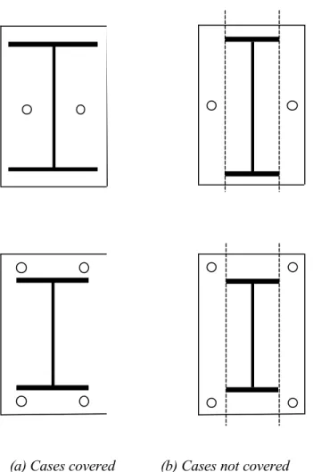
It has to be noted that these formulae only apply to base plates where the anchor bolts are not located outside the beam flanges, as indicated in Figure 2.3.9.
(a) Cases covered (b) Cases not covered
Figure 2.3.9 Limits of validity of the formulae given in Figures 2.3.7 and 2.3.8.
2.3.3.2 Stiffness properties
The elastic deformation of a T-stub in tension is discussed in section 2.3.2.1 and accurate formulae for stiffness evaluation are suggested. They have been used in section 2.3.2.2 to derive simplified expressions for inclusion in Revised Annex J of Eurocode 3.
• the stiffness coefficient for the T-stub flange in bending :
3 3 eff p
m t 85 , 0
• the stiffness coefficient for the anchor bolts in tension:
b s b
L A 6 , 1
k = (2.3.27)
where Lb is the anchor bolt length described hereunder. These two expressions relate to situations where prying forces develop at the extremities of the T-stub flange as a result of a limited bolt-axial deformation in comparison with the bending deformation of the flange.
In "no prying cases", the deformation ∆p of the base plate is easily derived as :
p , i p
k E
F
=
∆ (2.3.28.a)
where the stiffness coefficient ki,p is expressed as :
3 3 ini , eff p , i
m 2
t l
k = (2.3.29.b)
and that of the bolts (without preloading) :
b , i b
k E
F
=
∆ (2.3.30.a)
with :
b s b , i
L A 2
k = (2.3.31.b)
Lb is the effective free length of the anchor bolts (Figure 3.2.10). It is defined as the sum of two contributions Lfl and Lel. Lfl is the free length of the anchor bolts, i.e. the part of the bolt which is not embedded. Lel is the equivalent free length of the embedded part of the anchor bolt; it may be approximated to 8d (Wald, 1993), where d is the nominal diameter of the anchor bolt. Should the embedded length of the bolt be shorter than 8d, then the actual length of the bolt would be considered. A justification of this definition of Lel is given in section 2.3.5.
Lfl
L d
el
L
Figure 2.3.10 Effective length of the anchor bolts
If the approximation of the leff,ini value suggested in section 2.3.3.2 is again considered - formula (2.3.26) -, the stiffness coefficient for the base plate in the case of "no prying" conditions may be finally expressed as :
3 3 eff p
, i
m t l 425 , 0
k = (2.3.32)
2.3.3.3 Boundary for prying effects
The elastic deformed shape of a T-stub in tension depends on the relative deformability of the flange in bending and the anchor bolts in tension (see section 2.3.2). In Figure 3.2.11, the bolt and flange deformations compensate such that the contact force Q just vanishes. For a higher bolt deformability, no contact will develop, while contact forces will appear for a lower bolt deformability. The situation illustrated in Figure 2.3.11 therefore constitutes a limit case to which a prying boundary may be associated. This is expressed as follows :
3 eff
s 2 boundary . b
t A n m 7 L
l
= . (2.3.33)
If, as a further assumption, n is defined as equal to 1,25 m (section 2.3.2.2), then :
3 eff
s 3 boundary
. b
t A m 82 , 8 L
l
= . (2.3.34)
n m F
Q = 0
Θp ∆b
∆b = Θp n
Q = 0