Indoor localization using controlled ambient sounds

Indoor localization using controlled ambient sounds

Ish Rishabh

University of California, Irvine Irvine, CA, USA Email: [email protected]

Don Kimber

Palo Alto, CA, USA Email: [email protected]

John Adcock

Palo Alto, CA, USA Email: [email protected]

Abstract—Audio-based receiver localization in indoor environ-ments has multiple applications including indoor navigation, loca-tion tagging, and tracking. Public places like shopping malls and consumer stores often have loudspeakers installed to play music for public entertainment. Similarly, office spaces may have sound conditioning speakers installed to soften other environmental noises. We discuss an approach to leverage this infrastructure to perform audio-based localization of devices requesting local-ization in such environments, by playing barely audible controlled sounds from multiple speakers at known positions. Our approach can be used to localize devices such as smart-phones, tablets and laptops to sub-meter accuracy. The user does not need to carry any specialized hardware. Unlike acoustic approaches which use high-energy ultrasound waves, the use of barely audible (low energy) signals in our approach poses very different challenges. We discuss these challenges, how we addressed those, and experimental results on two prototypical implementations: a request-play-record localizer, and a continuous tracker. We evaluated our approach in a real world meeting room and report promising initial results with localization accuracy within half a meter 94% of the time. The system has been deployed in multiple zones in our office building and is used on a regular basis.

I. INTRODUCTION

Indoor localization has several applications such as indoor navigation, location tagging, and tracking. Due to the obstruc-tion of direct line-of-sight to satellites in indoor environments, Global Positioning System (GPS) does not work well indoors. Researchers have actively explored alternative mechanisms for indoor localization. Many systems have been proposed that utilize different modalities like wi-fi, RFID or camera-networks. These systems often employ equipment which is expensive or deployed solely for the purpose of localization. Many of these systems (like Wi-Fi and RFID-based) fail to achieve a sub-meter accuracy which is often required for applications like indoor navigation. Some systems have the potential to infringe upon user privacy (such as camera-based tracking systems or systems using microphones deployed in the environment).

In developing our approach to indoor navigation, we have focused on several guiding principles. We want accuracy on the order of a meter or better. The setup should not require any dedicated expensive equipment to be installed in the en-vironment. Users of our system should not require specialized gadgets or procedures; an app running on a smartphone should be enough. Moreover, our system should respect user privacy and should not require potentially invasive microphones or cameras to be installed in the environment.

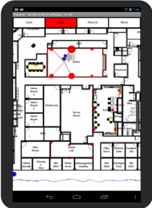
Fig. 1. GUI for the tracking server. The top panel shows cross-correlations (in black) of the recorded signal with 6 reference signals played from speakers, with estimated delays indicated as small green bars. The tall green line indicates the estimated time when the signals were played. The bottom panel depicts a map of the room, showing speaker positions as red circles. The green dot indicates estimated microphone position, and green lines show which 4 speakers out of the 6 were used for the estimate.

Large indoor locations such as malls, consumer stores and museums are usually equipped with loudspeakers for public address, or to play music for customer entertainment. Indoor workspaces often includesound conditioningspeakers to play noise or ambient sounds to soften other environmental noise. With little modification, these systems can be leveraged to provide additional functionality to allow users to determine their location. This work introduces an approach that uses controlled ambient sounds played through multiple speakers, which can be recorded by a smart-device (smart-phone, tablet 978-1-4673-1954-6/12/$31.00 2012 IEEE

or laptop). The recorded audio can then be used to determine a user’s location.

The audio played from each speaker contains a low energy pseudo-random white noise sequence, possibly mixed with music or other sounds for human consumption. The audio is played using any multi-track audio system, such as commonly available 5.1 or 7.1 surround systems, so that the source tracks are known to be synchronized with each other. No synchronization between the source and recording device is required. The recorded audio is analyzed to estimate the arrival times of the signals from each speaker. These estimates are then used to determine both the microphone position, and the synchronization between speakers and microphone. Our con-tributions lie in proposing an audio-based receiver localization system that uses low-energy (barely audible) audio signals for indoor localization. We use windowed cross-correlation of long duration signals to improve signal-to-noise ratio and to account for mismatched speeds between the playback and receiver system clocks, i.e. the clock drift.

To demonstrate our approach, we have developed a system, which provides localization services in three zones of our research center - the main meeting room, the kitchen area, and a lab area. A user interface to the localization system is shown in Figure 1. It may be run as a standalone client on a laptop, or as a server back end, providing estimates to Android clients as shown in Figure 2.

II. RELATEDWORK

Many systems attempt to address the problem of indoor localization using different modalities. Systems using wifi [1], [2] report a median localization error of more than a meter, and typically involve extensive setup and tuning. Localization error for systems based on GSM [3], IR [4] and RFID [5] also fall in similar range. In order to attain sub-meter accuracy, optical and acoustic based systems have to be used.

Localization systems can conceptually be classified into source localization systems andreceiver localization systems. Camera-based (optical) systems [6], [7] and most acoustic sys-tems using microphones [8], [9], [10], [11], [12] try to localize asourceby sensing its signal through multiple receivers with known positions. Such systems can potentially violate user privacy by recording their video or voices without explicit approval. Another undesirable property of audio-based source localization systems is that the device to be localized needs to continuously make audible sounds, which may be a cause of irritation to the user [12].

On the other hand, in receiver localization systems, a receiver senses the ambient signal which is then processed to determine the receiver’s location. The ambient signal can ei-ther beuncontrolledorcontrolled. Systems using uncontrolled signals either employ multipleknownreceivers [13] as part of the system (potentially violating privacy) or use collaborative sensing. Collaborative sensing [14] requires multipleunknown receivers that try to simultaneously localize themselves. Some systems like [15] take a hybrid approach by using both a source and receiver in the client device. Such collaborative

Fig. 2. Android App showing map of building. The App is streaming audio buffers to a processing server, which returns position estimates in real time. Red dots show positions of loudspeakers in three zones covered. The blue pin indicates estimated position, which is updated in real time. The size of the dots in that zone indicate peak strength, and red lines indicate which speakers were used for estimation.

systems cannot be used to localize a single receiver. In other systems like [16] the receiver senses multiple characteristic spatial signatures in an environment to identify which part of the environment it is in. Systems such as [17], [18] model the acoustic background spectrum to produce location dependent signatures. These signature based ‘fingerprinting’ methods have the advantage of not requiring installed infrastructure, but require training, provide only coarse level (e.g. room level) localization, and are subject to sporadic changes in background acoustics.

The proposed system differs from these systems as it is a receiver localization system using controlled audio sig-nals. Many systems employing ultrasonic waves [19], [20], [21], [22], [23], [24] usually have a better ranging accuracy compared to those that use audible sound, but these systems have several limitations. They require dedicated special in-frastructure - ultrasound transducers and wireless coordination networks that are not used for any other purpose [25]. Most low-end and PC speakers have a frequency response limited to 20kHz, and many smartphones microphones are unsuitable for ultrasonic signals. Also, ultrasound has a limited range compared to audible sound due to greater attenuation while propagating through the air. Another difference between

ap-proaches using ultrasound and ours is that ultrasonic systems can afford to use high-energy signals to boost signal-to-noise ratio. We, on the other hand, cannot use high-energy sounds as it might be disturbing to the people in the environment. Hence, our approach is tailored toward localization in low SNR conditions.

We differentiate our work in the following ways. 1) We use low-energy sounds as our reference signals. 2) We improve ‘effective SNR’ in the cross-correlations by

using long duration reference signals and recordings. 3) We assume no explicit prior synchronization between the

speakers and the recording device. This avoids overheads like using a separate RF channel for synchronization. We also introduce the following ideas in this paper. 1) Use of windowed cross-correlation and its modification

to address clock drift (Section IV-C) between playing and recording devices.

2) A simple correlation qualityheuristic to select a subset of speakers so that only those speakers with good cross-correlation peaks are selected for localization. This helps in avoiding speakers for which correlation is very noisy. 3) Use of a solution fitness (residue in Section IV-E) to decide whether the estimated value of t0, to be

introduced later, is accurate. This value of t0 can be

re-used later for better estimation. III. ARCHITECTURE& SYSTEM

We have experimented with several variations of the pro-posed system, and have built a flexible architecture to support different types of experiments and modes of usage. The architecture includes three primary elements: (1) audio players responsible for playing known synchronized tracks from mul-tiple speakers, (2) clients equipped with microphones, running on laptops, tablets or smart phones, and possibly (3) processing servers, which could be used by underpowered clients to perform localization. Depending on usage requirements, audio players may be controllable servers or standalone audio decks playing continuously and autonomously.

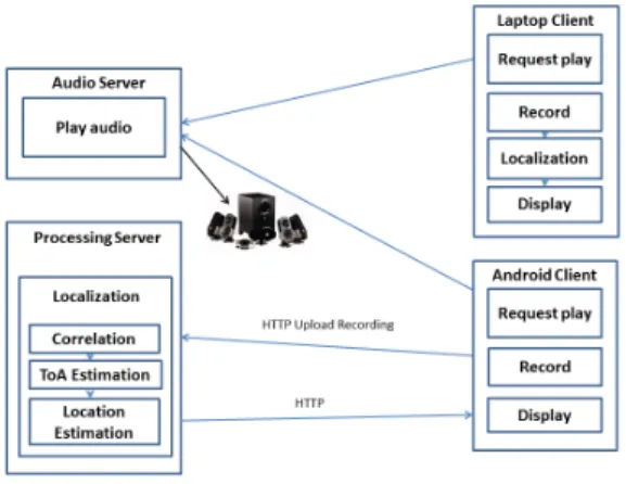
The first mode we experimented with is the request-play-record mode. A client requests that the server play known signals from each speaker, and the client then records its microphone signal. The recorded signal is processed, either on the client, or in the case of an Android client, is uploaded to a processing server. Finally, the result is returned to the client, for display on a map. This usage scenario is shown in Figure 3. In this case, although there is a rough level of synchronization in the sense that the latency between client requests and audio playing, may be on the order of .1 sec or less, we do not assume precise sample level synchronization. Synchronization is discussed in more detail below. For some scenarios, it may be appealing for clients to be able to request when sounds are to be played, but it has some disadvantages. One is the requirement of additional infrastructure and system complexity. Another is contention, since in a busy environ-ment, different clients may request sounds to be played at similar times.

Fig. 3. Request-play-record client-server mode. Clients make play requests to audio server. The server plays audio, and clients record audio. Clients then process audio locally, or upload to a server which processes recording and returns location estimates. The audio server and processing server may be the same machine.

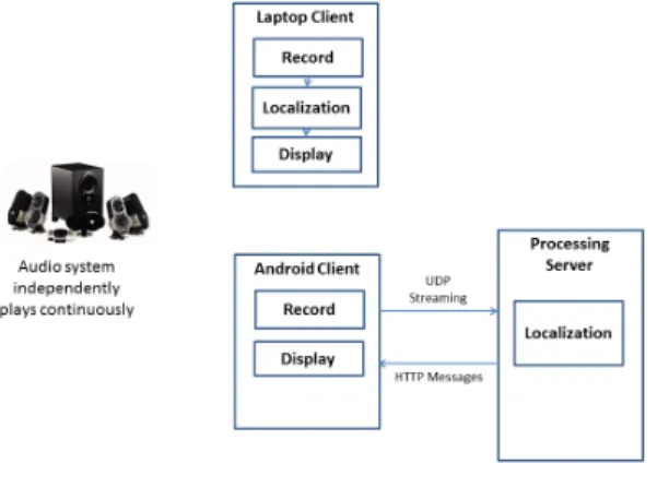
A second mode, with many advantages in practice, is continuous mode. In this mode, the signals are played con-tinuously, independently of any client requests. The signals played contain periodic pseudo random sequences, with period of about .5sec. In some cases we mix those signals with other sounds, such as music, which seem to have relatively little effect on the performance of the system. Note that for this mode, there is no a priori synchronization between player and client, and in fact the player does not require a server. We have successfully used an Oppo BDP-93 Blue-ray disc player for this purpose. Also, in this mode, the clients are running independently of the server and of each other. A client simply records some audio, and processes it, when it wants a localization. Note that in this mode, there is no single discrete signal. Although the processing may be performed on a single fixed length recording, it may also be performed continuously as a sort of position tracker. In the continuous case, successive audio buffers are used to estimate arrival delays, as peaks in a running average windowed correlation. Position estimates are recomputed each frame. An implementation of this continuous tracker will be discussed in Section IV-E.

Several important issues of synchronization and timing must be addressed in our system. All clients and servers have software accessible system clocks. In addition, there are sampling clocks used by all playing and recording audio devices. It is not easy to ensure synchronization of system clocks, because Android devices do not directly support an accurate time protocol such as NTP without ‘unlocking’ the devices to gain root privileges. It is also difficult to ensure syn-chronization between system clocks and audio device clocks, because the audio device interfaces typically do not provide the system clock time associated with the first sample of each audio buffer. We have found, and others have reported [11], unpredictable variable delays between system time and true sample time on the client side for various portable devices. On the server side, even using a low latency audio interface

Fig. 4. Continuous play mode. The audio system continually plays the signal, and various clients record independently, and process locally or stream to server for processing.

such as PortAudio [26] with ASIO drivers on Windows we found unpredictable delays. Consequently, we have adopted the strategy of treating the time delay between sample clocks of the playing and recording devices as an unknown to be solved for as part of the position estimation procedure. If signals are played at sample time 0 of the playing device, we associate this with sample timet0of the recording device,

and treat t0 as unknown. Similarly, we found that even the

relative clock rates differ and should be estimated.

Fortunately we found that clock drift remains consistent between pairs of devices, and also that within a given playing and recording ’session’ (i.e. in which the audio devices are started and buffers are maintained without overflow and under-flow) that synchronization is consistent for an extended time on the order of many minutes or even hours. Consequently, when our client software initiates audio capture, it records the system clock time as a ’session id’ and associates with each buffer filled by the audio device, the number of buffers filled, and the corresponding number of samples, since the beginning of that session. Even if the buffers are not all used, this maintains synchronization. This requires that buffers are accepted from the audio interface at a sufficient rate to avoid overflow. We found that using the Android AudioRecord Java interface, samples would sometimes be dropped. Even some Audio Recording Apps show this problem - that over the course of a long recording, samples would sometimes be dropped. We found that by using the native JNI OpenSL interface, this was avoided.

IV. LOCALIZATION

The basic methods of localization for both the request-play-record and the continuous variations of the server-client architectures discussed above are similar. Assume that sounds from all speakers are played starting at timet0and that sound

from speaker i reaches the microphone at timeti. Ifc is the speed of sound, (x, y, z)the position of the microphone and

(Xi, Yi, Zi)the position of speaker i, the propagation delays

ti−t0and distancesdi between speakers and microphone are

related by

di=c(ti−t0) = p

(x−Xi)2_{+ (y−Yi)}2_{+ (z−Zi)}2 ₍₁₎

There is a distinct such equation for each speakeri. The arrival timestiof the signals can be estimated using correlation meth-ods as described in Section IV-A. The remaining unknown quantities are the microphone position (x, y, z)and the time t0 at which all signals start playing. Methods for determining

these are described in Section IV-D.

Once the server receives the recorded audio file, it performs the following steps.

1) Perform cross-correlation of the recording with each reference signal.

2) Detect peaks in the cross-correlation withi-th reference signal to determine the time of arrival (ToA) at which sound from speakeri reached the recording device. 3) Estimate the location based on these determined time of

arrivals (ToAs).

4) Respond back with the estimated location to the client. A. Determining Time of Arrival (ToA)

If we model the impulse response between speaker i and the microphone as a weighted delta function shifted by the propagation delay, the signal at the microphone is

r(t) =X

i

wisi(t−τi) +η(t) (2) werewi is attenuation of signalsi(t)at the microphone,τi= ti−t0= d_ci is the time for sound from speaker ito reach the

microphone, andη(t)is additive noise.

The signal arrival times can be estimated using cross correlation or related methods. The cross correlation between signalssi andsj is defined as

Rij ≡Rsi,sj(τ)≡

X

t

si(t)sj(t+τ) (3) By linearity, the cross correlation of the signal si played at speaker iwith the recorded signal ris

Rs_i,r(τ) =

X

j

wjRs_i,sj(τ−τj) +Rsi,η(τ) (4)

Ifsi(t)are selected so that

Rsi,si(0) >> Rsi,si(τ) (τ 6= 0) (5)

Rs_i,si(0) >> Rsi,sj(τ) (i6=j) (6)

Rs_i,si(0) >> Rsi,η(τ) (7)

then Rsi,r(τ) will have its largest peak at τi, and τi =

arg maxτ Rsi,r(τ). We have used pseudo-random white noise

for the signalssi as it satisfies the above conditions well. In general, due to the presence of noise and multi-paths between a source and a receiver, general cross-correlation may not give distinctly identifiable peaks. This has been a topic of research for decades and variousgeneralized cross-correlation techniques have been developed [27]. These techniques incor-porate spectral weighting into the cross-correlation. Several

spectral domain weighting schemes have been proposed in literature and we have found good results using the Phase Transform (PHAT), defined as

RPHAT_s i,sj(τ) =F −1 _S∗ i(ω)Sj(ω) |S∗ i(ω)Sj(ω)| . (8)

Here, Si and Sj are the Fourier transforms of si and sj respectively, ∗ denotes complex conjugation, and ω is the frequency domain parameter. We have found PHAT to work much better than unweighted cross correlation, and although through this report we will useRsi,sj(τ)in our discussion, it

should be understood that typically we would use RPHAT si,sj(τ)

instead.

Note that in practice when we correlate si withr, we use the signal that was actually played, siˆ(t) defined such that

ˆ

si(0) is the first sample. Thensiˆ(t) =si(t+t0), and

ti= arg max

τ Rsˆi,r(τ) (9) These estimates are then used to solve for the microphone location, as described in Section IV-D.

B. Low-energy long duration signals

Equations 5, 6 and 7 put certain constraints on the audio signals that can be used for localization. These signals should be uncorrelated with each other and also with lagged copies of themselves. As such, naturally occurring sounds cannot be used for this purpose. One good candidate signal is pseudo-random noise sequence. However, we cannot play such signals aloud in an environment as these are unpleasant to hear. Hence, these signals are played with very low intensity (energy) so that these are barely audible. We have found that these low-energy noise signals can be added to the usual music being played in the environment without degrading the perceptive quality of the music and yet being effective in localization, as long as the playing system does not introduce non-linear distortions.

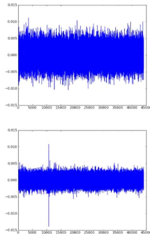
Although the use of barely audible signals allows us to use controlled signals for localization, their signal-to-noise ratio is very poor. Therefore, we play these signals for a long duration. Cross correlation between these long signals and their recordings improves the signal to noise ratio significantly. Figure 5 demonstrates this improvement where we show the cross-correlation of a 1-second long recording with a 1 second long reference signal, compared with a 10-seconds long recording correlated with a 10-seconds long reference signal. Longer duration correlations have much better correlation peaks. The overall localization accuracy also improves with longer recordings as shown in Figure 8 in Section V. C. Windowed cross-correlation

Since we want to use faintly audible sounds, the signal-to-noise ratio is not very high. As discussed in the previ-ous section, we overcome this limitation by using longer duration signal correlations. For a pseudo-random number sequencesi, the auto-correlation peak valueRi,i(0)increases linearly with the sequence length n, whereas the nonzero

Fig. 5. The top figure shows cross-correlation of recorded signal with 1 second long played signal. Bottom figure is the correlation between 10 seconds long recording with a 10 seconds long played signal. The 1-second long signals used for the top figure were generated by extracting only the first 1 second of both recorded and played signals. Correlations of longer duration signals show better peaks.

shift autocorrelation Ri,i(τ), τ 6= 0 and the cross-correlation Ri,j(τ), i6=jincrease sub-linearly (√n). Hence, using longer duration signals enhances peaks in the cross-correlation.

Since we compute cross-correlations using the FFTs of the signals (equation 8), it might be computationally wasteful to compute the FFTs of the entire lengths of the signal, if we are interested in only a small window of correlation lags (as is the case in the continuous tracker described in Section IV-E). Therefore, we divide the signals into smaller segments, and compute FFTs of only those segments which overlap with the other signal segments for the desired correlation lags.

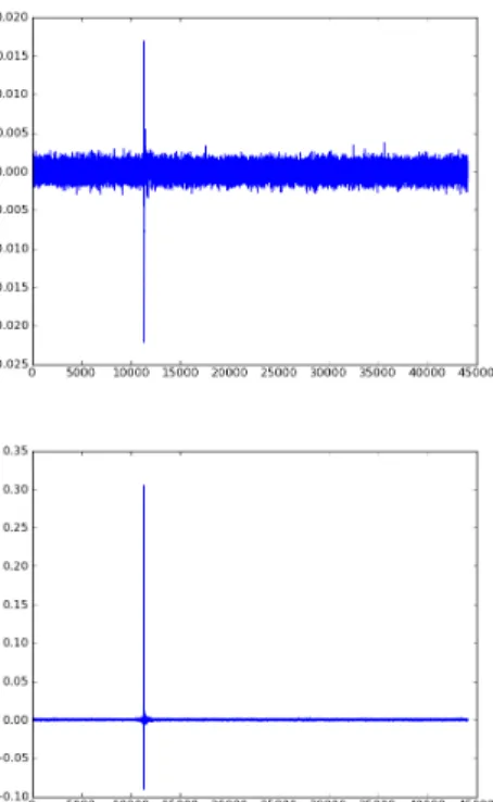
This windowed cross-correlation approach also helps in addressing another issue which we faced with long duration signals. Since the playback and recording devices have in-dependent clocks, there may be differences in their actual sampling rates which accumulate over time, resulting in a loss of synchronization and a poor correlation peak. The windowed scheme lets us take the mismatched clock speeds (also known as clock drift) into consideration, as would be discussed below. This can significantly increase the strength of peaks in correlation as shown in Figure 6 where we can see the remarkable improvement (by an order of magnitude) in the peak strength when clock drift is taken into account.

In the following discussion, we use the termsignalto refer to the played signal and denote it bys(t). The recorded signal r(t)is referred to as therecording.

Fig. 6. Top figure shows correlation of a 30s long recording with a 30s long reference signal without correcting the clock drift between the clocks of playing and recording devices. When the clock drift is taken into consideration (bottom figure), the cross-correlation shows remarkable improvement.

We divide s(t) into multiple segments, each of length G. The segments are referred to as s0, s1, ..., sM−1, where M is

the number of segments ins(t). The FFT length, denoted by F is determined as twice the next higher power of 2 than G, i.e., F = 2dlog2Ge+1_{. While taking the FFT of the signal’s} segments, p = F −G zeros are padded to each segment to make their length equal to F. The recording r(t) is also divided into multiple overlapping segments shifted by p, each of length F (except for the last one which may be smaller than F). These segments are labeled r0, r1, ..., rK−1, where

K is the number of segments in the recording.

Let Rsm,rk(τ) represent the correlation of m-th signal

segment with k-th recording segment for lag τ and Rsm,r

represent the correlation of sm with the whole recording. Rsm,rk is computed only for values of τ in the range 0 to

p−1, and is taken as 0 for otherτ. Then, Rsm,r(τ) = K−1 X k δ(m, k, τ)Rsm,rk(τ−kp) (10) Rs,r(τ) = M−1 X m Rs_m,r(τ+mG) (11) δ(m, k, τ)is 1 ifm-th signal segment overlaps with record-ing segmentrk for lagτ, otherwise it is 0. Assuming we want to find the cross-correlation for lags between τ1 andτ2, we

can avoid computing correlations between segments that do not overlap for any desired lag between [τ1, τ2].

1) Accounting for clock drift: Iffsandfmare the sampling rates of speakers system and microphone system respectively, thendrift rateis defined asα=fm

fs. To correct for clock drift,

the final accumulation of windowed correlations (equation 11), is modified as

Rs,r(τ) =

X

m

Rsm,r(τ+mαG) (12)

Note that if there is no clock drift, α = 1 and equation 12 reduces to equation 11.

2) Estimating clock drift: The drift rate needs to be deter-mined only once per recording device. We place the recording device very close to one of the speakers through which a 10 seconds long white noise signal is played. The played signal is divided into multiple segments of equal length (say 4000 samples). For each segment, we correlate it with the recording and find the position of thestrongestpeak. This peak denotes where in the recorded signal the segment under consideration of the played signal starts. Since the microphone was kept close to the speaker, the strongest peak should be the direct path peak. If there is a clock-speed mismatch, the starting position of each segment in the recorded signal drifts. By fitting a straight line between the start sample numbers of multiple segments in the played signal (on X-axis), against their corresponding peak sample numbers in the recording (on Y-axis), we can find the drift rate as theslopeof the line.

3) Avoiding spurious peak detection: The first occurrence of a signal in the recording (ti in equation 1) is determined by finding the peak in the cross correlation between the signal and the recording. A challenge we encountered in this method was the presence of spurious peaks in the correlation output due to multi-path effects. Although this was not very frequent, we noticed that in some locations, the peak due to multi-path effect was stronger than the direct-path peak. Therefore, we could not always choose the strongest peak as the direct path peak. We avoided such false peak selection using the following procedure. Locate the strongest peak in cross-correlation and then check all values up to W samples before this peak. If any cross-correlation value is more than a certain threshold (β times the strongest peak), then select this value as the true peak. The value ofW is determined by the room dimensions. IfL is the maximum distance between any two points in the room, then W = L

cf, wheref is the sampling rate and c is the speed of sound. The value ofβ is determined empirically (0.7 in our experiments).

D. Location Estimation

Onceti is determined for each speaker, equation (1) has 4 unknowns -x,y,z andt0. Four (independent) equations are

required to determine these unknown quantities. Since each speaker provides one equation, at least 4 speakers are needed to determine all quantities.

(x, y, z, t0)by minimizing the following error function. f(x, y, z, t0) = X i [p(x−Xi)2_{+ (y−Yi)}2_{+ (z−Zi)}2 −c(ti−t0)]2 (13) Note that ift0is known, only three equations, and estimates of

ti for three speakers are needed. If in addition tot0,zis also

known (for e.g. by making an assumption about the height at which a smartphone is being held) only two ti (and hence 2 speakers) are needed to solve for position.

Although linear formulations are also feasible, these require more than 4 speakers to estimate the location. If all speakers are in the same plane (for example when all speakers are roof-mounted), a procedure specified in [11] can be used to estimate the parameters using 4 speakers by solving the following equation for each speaker pair (i, j).

(Xi−Xj)x+ (Yi−Yj)y+ (Zi−Zj)z −c2(ti−tj)t0= 1 2[(X 2 i −X 2 j) + (Yi2−Yj2) + (Zi2−Zj2)−c2(t2i −t2j)] (14) In practice, it is better to use more speakers than the minimum requiredprovidedthe speakers are neitheroccluded nor too faint with respect to the recording device. In our experiments, we found that using the ti estimates from all speakers usually gave bad localization results. We attribute this to speakers being occluded, or too far from the receiver. This was also observed by Lopeset al[11]. To overcome this, we define a speaker peak quality parameterqi (equation 15) for each speaker such that speakers with better quality have more pronounced peaks. Then we choose thebest nspeakers according to their qi scores.

qi= maxRr,si

σ(Rr,s_i) (15)

HereRr,siis the cross-correlation between the recordingrand

signal (si) from thei-th speaker andσ()denotes the standard deviation operator.

E. Continuous tracker

Initially, we developed a request-play-record localizer in which the client made a request to the server to play sounds from speakers, recorded those sounds and uploaded this recording to the server. The server analyzed the recording to determine the 4 unknowns discussed earlier - x, y, z andt0.

Encouraged by the results, we built a continuously tracker that could track a device over an extended period of time. This tracker makes an assumption that z is around 1.25m, as this is typically the height at which someone would hold a smartphone. The tracker GUI, shown in Figure 1, can also use the fact that t0 does not change for a recording device if

it keeps track of the samples recorded since the beginning of localization.

Periodic signals with periodT are played from all speakers. The recorded signal shows correlation peaks at lag values in

the interval [0, T). In order to process received data in real-time, it is important to get a good bound (sayτminandτmax) on correlation lag values within which the peaks would occur. To do that, initially the tracker searches for peaks over the entire period[0, T)in the correlation signal for each speaker. Once it finds the location of a strong peak in any of the correlations, it chooses a window around that peak as the defining[τmin, τmax]range. The size of this window depends on the room size (max propagation time within the room). With a block size of 4096 samples at 44.1kHz, the tracker can find an appropriate lag window in less than half a second. This is a one-time-per-session process, after which the device can be tracked in real-time.

Once the appropriate window has been determined, the algorithm in Figure 7 is used to continuously determine the location. The subroutinenonlin_xyt0() in line 9 takes as input speaker positions (Pi, i = 1. . . N), determined peaks ({ti}), approximate value ofz and number of speakers to use (4, here) to estimatex,y andt0. It also returns aresidueres

which is the value of the error function defined in equation 13. We have found that this residue is a good indicator of how good the solution is. If the residue is small, the determined location is usually very close to actual location. A large residue indicates that the solution might not be correct. For this to work, we need to use one more speaker than the number of unknowns being estimated. We shall discuss this further in results section. bestSpeakers (line 15) takes the number of best speakers required, along with speaker positions and speaker qualities (equation 15) and returns a subset of the speaker positions to be used for localization.

If we find a good solution, we remember the value oft0as

t∗₀. If, later, nonlin_xyt0() does not find a good solution with 4 speakers, we use the saved value oft∗₀innonlin_xy() (line number 16) to estimate xandy with 3 speakers.

V. EVALUATION

We tested our approach in a meeting room of size 20ft ×

17ft × 8.5ft. 6 ceiling-mounted ordinary PC speakers were installed (shown as red circles in Figure 1). The room is moderately occupied by a set of desks, chairs and large TV screens, and was not modified in any way for our system beyond the installation of audio equipment. Two different approaches were evaluated. In the first approach, request-play-recordlocalizer, an Android app deployed on a Google Nexus S smartphone was used as the receiver. The app recorded audio and uploaded it to a pre-configured server over Wi-Fi. The audio level was audible, but soft enough that visitors to the room might not be aware of it until it was pointed out to them. We used signals of two different durations - 2 seconds and 10 seconds long. These signals were pseudo-random numbers uniformly sampled in the range -25000 to 25000 using Python SciPy’s random library and were white over the frequency range 0-22.05 KHz. 20 points distributed roughly uniformly within the room were chosen as ground truth. Localization was attempted 3 times at each of these points. Figure 8 shows that the localization accuracy was within 1 meter almost 80%

Input: Speaker positionsPi; played speaker signalssi; approximate height of microphonez; peak window size W; peak threshold pth; residue thresholdrth, speed of soundc

Initialize: t∗ 0=null 1

while truedo 2

r(t)←new recorded signal

3 Rsi,r(τ)←cross-correlation of r(t)withsi(t) 4 {pi} ←detectPeaks(Rs_i,r(τ),W,pth) 5 {qi} ← { maxR_si,r

standard deviation ofR_si,r}

6 {ti} ← {pi c} 7 {P_i4},{t4_i} ←bestSpeakers({Pi},{ti},{qi},4) 8 {x, y, t0},res←nonlin_xyt0(Pi4,{ti}, z) 9 if res < rth then 10 Outputx,y,z 11 t∗ 0←t0 12 else 13

if t∗₀ not nullthen 14 {P3 i},{t3i} ← 15 bestSpeakers({Pi},{ti},{qi},3) {x, y},res←nonlin_xy(P3 i,{ti}, z, t∗0) 16 if res < rth then 17 Outputx,y,z 18 end 19 end 20 end 21 end 22

Fig. 7. Periodic tracker algorithm.

of the times for the 10s long signals. 2s long signals did not perform as well as the 10s signals. Also compared are the performance using the best 4 speakers (as per equation 15) against performance using all 6 speakers.

We also developed a continuous tracker, as discussed in section IV-E. Its performance was evaluated using a Blue Microphones YETI mic connected to a laptop running a client developed in Python. For each ground truth position, the client requested localization around 200 times (each request was an audio recording of 4096 samples at 44.1 kHz). Figure 1 shows a snapshot depicting the localized mic (green dot). The green lines show the speakers used for localization in that step. Performance results are computed for all points put together. Table I shows how various methods perform for aresidue(res

as defined in Figure 7) threshold (rth) of 0.01 (determined empirically) and accuracy within 50cm (eth). Figure 9 shows localization accuracy for different types of estimators used in continuous tracking.

In this evaluation, apart from the linear solvers, we tested several non-linear location estimation methods based on the error function in equation 13. We would call the linear solvers

lin_best4(using best 4 speakers) andlin_all(using all 6 speakers) subsequently. The non-linear methods are named

nonlin_xyt0_X. The X refers to the number of speakers

Fig. 8. Location estimation accuracy of linear estimators for request-play-recordlocalizer. It is evident that performance is better using longer duration signals and recordings. Also note that using the best few speakers gives better accuracy than using all speakers.

used for localization: 3, 4, 5 and 6 in this case, respectively. These subroutines correspond to the algorithm in Figure 7 with lines 13 through 20 removed. We also tested the full algorithm (referred to ashybridfor subsequent discussion). In each of these evaluations, we assumed the height of the microphone to be around 1.25m from the ground. The only unknowns to be estimated werex,y andt0.

From the results, we can make the following observations. Localization accuracy does not always improve with more speakers, as discussed in section IV-D. Solvers using 3 or 4 speakers consistently performed better than the solvers using 5 or 6 speakers. The non-linear method with 3 speakers performs the best, localizing within 20cm 94% of the times. However, there is a non-zero chance (0.18%) of selecting a bad solution even with low residue (see the second data column in Table I). The non-linear method with 4 speakers also does well; not as well as the method with 3 speakers, but it has the advantage that a low value of residue is consistently indicative of a

TABLE I

PERFORMANCE(%)OF VARIOUS METHODS FOR RESIDUE THRESHOLD (rth)OF0.01AND ERROR THRESHOLD(eth)OF0.5M(I.E.,

LOCALIZATION ACCURACY OF0.5M OR BETTER).

Method r < rth r < rth r > rth r > rth e < eth e > eth e < eth e > eth lin best4 82.5 17.5 0 0 lin all 0 0 52.7 47.3 nonlin xyt0 3 94.02 0.18 0 5.8 nonlin xyt0 4 83.26 0 0 16.74 nonlin xyt0 5 76.92 0 0.24 22.84 nonlin xyt0 6 33.17 0 1.43 65.4 hybrid 83.62 0 0 16.38

Fig. 9. Location estimation accuracy of various estimators for continuous localizer (tracker) .

good solution. Finally, the hybrid method marginally improves upon the accuracy of the nonlinear method with 4 speakers. This improvement comes when nonlin_xyt0_4 fails to determine a good solution and the system uses a previously determined good estimate oft0to solve for justxandy(lines

13 to 20 in the algorithm shown in Figure 7. VI. DISCUSSION

Since in the tracker, z is set to be 1.25m, only x, y and t0 are estimated during localization. If x,ˆ yˆ and tˆ0

are the values estimated by a non-linear solver, then the

residue= f(ˆx,y, zˆ = 1.25,tˆ0). Using just 3 speakers to

determine the 3 unknowns, the residuewould typically be zero (if a numerical solution consistent with theti’s is found) even though this solution may be inaccurate due to errors in the estimates ofti.

Hence, with 3 speakers, if residue is small, there is no guarantee that the obtained solution will be correct. How-ever, if we use 1 additional speaker, then a low residue

would indicate a good solution. As can be seen in Table I, the probability of selecting a bad solution (e > eth)

for a low residue is 0 when we use 4, 5 or 6 speakers (nonlin_xyt0_X, X= 4,5,6), but is non-zero if 3 speak-ers are used (nonlin_xyt0_3). Therefore, we recommend

using one additional speaker than the number of unknowns to be determined. However, care should be taken that none of the speakers should get occluded, or be very far from the receiver. Thespeaker quality defined in equation 15 helps in selecting the appropriate speakers.

VII. CONCLUSION ANDFUTURE WORK

We have implemented an audio-based indoor localization system using low-energy pseudo-random sequences played through ordinary speakers. While determining ToAs, in order to improve signal-to-noise ratio, long duration sequences were used. To speed-up the computation of cross-correlation (by not computing cross-correlation for lags which are not required), windowed-cross-correlation was used. It also allows us to com-pensate for any clock drifts between the playing and recording devices. Our system has been implemented in multiple zones across our office building and is now a component of a system in constant operation. Evaluations in an actual meeting room demonstrate the efficacy of our approach.

There are several aspects which we would want to ex-periment with in the future. As of now, the speakers play pseudo-random sequences. We also tried adding this noise sequence to a music track such that the noise was barely perceptible against the music. Experiments using this noisy reference signal looked promising and we would like to test and evaluate this in real world settings. A variation would be to design signals which incorporate the random sequences in such a manner to allow higher power as part of naturally pleasing sounds like running water, ocean waves, waterfalls, and so on.

REFERENCES

[1] K. Chintalapudi, A. Padmanabha Iyer, and V. N. Padmanabhan, “Indoor localization without the pain,” inProc. 16th annual intl. conf. on Mobile computing and networking. ACM, 2010, pp. 173–184.

[2] E. Martin, O. Vinyals, G. Friedland, and R. Bajcsy, “Precise indoor localization using smart phones,” in Proc. intl. conf. on Multimedia, 2010, pp. 787–790.

[3] A. Varshavsky, E. de Lara, J. Hightower, A. LaMarca, and V. Otsason, “Gsm indoor localization,”Pervasive Mob. Comput., vol. 3, pp. 698–720, 2007.

[4] R. Want, A. Hopper, J. Falcao, and J. Gibbons, “The active badge location system,”ACM Trans. Inf. Syst., vol. 10, pp. 91–102, 1992. [5] J. R. Guerrieri, M. H. Francis, L. E. Miller, and et al., “RFID-Assisted

Indoor Localization and Communication for First Responders,” inThe European Conf. on Antennas and Propagation: EuCAP 2006, vol. 626, 2006.

[6] H. Kawaji, K. Hatada, T. Yamasaki, and K. Aizawa, “Image-based indoor positioning system: fast image matching using omnidirectional panoramic images,” in Proc. 1st ACM intl. workshop on Multimodal pervasive video analysis, 2010, pp. 1–4.

[7] M. Quigley, D. Stavens, A. Coates, and S. Thrun, “Sub-meter indoor localization in unmodified environments with inexpensive sensors,” in Intelligent Robots and Systems (IROS), 2010 IEEE/RSJ Intl. Conf. on, 2010, pp. 2039–2046.

[8] J.-S. Hu, C.-Y. Chan, C.-K. Wang, and C.-C. Wang, “Simultaneous lo-calization of mobile robot and multiple sound sources using microphone array,” inProc. 2009 IEEE intl. conf. on Robotics and Automation, 2009, pp. 4004–4009.

[9] W.-K. Ma, B.-N. Vo, S. Singh, and A. Baddeley, “Tracking an unknown time-varying number of speakers using tdoa measurements: a random finite set approach,”IEEE Trans. on Signal Processing, vol. 54, pp. 3291 – 3304, 2006.

[10] M. S. Brandstein, J. E. Adcock, and H. F. Silverman, “A practical time-delay estimator for localizing speech sources with a microphone array,” 1995.

[11] C. V. Lopes, A. Haghighat, A. Mandal, T. Givargis, and P. Baldi, “Localization of off-the-shelf mobile devices using audible sound: ar-chitectures, protocols and performance assessment,”SIGMOBILE Mob. Comput. Commun. Rev., vol. 10, pp. 38–50, April 2006.

[12] A. Mandal, C. Lopes, T. Givargis, A. Haghighat, R. Jurdak, and P. Baldi, “Beep: 3d indoor positioning using audible sound,” inProc. Consumer Comminucations and Networking Conference (CCNC), 2005, pp. 348– 353.

[13] J. Adcock and J. Foote, “Systems and methods for microphone local-ization,” Patent US 2005/0 249 360 A1, 11 10, 2005.

[14] T. Janson, C. Schindelhauer, and J. Wendeberg, “Self-localization appli-cation for iphone using only ambient sound signals,” inProc. Intl. Conf. on Indoor Positioning and Indoor Navigation (IPIN), 2010, pp. 1–10. [15] C. Peng, G. Shen, Y. Zhang, Y. Li, and K. Tan, “BeepBeep: a high

accuracy acoustic ranging system using COTS mobile devices,” inProc. 5th intl. conf. on Embedded networked sensor systems. ACM, 2007, pp. 1–14.

[16] B. Denby, Y. Oussar, I. Ahriz, G. Dreyfus, U. Pierre, and C. Paris, “Unsupervised indoor localization,”Architecture, pp. 1–5, 2010. [17] S. Tarzia, “Acoustic sensing of location and user presence on mobile

computers,” Ph.D. dissertation, Department of Electrical Engineering and Computer Science, Northwestern University, 2011.

[18] S. Tarzia, P. Dinda, R. Dick, and G. Memik, “Indoor localization without infrastructure using the acoustic background spectrum.” ACM, 2011.

[19] A. Harter, A. Hopper, P. Steggles, A. Ward, and P. Webster, “The anatomy of a context-aware application,” inProc. 5th annual ACM/IEEE intl. conf. on Mobile computing and networking, 1999, pp. 59–68. [20] M. Alloulah and M. Hazas, “An efficient cdma core for indoor acoustic

position sensing,” inProc. intl. conf. on Indoor Positioning and Indoor Navigation (IPIN), 2010, pp. 1–5.

[21] M. Hazas and A. Ward, “A high performance privacy oriented system,” in Proc. First IEEE intl. conf. Pervasive Computing and Communica-tions, 2003, pp. 216–223.

[22] C. Sertatl, M. Altnkaya, and K. Raoof, “A novel acoustic indoor localization system employing cdma,”Digital Signal Processing, vol. 22, no. 3, pp. 506 – 517, 2012.

[23] N. Mccouat and G. Brooker, “Broadband indoor acoustic location system,”System, pp. 609–614, 2005.

[24] E. Foxlin, M. Harrington, and G. Pfeifer, “Constellation: a wide-range wireless motion-tracking system for augmented reality and virtual set applications,” in Proc. 25th annual conf. Computer graphics and interactive techniques, 1998, pp. 371–378.

[25] N. Priyantha, A. Chakraborty, and H. Balakrishnan, “The Cricket location-support system,” in Proc. 5th intl. conf. (MobiCom). ACM, 2000, pp. 32–43.

[26] “Portaudio - an open-source cross-platform audio api,” //http://www.portaudio.com/.

[27] J. Chen, J. Benesty, and Y. Huang, “Time delay estimation in room acoustic environments: an overview,”EURASIP J. Appl. Signal Process., vol. 2006, pp. 170–170, January 2006.