UK real time macro data characteristics

BIROn - Birkbeck Institutional Research Online

Garratt, Anthony and Vahey, S.P. (2004) UK real-time macro data

characteristics. Working Paper. Birkbeck, University of London, London,

UK.

Downloaded from:

Usage Guidelines:

Please refer to usage guidelines at or alternatively

ISSN 1745-8587

Birkbeck Workin

g

Pa

p

ers in Economics & Finance

School of Economics, Mathematics and Statistics

BWPEF 0502

UK Real-Time Macro Data

Characteristics

Anthony Garratt

Shaun P Vahey

UK Real-time Macro Data Characteristics

∗

Anthony Garratt

Birkbeck College

Shaun P Vahey

Reserve Bank of New Zealand

December 21, 2004

Abstract

We characterise the relationships between preliminary and subsequent mea-surements for 16 commonly-used UK macroeconomic indicators drawn from two existing real-time data sets and a new nominal variable database. Most preliminary measurements are biased predictors of subsequent measurements, with some revision series affected by multiple structural breaks. To illustrate how thesefindings facilitate real-time forecasting, we use a vector autoregresion to generate real-time one-step-ahead probability event forecasts for 1990Q1 to 1999Q2. Ignoring the predictability in initial measurements understates con-siderably the probability of above trend output growth.

Keywords: real-time data, structural breaks, probability event forecasts

JEL Classification: C22, C82, E00

∗_{We thank Alex Brazier, Dean Croushore, Colin Ellis, George Kapetanios, Simon van}

1

Introduction

In this paper, we characterise the revisions to a variety of commonly-used UK

macro-economic indicators. We find that the preliminary measurements of most real-side

macro indicators are downwards biased predictors of subsequent measurements (at

the sample means). Structural breaks affect the relationships between early and

later measurements for many variables.

Previous studies, including (among others) Symons (2001), Castle and Ellis (2002) and Mitchell (2004) have noted the predictability property for the expendi-ture measure of output and its components. These (combined) studies characterise a subset of the indicators considered in this paper and provide no formal analyses of structural breaks. We use the Bai and Perron (2003a and 2003b) test for multiple breaks of unknown timing to examine the time variation in predictability.

Some of the UK indicators characterised in this study are drawn from two existing real-time data sets, Castle and Ellis (2002) and Egginton, Pick and Vahey (2002). Only Castle and Ellis (2002) characterise the revisions processes in detail (for the expenditure measure of output and its components). In addition, we analyse the

real-time quarterly monetary aggregates, nominal GDP and price deflator variables

neglected in the existing databases. The preliminary measurements of UK monetary aggregates are largely unbiased. In contrast, initial nominal GDP and GDP price

deflator measurements typically understate final measurements. The revisions to

these nominal variables rarely exhibit structural breaks. The untypical behaviour of

monetary aggregate revisions reflects the very different collection processes for these

series.

Macro models often perform better with revised data than with preliminary mea-surements. Real-time data sets allow researchers to condition their ex post model analyses on the information set actually available to forecasters and policymakers in real time. But if researchers ignore the predictability in initial measurements,

real-time model performance can be misjudged. We illustrate this with a specific

forecasting example. We use a vector autoregression (VAR) in UK real output

growth and inflation to forecast the (one-step ahead) probability of above trend

growth–sometimes referred to as the likelihood of “positive momentum”. Ignoring the predictability in initial measurements understates the event probability consid-erably for our 1990Q1 to 1999Q2 evaluation period.

The remainder of the paper is organised as follows. In section 2, we discuss the sources of UK real-time data. We describe our methodology for characterising UK real-time data in section 3 and report the main results in section 4. We analyse our illustrative probability forecasting VAR exercise in section 5. Section 6 concludes.

2

Data sources

Two on-line real-time UK data sources have appeared in the last couple of years:

Castle and Ellis (2002) and Egginton, Pick and Vahey (2002).1 _{Both studies adopt}

1

the standard terminology used in the more recent literature to describe the data (see, for example, Diebold and Rudebusch (1991)).

Typical macro databases store each time series variable as a column (or row) vector. In the real-time data literature, the remeasurements are recorded as succes-sive column vectors, and the data for each variable are usually stored as a matrix. The “vintage date” refers to the release date of each vector of time series measure-ments and the “vintage” denotes the column vector of time series data. Real-time data comprises many vintages; each successive column vector represents a vintage containing the data available at that vintage date. The “most recent”, “current”

and “final” labels are used interchangeably to denote the column with the latest

vintage date. These are not the “true” measurements, however, since these will be revised subsequently too.

Some researchers, including Egginton, Pick and Vahey (2002), use successive

vintages (columns) reflecting common practice by applied econometricians in

real-time policy and forecasting analyses. Others, including Howrey (1978) and Koenig et al (2003), use measurements that have been revised the same number of times (from the diagonals of the real-time data matrix for a particular variable).

Castle and Ellis (2002) provide the most comprehensive UK real-time data set.2

The variables comprise the expenditure components measure of real GDP (known as GDP(E)) in constant prices: private consumption, investment, government con-sumption, changes in inventories, exports, imports and GDP(E). The quarterly

sea-sonally adjusted variables were published initially by the Office for National

Sta-tistics (ONS) in Economic Trends and its Annual Supplement. An MS-Excel file

contains separate sheets for each variable. Following the standard conventions in

the literature, the columns reflect the vintages, with time series observations in the

rows. The first vintage refers to 1961Q1 and currently the last refers to 2003Q4.3

Since a typical quarter contains multiple vintages, the frequency of the vintage dates exceeds the frequency of the time series observations.

Egginton, Pick and Vahey (2002) provide additional real-time data for: GDP(O) (output measure of real GDP), private consumption, retail sales, government sur-plus, unemployment (total claimant count), M0, M3, M4, industrial production and

average earnings.4 The first two quarterly series and the remaining monthly

vari-ables came from the ONS publications Economic Trends and Financial Statistics.

Variables are downloadable individually in MS-Excel and ASCII text format. With the exception of the monetary aggregates, the sequence of vintages starts in January

1980 and ends in June 1999. For the monetary variables, M0, M3 and M4, thefirst

vintages are June 1981, January 1980 and June 1987 respectively, reflecting

avail-ability in the source publications. All variables are seasonally adjusted except the budget surplus. Unfortunately, the Egginton-Pick-Vahey data set contains no “deep history” information. The published versions of the original sources only show a (moving) window of data at any point in time. Empty cells denote data outside of that window–generally in excess of two years before the vintage date.

One concern for researchers interested in UK monetary issues is the absence

2_{Download fromhttp://www.bankofengland.co.uk/statistics/gdpdatabase.} 3

Annual updates occur in Spring of each year.

of quarterly monetary aggregates.5 To address this omission, we collected

real-time data on quarterly seasonally adjusted M0 and M4 from the ONS’ Economic

Trends for the vintages July 1987 to August 2002. We included (from the same

sources) additional real-time information on nominal GDP(E), GDP price deflator,

M0 velocity and M4 velocity. The interest in money velocity stems from its pivotal

role in the UK’s 1980’s monetary targeting experiments.6 For the last four variables,

the vintages start in November 1981 and end in 2002. Like the Egginton-Pick-Vahey data set, the absence of deep history results in some empty cells. The Appendix

contains more complete data descriptions.7

The causes of the UK revisions apparent in all three data sets are discussed in detail by Castle and Ellis (2002) and Mitchell (2004). In brief, revisions occur when the ONS receive new data, change their methodology or re-base variables. The new data category sometimes involves the substitution of delayed survey information for earlier judgement. The changes in methodology, associated with both the major

structural reforms, following the Pickford Report and the Chancellor’s Initiatives

(see Wroe (1993)), and other more minor reforms have unknown implementation dates. In contrast, the re-basing dates are known, and occur approximately every

five years. Unlike the other variables in our study, the monetary aggregate data were

collected by the Bank of England not the ONS. Topping and Bishop (1989) discuss

the definitions, collection of, breaks in and revisions to UK monetary aggregates.

3

Methodology

Our basic model for characterising UK remeasurements:

Y_tk = α + βX_tk + k_t, t= 1, . . . , T

(1)

where Y_tk =X_tF ₋X_tk defines the “revisions”, X_tF denotes the growth rate of the

“final” measurement andXk

t denotes thekth measurement of the growth rate of the

macro variable, k= 1, . . . , K where K < F. Notice that the preliminary

measure-ment on the right hand side predates the final measurement used to construct the

left hand side variable. The model corresponds to the “news” or “rational forecast”

specification analysed by (among others) Mankiw, Runkle and Shapiro (1984). The

null hypothesis of unbiasedness, α = 0 and β = 0, indicates unpredictable data

revisions. The orthogonality error condition of ordinary least squares ensures that

revision errors are uncorrelated with preliminary measurements.8

Since the indexk= 1, . . . , K denotes the successive measurements for each time

series observation, theXk

t variable is formed from many “vintages”: one data point

5_{The monthly seasonally adjusted monetary aggregates contained in Egginton, Pick and Vahey} (2002) were seasonally adjusted on a different basis from the quarterly equivalents for some of the period.

6_{See for example Jansen (1998). Although money velocities can be constructed from the} compo-nent variables, nominal GDP and the relevant monetary aggregates, we report the official measures for completeness.

7

The data are available in MS-Excel format on request from [email protected].

is taken from each vintage. In the results that follow, we restrict attention to the

k = 1 case for brevity. Results for the k= 2, . . . , K case can be obtained from the

authors on request.9 For the vector of “final” data,X_tF, we use the vintage available

from the ONS’ Economic Trends, 6 March 2003 (electronic version). A substantial

time interval exits between the respective sample end dates and the final vintage

date to allow revisions to occur.10

Our model could be extended to allow other macro indicators from the same

information set as Xk

t as explanatory variables (see, for example, Swanson and van

Dijk (2004)). Revisions are “efficient” if, and only if,α,β and the coefficients on the

additional explanatory variables are zero. Unfortunately, theory provides no

guid-ance on what other variables might be useful for testing efficiency and unrestricted

searches for predictability undoubtedly result in a degree of data snooping. In the absence of a theoretical basis for an examination of the predictability arising from

other variables, we prefer to test for bias–a sufficient (but not necessary) condition

for inefficiency–and test for multiple structural breaks.

Given the unknown implementation dates of some wide-ranging reforms to the UK data reporting processes (see Wroe (1993)), we adopt the methodology proposed by Bai and Perron (2003a and 2003b) to search for multiple structural breaks of

unknown timing.11 We introduce some additional notations to our basic revisions

equation (1):

Y_tk = αj + βjXtk + kt, t=Tj−1+ 1, . . . , Tj

(2)

for j= 1, ...., m+ 1. The linear regression hasm breaks (m+ 1 regimes) where the

indices (T1, ...., Tm)–the break points–are unknown, with T0 = 0 and Tm+1 =T.

So for the one break point case, m = 1 and j = 1,2, and the pair of estimated

parameters [α_b1,βb1] corresponds to the samplet= 1, ...., T1 and [αb2,βb2] corresponds

to the samplet=T1+ 1, ...., T. We define a break as a change in at least one of the

parameters αand β.

The Bai and Perron (2003a and 2003b) algorithm conducts efficient automated

searches for multiple breaks based on a dynamic programming approach. The

re-searcher chooses a maximum number of candidate breaks,N, and a trimming factor,

τ. Given these inputs the algorithm splits the sample into feasible sub-samples. The

maximised value of the residual sum of squares identifies the candidate breaks for

each number of breaks, n = 1, . . . , N. The researcher tests the null hypothesis of

no structural change against the alternative of many changes by a Sup Wald test.

Having identified at least one change, the number of breaks is identified by

specify-ing the null of n=L (1_≤L < N) changes againstL+ 1 changes and conducting a

sequence of SupF(L+ 1_|L) tests.

The Bai-Perron approach is robust to serial correlation and heteroskedasticity. Minor reforms to statistical reporting procedures could induce the latter and slow

9_{Contact [email protected]. We setK= 8 (16) for the quarterly (monthly) variables.} 10

We repeated our analysis reported below treating XtK as the final measurements. Although this limits the number of revisions allowed in each case the results were qualitatively similar. Again, the tables can be obtained from the authors on request.

adjustment by the agency would cause the former (see Barklem (2000)). Our ap-proach tests the stability of bias allowing for badly-behaved errors.

4

Characterising UK Revisions

4.1

Data

For our characterisations of UK data remeasurements we use sixteen variables in

total. Thefirst six variables are from the Castle-Ellis data set and comprise GDP(E),

consumption, investment, government expenditure, exports and imports, all for the period 1961Q3-1999Q2; the second six are from the Garratt-Vahey data set and

are nominal GDP and the GDP price deflator for 1981Q1-1999Q4, M0 and M4

for 1987Q1-1999Q4, M0 velocity for 1987Q1-1999Q4 and M4 velocity for

1986Q4-1998Q4; the final four are from the Egginton-Pick-Vahey data set and are average

earnings for 1979M11-1997M1, industrial production for 1979M11-1997M8, claimant count unemployment for 1979M12-1997M10 and retail sales for 1986M2-1997M12.

Since the indicators vary by source and time series frequency, the sample size,

the trimming factor τ (as a proportion of the sample) and the maximum number

of breaks, N, vary.12 We set N = 5 and τ = 0.15 for the 150 plus observations

for both the quarterly GDP(E) components in the Castle-Ellis data set and the

monthly indicators from Egginton-Pick-Vahey.13 For the Garratt-Vahey monetary

aggregates and velocities, where there are 52 or 53 quarterly observations, we set

N = 1 andτ = 0.25. For nominal GDP and the price deflator, there are 76 quarterly

observations and we set N = 2 and τ = 0.25.

We use quarterly or monthly growth rates as appropriate throughout the

empir-ical section.14 This approach mitigates the level effects that result from base year

changes (see Patterson and Hervai (1991)). In general, conventional unit root tests indicate that the variables in equation (2) are stationary, despite the small samples and the likely presence of structural breaks.

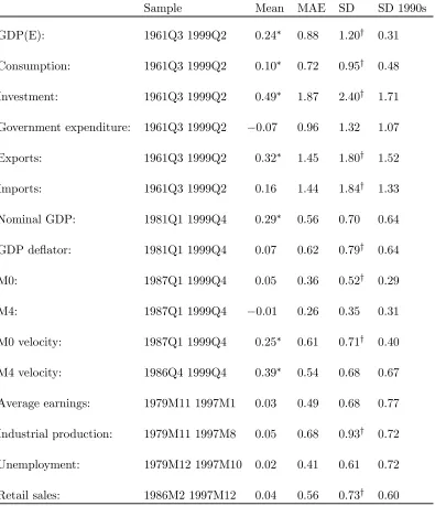
Table 1 reports the means and standard deviations of revisions, Y_t1. In

gen-eral, the mean revisions are positive: preliminary measurements understate final

measurements but there is considerable variation across variables. Approximately

half of the indicators have statistically significant mean revisions at the 5% level

(denoted by _∗ in Table 1). Investment has the largest (quarterly) mean revisions:

nearly twice as big as GDP(E).15 The notably small M0 and M4 mean revisions

are insignificantly different from zero at the 5% level. The mean absolute error for

the monetary aggregates is also notably lower than for the other variables. The preliminary analysis suggest little predictability for monetary aggregate revisions.

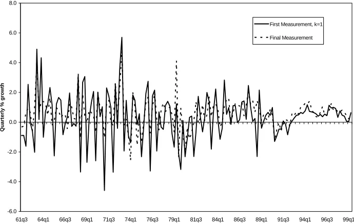
To illustrate the scale of revisions, Figure 1 plots GDP(E) from 1961Q3 to

1999Q2 for the first andfinal measurements. The deviation between the two shows

12_{Bai and Perron (2003b) discuss the appropriate parameter values in small samples.} 13

The Castle-Ellis data set contains (at times) more than one vintage per quarter. We used the vintage available at the start of each quarter and treated the Garratt-Vahey variables analogously.

14_{The growth rates forX}

twere defined as 100∗(logeXt−logeXt−1).

15

the k = 1 revision. At times, these are larger in absolute size than the quarterly

economic growth rate. Figure 1 also shows that the final measurements are much

less volatile post-1989, reflecting the relative stability of the 1990s boom.

-6.0 -4.0 -2.0 0.0 2.0 4.0 6.0 8.0

61q3 64q1 66q3 69q1 71q3 74q1 76q3 79q1 81q3 84q1 86q3 89q1 91q3 94q1 96q3 99q1

Qu

ar

te

rl

y

%

g

rowt

h

First Measurement, k=1

Final Measurement

Figure 1: GDP(E) Growth, First and Final Measurements

To check for structural change in the mean revision of each variable, we estimated

a restricted version of equation (2) with βj = 0. We used the Bai-Perron

method-ology to identify structural breaks of unknown timing in the intercept. There are

breaks in the means only for exports (1993Q3) and imports (1992Q1).16 _(The

re-sults reported in the next section based on unrestricted estimation of equation (2)

suggest that the data reject the βj = 0 restriction and that structural breaks are

much more prevalent.)

To investigate time variation in the standard deviations for each GDP(E) compo-nent, we split the sample into two sub-samples, corresponding approximately to the

1980s and 1990s.17 _{The results suggest a fairly consistent pattern: lower standard}

deviations for the 1990s. For 10 of the 16 variables, the data reject the null hypoth-esis of equal variances for the two sub-samples at the 5% level using a variance ratio

test (denoted by _† in Table 1).

We conclude from this preliminary investigation that revisions are often pre-dictable and typically positive, with considerable variation in size across variables and lower 1990s’ revision volatility.

16

The pre and post-break means were 0.23 (Newey-West coefficient standard error 0.091) and 0.81 (0.204) for exports and 0.02 (0.176) and 0.73 (0.219) for imports.

17

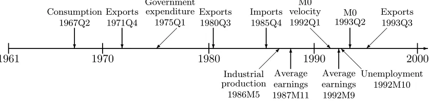
1961 1970 1980 1990 2000 @ @ R ? Consumption 1967Q2 ¡ ¡ ª Government expenditure 1975Q1 ? Imports 1985Q4 ? Exports 1971Q4 ? Exports 1980Q3 ¡ ¡ ª Exports 1993Q3 ? M0 1993Q2 -M0 velocity 1992Q1 6 Average earnings 1987M11 6 Average earnings 1992M9 ¡¡µ

Industrial production 1986M5 @ @ I Unemployment 1992M10

Figure 2: Break Points

4.2

Testing for Bias

Tables 2, 3 and 4 summarise the results from our regressions based on equation

(2) using 16 macro indicators for the first measurements (k = 1).18 In each case,

we report the p-value for the Wald test of the null hypothesis for unbiasedness,

α=β = 0, Newey-West heteroskedasticity and serial correlation consistent standard

errors and an LM-test statistic for serial correlation.19 _{The tables show the bias for}

each parameter-stable segment; if there are no structural breaks, we report the results for the full sample. The break points are also shown on a time line in Figure 2.

4.2.1 Castle-Ellis Variables

Table 2 reports the results for GDP(E) and its components. Most of these variables have breaks that pre-date the late 1980s’ and early 1990s’ structural reforms to ONS practices. The exports break in 1993Q3 coincides with the rebasing of national

accounts. In general, the null hypothesis of α =β = 0 can be rejected at the 1%

level, with variation in the size of the bias across variables. Initial measurements are

unfailingly revised upwards (at the sample means). For example, the estimated α

and β values for GDP(E) (investment) are in the region of 0.4 (0.6) and -0.6 (-0.3)

respectively. This implies preliminary GDP(E) (investment) measurements around the sample mean (quarterly) output growth of 0.4% (0.5%) would be revised to nearly 0.6% (0.9%). Nearly all variables subject to structural breaks display bias

before and after the breaks; the absolute values of the coefficients are sometimes

larger post-break. The null hypothesis of unbiased revisions can only be rejected in one sub-sample: for imports before the mid-1980s’ break.

18_{Tables for subsequent measurements (up to two years after the initial measurement) can be} obtained from the authors on request. Except for the monetary aggregates, the data reject the null hypothesis of unbiasedness for all kat the 1% level. However, the degree but not the direction of bias varies considerably withk.

19

4.2.2 Garratt-Vahey Variables

Table 3 reports the results for the six Garratt-Vahey nominal variables. With the exception of the early 1990s’ breaks for M0 and its velocity, these variables show stability over the period. Although nominal GDP revisions and the GDP price

deflator both exhibit significant bias at the 1% level, the monetary aggregates do not,

with p-values above 10% and smaller coefficients (in absolute value). The narrower

measure, M0, displays bias before the early 1990s’ break. In general, the revisions

to the money velocities are biased at the 1% level–reflecting the predictability of

nominal GDP revisions–with an early 1990s’ break for the narrower measure.

4.2.3 Egginton-Pick-Vahey Variables

Table 4 reports the results for the remaining four variables, all taken from the Eggington-Pick-Vahey data set. Both unemployment and industrial production have one break (in the early 1990s and mid-1980s, respectively); average earnings has two breaks (one in the late 1980s, the other in the early 1990s). In contrast, retail sales exhibits no breaks. In general, the preliminary measurements are downwards biased predictors of subsequent measurements at their sample means–matching the pat-tern observed for real-side quarterly indicators. The exceptions are unemployment,

average earnings and industrial production before their respectivefirst breaks. These

sub-samples display unbiasedness at the 15% level and above. All three indicators exhibit bias at the 1% level for subsequent sub-samples, consistent with statistical quality degradation.

4.2.4 Discussion

The predictability of revisions indicates the potential for improvements in UK sta-tistical quality. An agency aiming to minimise revisions could exploit revision

pre-dictability. However, filtering prior to data release can create difficulties for

mon-etary and fiscal control. In the absence of transparency, transformed preliminary

measurements severely complicate inferences about the data generating process

(Sar-gent (1989)).20

A statistical agency may prefer a less direct route to efficient revisions based on

gradual reforms to the quality of surveys and in-house estimates. The UK’s

well-known statistical reforms, associated with the Pickford Report and the subsequent

Chancellor’s Initiatives (see Wroe (1993)), had minor impacts on predictability. As

shown in Figure 2, only five structural breaks occurred in the 1989-1995 period.

For unemployment, predictability increased post-break. The monetary aggregates

produced by the Bank of England were unaffected by the reforms to ONS procedures.

Both exports and average earnings exhibit statistically significant predictability after

their early 1990s’ breaks.

Our preliminary analysis indicated that there was, however, some evidence that

the volatility of revisions fell after the Pickford Report. To check the robustness

20

of this characterisation in the presence of structural breaks, we tested for constant

variances across each break identified by the Bai-Perron approach. Using a variance

ratio test, the null of no difference in the variance can be rejected at the 5%, with

re-visions volatility lower post-break for most cases. The exceptions are unemployment and average earnings (second break).

5

Forecasting Case Study

Strong revisions predictability gives scope for improving real-time forecast perfor-mance. To illustrate this, we consider a probability event forecasting exercise.

We compute one step ahead out-of-sample forecasts for the evaluation period

1990Q1-1999Q2 using the unrestricted VAR estimated recursively:21

Xm_t =δm+

4

X

i=1

Γm_i Xm_t−i+εm_t

(3)

where Xm_t = (y_tm, pm_t )0, m = 1, F and B. The variables y and p denote quarterly

output growth and inflation (defined using the GDP price deflator). The superscript

m = 1, F and B denotes the set of first, final and bias-adjusted measurements

respectively. We define the bias-adjusted measurements, X_tB, as:

X_tB =α+ (1 +β)X_t1

(4)

where X_t1 denotes thefirst measurement. We assume that the forecaster knows the

true values of αand β and that they are equal to the respective sample coeficients

from equation (2).22

To arrive at our preferred specification for the forecasting VAR, we first tested

for stationarity and then selected the lag order. We could not reject the null of

a unit root in the levels data but could reject the null in first differences at the

5% level using augmented Dickey-Fuller tests (for both first andfinal measurement

data). We selected the lag order by estimating a sequence of unrestricted VAR(p),

p= 0,1,2, ...,6 models. For thefirst measurement data,m= 1, the optimal Akaike

Information Criteria selected lag length was zero; but forfinal data,m=F, the lag

order equalled four. Bearing in mind that unnecessary lags causes inefficiency but

not bias in the OLS estimators, we standardised the lag length at four forfirst,final

and the bias-adjusted data.

For model evaluation, we consider an economic agent monitoring business cycle turning points by calculating the probability of above trend output growth. This is sometimes referred to as “positive momentum” or “above speed limit” growth

in the monetary policy literature (Walsh (2003)). We take the (final data) average

economic growth rate for the evaluation period, 0.52%, as the “trend”, the agent

calculates the probability Pr[y_tm > 0.52_|Ωt−1], for m = 1, F and B where Ωt−1

denotes the information set dated t₋1. Confidence intervals are of limited help to

21

The sample start date reflects the availability of real-time GDP price deflator data.

our agent because the concern with turning points implies little interest in whether

any particular forecast confidence interval encompass a specific value for output.

Garratt et al (2003a) and Clements (2004) discuss in detail the appropriateness of

probability forecasts and their relationships to standard forecast confidence intervals.

We compute the probability forecasts by stochastic simulation by the methods

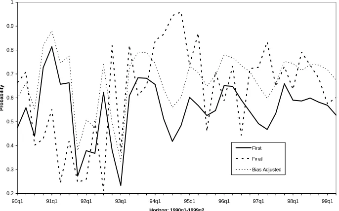
described by Garratt et al (2003b, appendix).23 Figure 3 plots the probabilities

of the event for the three data types. For most of the evaluation period, final

data results in a higher probability of above mean output growth than with first

measurement data. The average difference in probabilities is 11.6 percentage points

(with a standard deviation of 22.4%). Using bias-corrected measurements rather

thanfirst-measurement data reduces considerably the mean (absolute) difference in

forecast probabilities to 4.8 percentage points (with a standard deviation of 21.7%),

although substantial differences remain at times.

0.2 0.3 0.4 0.5 0.6 0.7 0.8 0.9 1

90q1 91q1 92q1 93q1 94q1 95q1 96q1 97q1 98q1 99q1

Horizon: 1990q1-1999q2

P

ro

b

a

b

ilit

y

First

Final

Bias Adjusted

Figure 3: One Step Ahead Probability of Above-trend Output Growth.

23

To obtain probability forecasts by stochastic simulation we simulate values of

Xm_T+1(s)=bδm(s)+ 4 X

i=1 b

Γmi X m(s) t−i +ε

m(s) T+1

where T runs from 1989Q4 to 1999Q1, the parameter estimates vary with each recursion, the superscript ‘(s)’ refers to thesthreplication of the simulation algorithm (s= 1,2, ....1000) and the

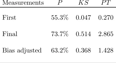
For more formal forecast evaluation, Table 5 reports the proportion of correctly

forecast events, P, the Kuipers score statistic, KS, and the Pesaran-Timmermann

(1992) directional market timing statistic, P T.

Table 5: Evaluation of probability event forecasts

Measurements P KS P T

First 55.3% 0.047 0.270

Final 73.7% 0.514 2.865

Bias adjusted 63.2% 0.368 1.428

We consider 38 events in total; one event (above trend growth) for each time period in the 1990Q1 to 1999Q2 evaluation period. We assume that an event can be correctly forecast if the associated probability forecast exceeds 50 percent. Although

over 70% of events can be correctly forecast usingfinal data, usingfirst measurements

and bias-adjusted measurements reduces the success rate by approximately 19 and 11 percentage points respectively.

The Kuipers scores also suggest that bias adjustment improves forecast perfor-mance. This statistic measures the proportion of above mean growth rates that were correctly forecast minus the proportion of below mean growth rates that were incorrectly forecast. The test provides a measure of the accuracy of directional

fore-casts, with high positive numbers indicating high predictive accuracy. Using first

measurements gives aKS of approximately 0.05; bias-adjustment betters this score

by 0.32 – considerably closer to the final data score of 0.51.

The P T statistic allows a formal hypothesis of directional forecasting

perfor-mance. As shown in Granger and Pesaran (2000), this hypothesis test uses the same information as the Kuipers score. Under the null hypothesis that the forecasts

and realisations are independently distributed the P T statistic has a standard

nor-mal distribution. Thefirst measurement data reject the null of no ability to forecast

oberved changes with a probability value of 0.78. Bias-adjustment reduces the prob-ability value to 0.15 – indicating rejection at the 15% level. Final data give clear rejection at the 1% level. We conclude that bias adjustment improves probability

forecasting performance for this particular forecasting example.24

24

Although this analysis indicates the scope for exploiting revision predictability, we emphasise that the variation in predictability across variables and through time

ensures that performance improvement is case specific. Furthermore, the parameters

of equation (2) were assumed to be known by the agent (and identified as the

pop-ulation coefficients). In the presence of structural breaks, parameter learning may

limit the scope for increasing forecast accuracy. Modelling the impacts of bounded rationality on real-time forecast and policy model performance is an interesting area for subsequent research.

6

Conclusions

By utilising both existing and new sources of real-time data, this paper has

charac-terised the revision processes for 16 UK macro indicators. The main finding–that

the preliminary measurements of UK macro variables are generally biased–confirms

a widely-held suspicion that UK macro measurements are inefficient. Where present,

References

[1] Bai, J., and P. Perron (1998) “Estimating and Testing Linear Models with

Multiple Structural Changes”, Econometrica, 66, 47-78.

[2] Bai, J., and P. Perron (2003a) “Computation and Analysis of Multiple

Struc-tural Change Models”,Journal of Applied Econometrics, 18, 1-22.

[3] Bai, J., and P. Perron (2003b) “Critical Values for Multiple Structural Change

Tests”,Econometrics Journal, 6, 72-78.

[4] Barklem, A. (2000) “Revisions Analysis of Initial Estimates of Key Economic

Indicators and GDP Components”,Economic Trends, 556, 31-52.

[5] Castle, J. and C. Ellis (2002) “Building a Real-time Database for GDP(E)”,

Bank of England Quarterly Bulletin, February, 42-49.

[6] Clements, M.P. (2004) “Evaluating the Bank Of England Density Forecasts of

Inflation”, Economic Journal, 114, 844-866.

[7] Croushore, D. and T. Stark (2001) “A Real-time Data Set for Macroeconomists”

Journal of Econometrics, 105, 111-130.

[8] Diebold, F. X., and G. D. Rudebusch (1991) “Forecasting Output with the

Composite Leading Index: A Real-Time Analysis”, Journal of the American

Statistical Association, 86, 603-610.

[9] Egginton, D.M., A. Pick and S.P. Vahey (2002) “ ‘Keep It Real!’ A Real-time

UK Macro Data Set”, Economics Letters, 77, 15-20.

[10] Faust, J., J.H. Rogers and J.H. Wright (2004) “News and Noise in G7 GDP

Announcements”, Journal of Money, Credit and Banking, forthcoming.

[11] Garratt, A., K. Lee, M.H. Pesaran, and Y. Shin, Y. (2003a)

“Fore-cast Uncertainties in Macroeconometric Modelling: An Application to

the UK Economy”, Cambridge University Discussion Paper, available at

http://www.econ.cam.ac.uk/faculty/pesaran.

[12] Garratt, A., K. Lee, M.H. Pesaran, and Y. Shin, Y. (2003b) “Forecast Uncer-tainties in Macroeconometric Modelling: An Application to the UK Economy”,

Journal of American Statistical Association, Applications and Case Studies, 98, 464, 829-838.

[13] Granger, C.W.J. and M.H. Pesaran (2000), “Economic and Statistical Measures

of Forecast Accuracy,” Journal of Forecasting, 19, 537-560.

[14] Howrey, E.P. (1978) “The Use of Preliminary Data in Econometric

Forecast-ing”,Review of Economics and Statistics, 60, 193-200.

[15] Jansen, N. (1998), “The Demand for M0 in the United Kingdom Reconsidered:

[16] Koenig, E., S. Dolmas and J. Piger (2003) “The Use and Abuse of ‘Real-time’

Data in Economic Forecasting”, Review of Economics and Statistics, 85,

618-628.

[17] Mankiw, N.G., Runkle, D.E and M.D. Shapiro (1984) “Are Preliminary

An-noucements of the Money Stock Rational Forecasts”,Journal of Monetary

Eco-nomics, 14, 15-27.

[18] Mitchell, J. (2004) Revisions to Economic Statistics, National Institute of

Eco-nomic and Social Research, April.

[19] Newey, W.K. and K.D. West (1987) “A Simple Positive Semidefinite,

Het-eroskedasticity and Autocorrelation Consistent Covariance Matrix”,

Economet-rica, 55, 703-708.

[20] Patterson, K. D., and S. M. Heravi (1991) “Data Revisions and the Expenditure

Components of GDP” Economic Journal, 101, 887-901.

[21] Pesaran, M.H. and A. Timmermann (1992), “A Simple Nonparametric Test

of Predictive Performance,” Journal of Business and Economic Statistics, 10,

461-465.

[22] Pickford S. (1989)Government Economic Statistics: A Scrutiny Report,

Cabi-net Office, HMSO.

[23] Rosenblatt, M. (1952) “Remarks on a Multivariate Transformation”, Annals of

Mathematical Statistics, 23, 470-472.

[24] Sargent, T., (1989) “Two Models of Measurements and the Investment

Accel-erator”,Journal of Political Economy, 97, 251-287.

[25] Swanson, N.R. and D. Van Dijk (2004) “Are Statistical Reporting Agencies Get-ting It Right? Data Rationality and Business Cycle Asymmetry”, Econometric Institute Report EI 2001-28, revised 2004.

[26] Symons, P. (2001) “Revisions Analysis of Initial Estimates of Annual Constant

Price GDP and Its Components”, Economic Trends, 568, 48-65.

[27] Topping, S.L. and S. L. Bishop (1989), “Breaks in Monetary Series” Bank of England Discussion Paper, Technical Series, No. 23.

[28] Walsh, (2003) “Speed Limit Policies: the Output Gap and Optimal Monetary

Policy”,Amercian Economic Review, 93, 265-278.

[29] Wroe, D. (1993) “Improving Macro-economic Statistics”, Economic Trends,

7

Appendix: Summary of Garratt-Vahey real-time data

In this appendix, we describe the real-time data collected specifically for this study

(referred to as the Garratt-Vahey data set in the main text). The data consist of monthly vintages of nominal macroeconomic variables. Each variable has many

different vintages–reflecting the revisions and updates that occur over time. In

the MS-Excel files, the data are stored as a matrix for each variable. Successive

column vectors of the matrix represent different (more recent) vintages of data; each

contains the most recent measurements available at that vintage date. The data were

collected by examining various issues ofEconomic Trends, which is published by the

ONS (formally the Central Statistical Office).

The figures reported were in the public domain at the end of the month in

question. For each vintage, the observations are identical to those in the relevant

published source. The window length reported by the source publications is affected

by page layout considerations–it varies by variable and by vintage date. Missing

data are recorded as empty cells. The two excel files containing the data described

below, nomY&Pdef.xls and money.xls, are available from the authors on request.

In the following section, the definition, source, code, period and relevant notes

are described for each variable.

1. Nominal GDP (Excel file: nomY&Pdef.xls, Spreadsheet: nominal mktp(sa)).

Definition:- Gross domestic product at market prices, current price$ Million, seasonally adjusted.

Source:- ONSEconomic Trends.

Code:- FNAM (from Nov 1981 to Sept 1985), CAOB (from Oct 1985 to Sept 1998) and YBHA (from Oct 1998 onwards).

Period:- Monthly vintages from Nov 1981 to August 2002, on quarterly obser-vations 1976Q1 to 2002Q1.

2. GDP price deflator (Excel file: nomY&Pdef.xls,Spreadsheet: deflator mktp).

Definition:- Implied market price deflator (average estimate).

Source:- ONSEconomic Trends.

Code:- DJDT (from Nov 1981 to Oct 1998) and YBGB (from Oct 1998 on-wards).

Period:- Monthly vintages from Nov 1981 to August 2002, on quarterly obser-vations 1976Q1 to 2001Q4.

3. M0 money (Excel file: money.xls,spreadsheet: M0 sa).

Definition:- M0,$ Million, Amount outstanding, seasonally adjusted.

Source:- ONSEconomic Trends.

Code:- AVAE.

4. M4 money (Excel file: money.xls,spreadsheet: M4 sa).

Definition:- M4,$ Million, Amount outstanding, seasonally adjusted.

Source:- ONSEconomic Trends.

Code:- AUYN.

Period:- Monthly vintages from July 1987 to August 2002, on quarterly obser-vations 1983Q1 to 2002Q1.

5. VM0 money (Excel file: money.xls,spreadsheet: V(M0)).

Definition:- Velocity of circulation.

Source:- ONSEconomic Trends.

Code:- AVAM.

Period:- Monthly vintages from July 1987 to August 2002, on quarterly obser-vations 1983Q1 to 2002Q1.

6. VM4 money (Excel file: money.xls,spreadsheet: V(M4)).

Definition:- Velocity of circulation.

Source:- ONSEconomic Trends.

Code:- AUYU.

Table 1: Summary Statistics for Revisions,

Y

Sample Mean MAE SD SD 1990s

GDP(E): 1961Q3 1999Q2 0.24∗ 0.88 1.20† 0.31

Consumption: 1961Q3 1999Q2 0.10∗ 0.72 0.95† 0.48

Investment: 1961Q3 1999Q2 0.49∗ 1.87 2.40† 1.71

Government expenditure: 1961Q3 1999Q2 ₋0.07 0.96 1.32 1.07

Exports: 1961Q3 1999Q2 0.32∗ 1.45 1.80† 1.52

Imports: 1961Q3 1999Q2 0.16 1.44 1.84† 1.33

Nominal GDP: 1981Q1 1999Q4 0.29∗ _{0.56 0.70 0.64}

GDP deflator: 1981Q1 1999Q4 0.07 0.62 0.79† 0.64

M0: 1987Q1 1999Q4 0.05 0.36 0.52† 0.29

M4: 1987Q1 1999Q4 ₋0.01 0.26 0.35 0.31

M0 velocity: 1987Q1 1999Q4 0.25∗ 0.61 0.71† 0.40

M4 velocity: 1986Q4 1999Q4 0.39∗ 0.54 0.68 0.67

Average earnings: 1979M11 1997M1 0.03 0.49 0.68 0.77

Industrial production: 1979M11 1997M8 0.05 0.68 0.93† _0.72

Unemployment: 1979M12 1997M10 0.02 0.41 0.61 0.72

Retail sales: 1986M2 1997M12 0.04 0.56 0.73† 0.60

Notes: The revisions,Y_t1, are defined as thefinal measurement,X_tF, minus thefirst

measurement, X1

t. Each measurement, Xt, refers to the quarter-on-quarter (first

12 variables) or month-on-month (last 4 variables) growth rate in percent. MAE is the mean absolute error; SD refers to standard deviation and SD 1990s refers to the

standard deviation for the 1990s. The symbol ∗ _{denotes statistical significance at}

the 5% level using a Newey-West corrected t-statistic based on a regression of the

revision on a constant. Significantly lower variance for the 1990s at the 5% level

Table 2: Revisions regressions, Castle-Ellis

Sample α β R2 Wald-test LM-test

GDP(E): 1961Q3 1999Q2 0.444 -0.573 0.58 0.00 0.30

(0.065) (0.050)

Consumption: 1961Q3 1967Q2 0.478 -0.682 0.64 0.00 0.86

(0.120) (0.087)

1967Q3 1999Q2 0.252 -0.288 0.20 0.00 0.00

(0.072) (0.051)

Investment: 1961Q3 1999Q2 0.563 -0.320 0.17 0.00 0.01

(0.147) (0.074)

Government 1961Q3 1975Q1 0.421 -0.591 0.24 0.01 0.17

expenditure: (0.185) (0.182)

1975Q2 1999Q2 0.181 -0.816 0.33 0.00 0.01

(0.083) (0.128)

Exports: 1961Q3 1971Q4 0.630 -0.237 0.43 0.00 0.13

(0.117) (0.032)

1972Q1 1980Q3 0.219 -0.068 0.01 0.34 0.03

(0.156) (0.077)

1980Q4 1993Q3 0.495 -0.525 0.45 0.00 0.00

(0.139) (0.063)

1993Q4 1999Q2 1.274 -0.458 0.25 0.00 0.43

(0.290) (0.159)

Imports: 1961Q3 1985Q4 0.156 -0.120 0.05 0.03 0.00

(0.130) (0.043)

1986Q1 1999Q2 0.920 -0.473 0.42 0.00 0.67

(0.290) (0.082)

Notes: Revisions regression, Equation (2), Y_t1 = αj +βjXt1 + 1t. Newey-West

standard errors (truncation factor equals 4) are in parentheses. We report p-values

of the Wald-test for α=β = 0 and the LM-test statistic for up to 4th-order serial

Table 3: Revisions regressions, Garratt-Vahey

Sample α β R2 Wald-test LM-test

Nominal GDP: 1981Q1 1999Q4 0.929 -0.431 0.27 0.00 0.22

(0.141) (0.097)

GDP deflator: 1981Q1 1999Q4 0.696 -0.595 0.30 0.00 0.16

(0.135) (0.078)

M0: 1987Q1 1993Q2 0.555 -0.494 0.50 0.00 0.09

(0.131) (0.078)

1993Q3 1999Q4 0.114 -0.035 -0.03 0.46 0.08

(0.077) (0.041)

M4: 1987Q1 1999Q4 -0.020 0.006 -0.02 0.97 0.16

(0.081) (0.030)

M0 velocity: 1987Q1 1992Q1 0.937 -1.040 0.72 0.00 0.97

(0.049) (0.190)

1992Q2 1999Q4 0.025 -0.538 0.48 0.00 0.26

(0.074) (0.114)

M4 velocity: 1986Q4 1999Q4 0.254 -0.141 0.04 0.00 0.91

(0.111) (0.80)

Notes: Revisions regression, Equation (2), Y_t1 = αj +βjXt1 + 1t. Newey-West

standard errors (truncation factor equals 4) are in parentheses. We report p-values

of the Wald-test for α=β = 0 and the LM-test statistic for up to 4th-order serial

Table 4: Revisions regressions, Egginton-Pick-Vahey

Sample α β R2 Wald-test LM-test

Average earnings: 1979M11 1987M11 0.108 -0.138 0.05 0.23 0.00

(0.072) (0.079)

1987M12 1992M9 0.464 -0.688 0.45 0.00 0.01

(0.091) (0.129)

1992M10 1997M1 0.257 -0.907 0.87 0.00 0.19

(0.028) (0.045)

Industrial 1979M11 1986M5 0.050 -0.033 -0.01 0.80 0.06

production: (0.081) (0.076)

1986M6 1997M8 0.103 -0.508 0.29 0.00 0.00

(0.047) (0.092)

Unemployment: 1979M12 1992M10 0.063 -0.026 0.00 0.42 0.00

(0.056) (0.30)

1992M11 1997M10 -0.428 -0.328 0.25 0.01 0.13

(0.154) (0.101)

Retail sales: 1986M2 1997M12 0.120 -0.390 0.41 0.00 0.00

(0.029) (0.042)

Notes: Revisions regression, Equation (2), Y_t1 = αj +βjXt1 + 1t. Newey-West

standard errors (truncation factor equals 4) are in parentheses. We report p-values

of the Wald-test for α=β = 0 and the LM-test statistic for up to 12th-order serial