Boundary Layer Transition on a Slender Cone in Hypervelocity Flow with Real Gas Effects

(1)

Hypervelocity Flow with Real Gas Eﬀects

Thesis by

Joseph Stephen Jewell

In Partial Fulﬁllment of the Requirements for the Degree of

Doctor of Philosophy

California Institute of Technology Pasadena, California

2014

(2)

2014 Joseph Stephen Jewell

(3)

(4)

Abstract

The laminar to turbulent transition process in boundary layer flows in thermochemi-cal nonequilibrium at high enthalpy is measured and characterized. Experiments are performed in the T5 Hypervelocity Reflected Shock Tunnel at Caltech, using a 1 m length 5-degree half-angle axisymmetric cone instrumented with 80 fast-response an-nular thermocouples, complemented by boundary layer stability computations using the STABL software suite. A new mixing tank is added to the shock tube fill appara-tus for premixed freestream gas experiments, and a new cleaning procedure results in more consistent transition measurements. Transition location is nondimensionalized using a scaling with the boundary layer thickness, which is correlated with the acoustic properties of the boundary layer, and compared with parabolized stability equation (PSE) analysis. In these nondimensionalized terms, transition delay with increasing CO2 concentration is observed: tests in 100% and 50% CO2, by mass, transition up

to 25% and 15% later, respectively, than air experiments. These results are consistent with previous work indicating that CO2 molecules at elevated temperatures absorb

acoustic instabilities in the MHz range, which is the expected frequency of the Mack second-mode instability at these conditions, and also consistent with predictions from PSE analysis. A strong unit Reynolds number eﬀect is observed, which is believed to arise from tunnel noise. NTr for air from 5.4 to 13.2 is computed, substantially higher

(5)

for the leading edge, centroid, and trailing edge of the spots. A model constructed with these spot propagation parameters is used to infer spot generation rates from measured transition onset to completion distance. Finally, a novel method to control transition location with boundary layer gas injection is investigated. An appropriate porous-metal injector section for the cone is designed and fabricated, and the eﬃ-cacy of injected CO2 for delaying transition is gauged at various mass ﬂow rates, and

compared with both no injection and chemically inert argon injection cases. While CO2 injection seems to delay transition, and argon injection seems to promote it, the

(6)

Acknowledgements

Joe Shepherd, my advisor, deserves credit for his careful guidance, expertise, and substantial patience over the years. I returned to Caltech speciﬁcally to work with him after getting my ﬁrst real research experience in his lab group as a summer SURF student in 2002, and have since only grown in my appreciation for this exceptional scientist and educator. Ivett Leyva of the Air Force Research Laboratory went above and beyond any reasonable expectation as a collaborator and committee member, regularly making the drive to Pasadena to discuss our work in person and advise on research and writing. The other members of my committee are Hans Hornung, Tony Leonard (who was also my undergraduate Aeronautics advisor), and Guillaume Blanquart, each of whom not only read the thesis but provided careful review of early drafts for a substantial portion of this work. Warren Brown (who was also my undergraduate Medieval History advisor) advised me on the coursework for the History minor.

(7)

collaboration improved the quality of the work described in this thesis, just as his friendship and softball-managing skills contributed to my enjoyment of my time at Caltech.

Running T5 is always a team eﬀort, and no experiments would have been possi-ble without the engineering and technical work of Bahram Valiferdowsi. Along with Bahram, Stuart Laurence and Eric Marineau patiently taught me how to run the facility during the early days of this work and were instrumental in learning to take and reduce T5 data. Amy Kar-Wei Beierholm’s early work with potential injection mechanisms was important for the development of the experimental section in Chap-ter 7.

Alexander Fedorov at the Moscow Institute of Physics and Technology reviewed the draft of Chapter 7 and was a fruitful collaborator from the earliest days of this work. Sasha’s 2011 lectures on hypersonic stability and transition were useful in the composition of Chapter 4.

Discussions on boundary layer stability with Neal Bitter were very helpful, espe-cially in the composition of Section 4.3.2 and in comparing his computations with STABL results. His friendship has been a blessing to me.

Elizabeth Jewell of the University of Michigan (Ann Arbor), my statistician sister, provided substantial advice on the statistical analysis in Section 5.3.

Bryan Schmidt helped perform the mass-ﬂow meter calibration shown in Fig-ure 7.3, and used that calibration to make porous media mass-ﬂow rate measure-ments.

(8)

Other members of the Shepherd group, including Phil Boettcher, Sally Bane, Angie Capece, Stephanie Coronel, Greg Smetana, and Remy Mevel each provided advice, support, and friendship.

I am also indebted to Christopher Brennen, whose courses were my formal intro-duction to fluid mechanics and have subsequently been instrumental to my efforts in the field. Chris also advised me and John Meier on the most interesting and fruitful side project I pursued during this work.

My parents, Suzanne and Stephen Jewell, along with my grandparents Dorothy Kramer and the late Charles and F. Kathryn Jewell, have been the basis for all of my success. My grandfather, Richard M. Kramer, to whose memory this thesis is dedicated, gave me my earliest experiences of engineering in his basement workshop, and remained an enthusiastic and curious supporter of my work for the rest of his life.

My wife Katie’s patient love and support has been critical to the completion of this work. I simply do not deserve her. Finally, thanks be to God for perseverance and fortitude: “O give thanks unto the _Lord; for he is good: for his mercy endureth forever.”1

This project was sponsored by the Air Force Office of Scientific Research under award number FA9550-10-1-0491 and the NASA/AFOSR National Center for Hy-personic Research. The author was supported by the National Defense Science and Engineering Graduate Fellowship, the Jack Kent Cooke Foundation Graduate Schol-arship, and the Boeing Fellowship. The views expressed herein are those of the author and should not be interpreted as necessarily representing the official policies or en-dorsements, either expressed or implied, of the sponsors, Caltech, AFOSR, or the U.S. Government.

Verbum Domini Manet in Aeternum

(9)

List of Figures

1.1 Fujii absorption/wavelength for air, N2, and 50% CO2 . . . 8

2.1 T5 rendering . . . 13

2.2 T5 simpliﬁed schematic . . . 13

2.3 Gas premixing tank . . . 15

2.4 Gas premixing tank fans . . . 16

2.5 T5 simpliﬁed schematic with transducers . . . 18

2.6 T5 burst pressure signals, shot 2742 . . . 20

2.7 T5 shock time signals, shot 2742 . . . 20

2.8 T5 reservoir pressure signals, shot 2742 . . . 22

2.9 Grid used for nozzle computations . . . 25

2.10 Shot 2742 turbulent wall nozzle ﬂow . . . 35

2.11 Shot 2742 laminar wall nozzle ﬂow . . . 36

3.1 Cone . . . 38

3.2 Cone tip . . . 39

3.3 Dimensional cone drawing . . . 40

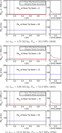
3.4 Re_kk distribution for three sample experiments . . . 42

3.5 Re_kk vs. Re_k, all shots . . . 43

3.6 Thermocouple layout . . . 46

3.7 Equilibrium and frozen adiabatic wall temperatures . . . 50

(17)

3.9 Shot 2744 Re vs. St plot . . . 57

3.10 Intermittency method . . . 59

3.11 a4/a1 vs. Ms for ideal tailored operation . . . 61

3.12 P4/P1 vs. hres for ideal tailored operation . . . 62

3.13 Shock speed decay in air, 84% He, 16% Ar driver, P4 ≈100 MPa . . . 63

3.14 Pres vs. P5 . . . 64

3.15 Air modeled and measured tunnel conditions . . . 65

3.16 N2 modeled and measured tunnel conditions . . . 66

3.17 CO2 modeled and measured tunnel conditions . . . 67

3.18 50% air, 50% CO2 modeled and measured tunnel conditions . . . 68

4.1 Shot 2742 similarity solution proﬁles . . . 74

4.2 Grid used for DPLR computations . . . 76

4.3 N factors by frequency, shot 2742 . . . 80

4.4 Shot 2742 eigenfunctions, 1550 kHz, 0.505 m . . . 85

4.5 Shot 2742 eigenfunction growth, 1550 kHz . . . 86

4.6 Shot 2742 stability diagram . . . 88

4.7 Shot 2742 −α_i . . . 89

4.8 Shot 2742 largest growth frequency . . . 91

4.9 Shot 2742 N factor slice . . . 92

4.10 Shot 2742 N factor envelope . . . 92

5.1 NTr without and with vibrational eﬀects . . . 101

5.2 Stability computations plotted against T∗ . . . 104

5.3 Fujii absorption per wavelength . . . 108

5.4 Comparison with White (1991) boundary layer thickness . . . 110

5.5 (x/δ99)Tr correlated with Re∗Tr and ReTr . . . 111

(18)

5.7 T∗ vs. hres . . . 112

5.8 Unit Re and unit Re∗ eﬀects on ReTr and Re∗Tr . . . 114

5.9 Unit Re and unit Re∗ eﬀects on (x/δ99)Tr . . . 115

5.10 Unit Re and unit Re∗ eﬀects on NTr . . . 115

5.11 ΩTr vs. δ99Tr and (x/δ99)Tr vs. ΩTr . . . 116

5.12 Tunnel operating parameters, Air and N2, past and present . . . 119

5.13 Tunnel operating parameters, CO2 and 50% CO2, past and present . . 120

5.14 Nozzle exit conditions for tunnel parameters . . . 121

5.15 Boundary layer edge conditions for tunnel parameters . . . 122

6.1 Schematic depiction of a triangular turbulent spot . . . 129

6.2 Four heat ﬂux frames from shot 2698 . . . 130

6.3 Spot observed during shot 2700 tracked over thermocouple ray . . . . 131

6.4 Leading edge, trailing edge, and centroid velocities, shot 2700 . . . 132

6.5 Leading edge, trailing edge, and centroid velocities for all spots . . . . 133

6.6 Normalized leading edge, trailing edge, and centroid velocities . . . 134

6.7 Schematic depiction of a triangular turbulent spot on a cone . . . 137

6.8 Universal intermittency curves for n= 4×106 _spots/m/s _{. . . .} ₁₃₉

6.9 Path of a single spot generated at xTr = 0.389 . . . 140

6.10 Path of a single spot generated at xTr = 0.389, angular coordinates . . 141

6.11 Flat plate and cone intermittency (γ) curves, shot 2776 . . . 141

6.12 Transformed ﬂat plate and cone intermittency (γ) curves . . . 142

6.13 Frame from conical spot model for shot 2740 . . . 143

6.14 Experimental transition onset-to-completion distance, shot 2740 . . . 144

6.15 Computed and experimental transition distance ΔxTr for shot 2740 . . 146

6.16 Spot generation rates compared with Mee and Tanguy (2013) . . . 147

6.17 ΔxTr, computed and experimental, for shot 2740 (Cte= 0.5). . . 148

(19)

7.1 Injector drawing . . . 157

7.2 Porous injector photo . . . 158

7.3 Mass ﬂow meter calibration . . . 160

7.4 Injector ﬂow path . . . 161

7.5 Injector equivalent length . . . 162

7.6 Full injector mass ﬂow boundary layer . . . 166

7.7 u/Ue=f(y) andT /Te=g(y) with and without blowing . . . 167

7.8 Full injector mass ﬂow boundary layer . . . 172

7.9 Partial injector mass ﬂow boundary layer . . . 173

7.10 Shot 2609, ˙mbl from similarity . . . 173

7.11 Shot 2609, full-surface ˙minj from similarity . . . 174

7.12 Shot 2609, partial ˙minj/m˙bl from similarity . . . 175

7.13 C_f variation for shot 2789 freestream with ˙minj/m˙bl from 0 to 3.1. . . 177

7.14 DPLR results for shot 2789 freestream with ˙minj/m˙bl= 0.018 . . . 178

7.15 DPLR results for shot 2789 freestream with ˙minj/m˙bl= 1.1 . . . 179

7.16 Shot 2789, evolving u(y) proﬁles for three injection rates . . . 180

7.17 Injected CO2 mass fraction evolution . . . 181

7.18 Shot 2789, YCO2 at the wall, with power-law correlation . . . 182

7.19 Shot 2789, evolving YCO2 proﬁles for three injection rates . . . 184

7.20 Shot 2789, ˙minj = 0.018 proﬁles . . . 185

7.23 N factors, shot 2789, varying ˙minj/m˙bl . . . 188

7.24 Injection cases heat ﬂux contours . . . 190

7.25 ReTr and Re∗Tr vs. ˙minj/m˙bl . . . 191

7.26 xTr/δ99Tr vs. ˙minj/m˙bl . . . 192

(20)

8.1 Fujii absorption/wavelength for air, N2, and 50% CO2 . . . 196

8.2 Experimental transition onset-to-completion distance, shot 2740 . . . 197

8.3 NTr without and with vibrational eﬀects . . . 200

8.4 Stability computations plotted against T∗ . . . 201

8.5 Spot generation rates compared with Mee and Tanguy (2013) . . . 203

8.6 Shot 2789, evolving YCO₂ proﬁles for ˙minj/m˙bl= 0.35 . . . 205

8.7 xTr/δ99Tr vs. m˙inj/m˙bl . . . 206

B.1 N factor curves with/without vibrational energy transfer, shot 2764 . 263 B.2 Turbulent nozzle ﬂow, shot 2764 . . . 264

B.3 Laminar nozzle ﬂow, shot 2764 . . . 265

B.4 Stability diagrams, shot 2764 . . . 266

B.5 Spatial ampliﬁcation rate, shot 2764 . . . 267

B.6 Largest integrated growth frequency, shot 2764 . . . 268

B.7 N(f, x) =₀x−a_i(f, ξ)dξ at xTr, shot 2764 . . . 269

(21)

(22)

B.50 N factor curves with/without vibrational energy transfer, shot 2821 . 333

B.51 Turbulent nozzle ﬂow, shot 2821 . . . 334

(23)

List of Tables

2.1 Estimated uncertainty of measured quantities, all shots. . . 27

2.2 Estimated uncertainty of measured quantities, shot 2649. . . 27

2.3 Estimated uncertainty of computed thermal quantities, shot 2649. . . 28

2.4 Estimated uncertainty of boundary layer edge quantities, shot 2649. . 28

2.11 Shot 2742 measured quantities . . . 31

2.12 Shot 2742 reservoir conditions . . . 31

2.13 Shot 2742 reservoir mass fractions . . . 31

2.14 Shot 2742 freestream conditions . . . 33

2.15 Shot 2742 freestream mass fractions . . . 33

2.16 Shot 2742 edge conditions . . . 34

2.17 Shot 2742 edge mass fractions . . . 34

3.1 Thermocouple locations . . . 45

(24)

5.1 Chemical reaction model, Fujii code . . . 106

5.2 Vibrational-translational exchange rates, Fujii code . . . 107

5.3 Regression analysis for N2 results, present study . . . 118 5.4 Regression analysis for air results, present study . . . 118

5.5 Regression analysis for CO2 results, present study . . . 118 5.6 Regression analysis for 50% CO2 results, present study . . . 118

5.7 Germain and Adam air experiments analyzed . . . 123

5.8 Germain and Adam N2 experiments analyzed . . . 124

5.9 Germain and Adam CO2 experiments analyzed . . . 124

5.10 Regression for Germain and Adam air results . . . 125

5.11 Regression for Germain and Adam N2 results . . . 125 5.12 Regression for Germain and Adam CO2 results . . . 125

6.1 Table of observed individual spots (n = 29) . . . 135

6.2 Computed spot generation rates (n = 17) . . . 146

6.3 Past spot propagation results for comparison . . . 152

7.1 Loss coeﬃcients for injection system components . . . 163

7.2 Parameters used in the calculation of DAB. . . 169 7.3 Results of DAB calculations . . . 169 7.4 Injection results at 9.7 MJ/kg, 55 MPa . . . 191

B.1 Measured quantities, shot 2764 . . . 259

B.2 Computed reservoir conditions, shot 2764 . . . 260

B.3 Computed reservoir species mass fractions, shot 2764 . . . 260

B.4 Computed freestream conditions, shot 2764 . . . 261

B.5 Computed freestream species mass fractions, shot 2764 . . . 261

B.6 Computed boundary layer edge conditions, shot 2764 . . . 261

[image:24.612.111.540.66.723.2]

(25)

B.8 Stability characteristics at transition location, shot 2764 . . . 262

B.15 Computed boundary layer edge species mass fractions, shot 2823 . . . 272

(26)

(27)

(28)

Chapter 1

Introduction

1.1

Motivation

So, yes, this Nation remains fully committed to America’s space program. We are going forward with our shuttle flights. We are going forward to build our space station. And we are going forward with research on a new Orient Express that could, by the end of the next decade, take off from Dulles Airport and accelerate up to 25 times the speed of sound, attaining low-earth orbit or flying to Tokyo within two hours. (Reagan, 1986)

In the time since President Reagan delivered the 1986 State of the Union Address, the Space Shuttle ﬂew 110 additional missions and was retired, and the International Space Station has been completed and stands occupied on orbit, but the latter-day Orient Express—the National Aerospace Plane, the only project to which Reagan attached a timeline—has failed to materialize. Twenty-eight years later, the goal of air-breathing, manned hypervelocity ﬂight seems scarcely closer than it was then. Sev-eral obstacles persist1 _{and are the subject of vigorous research, including the issue of}

supersonic mixing and fuel-air combustion. One of the most signiﬁcant aerodynamic challenges, however, remains the problem of boundary layer transition and turbulence

1_See _{Barber et al.} ₍₂₀₀₉_{) for an overview of the current technical deﬁciencies in hypersonic}

(29)

at hypervelocity (Malik, 2003).

When a vehicle’s boundary layer transitions from laminar to turbulent flow, the heat flux through the surface increases in magnitude. This challenge is exacerbated for air-breathing hypersonic vehicles, which must cruise at low enough altitudes to ingest sufficient oxygen to sustain efficient combustion (Bertin, 1994) in contrast to, for example, the Space Shuttle, which experienced peak heating during only about 10 minutes of the re-entry process (Alber, 2012). Drag, skin friction, and other flow properties are also significantly impacted. At hypersonic speeds—generally taken to be above Mach 4—much higher thermal loads, by half an order of magnitude or more, result from the increased heat transfer due to turbulent flow (van Driest, 1952). In this flow regime, heat transfer and thermal management are dominant design consid-erations, and more massive thermal protection systems, required to safely dissipate the heat from turbulent flow, impose significant mass and efficiency penalties ( An-derson, 2006). Measuring, understanding, and if possible controlling the path from laminar to turbulent flow is thus a critical process for hypervelocity vehicle design and operation, and many recent computational, experimental, and flight efforts have pursued these goals (Fedorov, 2011a).

1.2

Boundary Layer Instability and Transition

(30)

tran-sition within the boundary layer, as opposed to pipe flow, came later, with an early overview of boundary layer transition given by Lees (1947), and the first measure-ments of instability waves in flow over a flat plate taken bySchubauer and Skramstad

(1948). An excellent historical overview of the progression of subsonic instability and transition theory and experiments, advancing into compressible investigations, is given in Part III of Schlichting and Gersten (2001).

The study of hypersonic instability and transition is more recent. Demetriades

(1960) performed the first hypersonic stability experiment, using hot wire anemome-try to measure the amplification rates of small disturbances in a Mach 5.8 boundary layer. Reshotko (1976) provides a review of stability and transition with significant focus on supersonic and hypersonic flows, and transition prediction methods.

Stet-son and Kimmel (1992) compared experiments with theory to examine the eﬀects

of parameters including nose-tip bluntness, wall temperature, angle of attack, unit Reynolds number, and Mach number on hypersonic stability. Most recently the ex-cellent review of Fedorov (2011a), focusing on slender bodies at zero angle of attack, surveyed studies with an emphasis on qualitative features of high-speed boundary layer instability, including the receptivity of the boundary layer to the disturbance environment.

(31)

1.3

Motivation For High-Enthalpy Transition Study

In hypervelocity flow over cold, slender bodies, the most significant instability mech-anism is the so-called second or Mack mode. These flows are characteristic of atmo-spheric re-entry and air-breathing hypersonic vehicles, and were the target conditions for which high-enthalpy facilities like the T5 shock tunnel at Caltech were developed. Section 4.3.2 presents a more thorough discussion of Mack’s second mode, as well as computations demonstrating that this mode is present and unstable for T5 conditions. A second mode disturbance depends on the amplification of acoustic waves trapped in the boundary layer, as described byMack(1984). Another potential disturbance is the first mode, which is the high speed equivalent of the viscous Tollmien–Schlichting instability (Malik, 2003). However, at high Mach number (> 4) and for cold walls, the first mode is damped and higher modes are amplified, so that the second mode would be expected to be the only mechanism of linear instability leading to transition for a slender cone at zero angle of attack.

1.3.1

Damping of Acoustic Disturbances by Vibrational

Re-laxation

By assuming that the boundary layer acts as an acoustic waveguide for disturbances (see Fedorov (2011a) for a schematic illustration of this effect), the frequency of the most strongly amplified second-mode disturbances in the boundary layer may be estimated as Equation (1.1), as shown in Stetson(1992) with a different coefficient2_.

f ≈0.7 Ue 2δ99

(1.1)

Here δ99 is the boundary layer thickness deﬁned by the height above the surface

2_Stetson ₍₁₉₉₂_{) reports 0.8; in the present work 0.7 is found to more closely match STABL}

(32)

where the local velocity is 99% of the freestream velocity, andUeis the velocity at the

boundary layer edge. For a typical T5 condition in air, with enthalpy of 10 MJ/kg and reservoir pressure of 50 MPa, the boundary layer thickness is on the order of 1.5 mm by the end of the cone and the edge velocity is 4000 m/s. This indicates that the most strongly ampliﬁed frequencies are in the 1 MHz range. This is broadly consistent with the results of Fujii and Hornung (2001).

Kinsler et al. (1982) provide a good general description of the mechanisms of attenuation of sound waves in ﬂuids due to molecular exchanges of energy within the medium. The relevant exchange of energy for carbon dioxide in the boundary layer of a thin cone at T5-like conditions is the conversion of molecular kinetic energy (e.g., from compression due to acoustic waves) into internal vibrational energy. In real gases, molecular vibrational relaxation is a nonequilibrium process, and therefore irreversible. This absorption process has a characteristic relaxation time.

The problem of sound propagation, absorption, and dispersion in a dissociating gas has been treated from slightly diﬀerent perspectives byClarke and McChesney (1964),

Zeldovich and Raizer (1967), and Kinsler et al. (1982). However, in nonequilibrium ﬂows when the acoustic characteristic time scale and relaxation time scale are similar, some ﬁnite time is required for molecular collisions to achieve a new density under an acoustic pressure disturbance. This results in a work cycle, as the density changes lag the pressure changes. The area encompassed by the limit cycle’s trajectory is related to energy absorbed by relaxation. Energy absorbed in this way is transformed into heat and does not contribute to the growth of acoustic waves (Leyva et al., 2009b).

1.3.2

Relevant Properties of Air, N

₂

, and CO

₂

(33)

for vibrational specific heat, where Θ_i is the characteristic vibrational temperature of each mode of the gas molecule, and R is the molecule’s gas constant. The expo-nential factors dominate the vibrational contribution from each mode, and indicate that an increase in temperature causes an increase in both total specific heat and the contribution to specific heat from each vibrational mode.

C_v_vib =R i

Θ_i T

2

eΘ_i/T (eΘi/T −₁₎2

(1.2)

Speciﬁcally, as Θ_i/T becomes large (for small T), the summand tends to zero, which means there is no contribution to the vibrational speciﬁc heat from that vibra-tional mode. As Θ_i/T becomes small (for largeT), the summand tends to unity, and the maximum contribution from a given vibrational mode is thereforeR. As temper-ature increases within the boundary layer, each mode becomes more fully excited and capable of exchanging more energy from acoustic vibrations. The temperature of the boundary layer increases with enthalpy. See Figure 5.7 in Chapter 5 for an illustra-tion of the dependence upon reservoir enthalpy ofT∗, a characteristic boundary layer reference temperature, for each experiment.

Carbon dioxide, a linear molecule, has four normal vibrational modes. The ﬁrst two, which correspond to transverse bending, are equal to each other, and have char-acteristic vibrational temperatures Θ1 = Θ2= 959.66 K. The third mode,

correspond-ing to symmetric longitudinal stretchcorrespond-ing, has Θ3 = 1918.7 K, and the fourth mode,

corresponding to asymmetric longitudinal stretching, has Θ4 = 3382.1 K.

Camac (1966) assumed that the four vibrational modes for carbon dioxide could be modeled as relaxing at the same rate due to inter-mode coupling, and proposed a single formula, Equation (1.3), to calculate vibrational relaxation times for all four modes, which was reproduced in Fujii and Hornung (2001).

(34)

HereA4andA5are constants given by Camac for carbon dioxide asA4= 4.8488×102Pa−1s−1

and A5 = 36.5 K1/3. Using the constants suggested by Camac, withP = 35 kPa and

T = 1500 K, which are consistent with a typical T5 condition with reservoir enthalpy 10 MJ/kg and reservoir pressure 50 MPa, we ﬁnd vibrational relaxation time τCO2

= 1.43×10−6 s, which indicates that frequencies around 700 KHz should be most strongly absorbed at these conditions. This is broadly similar to the results of Fujii

and Hornung (2001), who computed absorption curves at 1000 K and 2000 K with

peaks bracketing 700 kHz.

1.3.3

Gas in Chemical Nonequilibrium at Rest

The method of Fujii and Hornung (2001) for estimating the absorption of acoustic waves perturbing high temperature gas is used to compute sample absorption curves for several conditions from the present study, chosen to match the reference tempera-ture of the boundary layer and the computed most-ampliﬁed frequency at transition for each case. One condition each is computed for an air, N2, and 50% CO2

experi-ment. Figure1.1presents the results of these computations. In the relevant frequency range, the computed acoustic absorption per wavelength for 50% CO2 is more than 3

orders of magnitude larger than the air case at similar conditions, and about 5 orders of magnitude larger than the N2 case.

(35)

Frequency [Hz]

Absorption per wavelength

100 102 104 106

10−8 10−6 10−4 10−2 100

2776 (N2: T∗= 1295 K,ΩTr= 1054 kHz)

2762 (Air: T∗= 1252 K,ΩTr= 983 kHz) 2812 (CO250%: T∗= 1236 K,ΩTr= 924 kHz)

Figure 1.1: Fujii acoustic absorption per wavelength for air, N2, and 50% CO2

calcu-lated at similar conditions. The area of the graph highlighted in gray, which extends from 100 kHz to 2 MHz, is the most relevant frequency range for the present study and encompasses the predicted most ampliﬁed frequencies at transition for all of the included cases. In this range, the computed acoustic absorption per wavelength for 50% CO2 is more than 3 orders of magnitude larger than the air case.

1.4

Instability and Transition Studies

1.4.1

T5 Studies on Slender Cones with Sharp Tips

Parametric studies in air and CO2 in the T5 hypervelocity reﬂected shock tunnel by

Germain (1993) andAdam and Hornung (1997) on smooth 5-degree half-angle cones at zero angle of attack showed an increase in the reference Reynolds number Re∗ (see Equation3.17 on page 53) at the onset of transition as reservoir enthalpyhresincreased.

Germain and Adam also observed that ﬂows of CO2 transitioned at higher values of

Re∗ than ﬂows of air for the same hres and Pres. Johnson et al. (1998) studied this

(36)

a transition N factor3_{of 10 that was made at the time, none of the CO}

2cases computed

by Johnson et al. predicted transition at all. These eﬀects led Fujii and Hornung

(2001) to further investigate their hypothesis that the delay in transition was due to the damping of acoustic disturbances in nonequilibrium relaxing gases by vibrational absorption. Fujii and Hornung estimated the most strongly ampliﬁed frequencies for representative T5 conditions and found that these agreed well with the frequencies most eﬀectively damped by nonequilibrium CO2. This suggests that the suppression

of the second mode through the absorption of energy from acoustic disturbances through vibrational relaxation is the dominant effect in delaying transition for high-enthalpy carbon dioxide flows. Most recently, Parziale (2013) studied the second mode instability using a differential interferometric technique. Parziale measured disturbance frequencies of about 1 MHz for wavepackets observed propagating in the boundary layer, and found amplitude growth accompanied by a drop in frequency consistent with the second mode instability for measurements at different locations downstream from the tip of the cone.

1.4.2

Studies on Transition Delay

Numerous studies have been made on inhibiting the second mode, and therefore preventing or delaying transition through the suppression of acoustic disturbances within the boundary layer; see Fedorov et al. (2001) for a computational study and

Rasheed et al. (2002) for experimental work focused on absorbing acoustic energy using porous walls, which was performed in T5. Kimmel (2003) surveys a variety of potential control methods to induce hypervelocity boundary layer transition delay, including wall heat transfer, nose-tip bluntness, and passive porosity. Kimmel’s re-view, while presenting a limited computational basis for the use of boundary layer

3_{See Section} _4.2 _{for more details on the computation of the N factor, which is a measure of}

(37)

suction in hypersonic transition control, did not cover any gas injection experiments or computations. Schneider (2010) reviewed experimental blowing studies for a range of geometries and gases4_{, but found that boundary layer injection generally was an}

eﬀec-tive method for promoting, rather than inhibiting, transition in hypersonic boundary layers. Notably, none of the reviewed studies involved carbon dioxide injection, or considered the potential for hypersonic transition control through the exploitation of vibrational relaxation in any species.

1.5

Scope of the Present Study

The present approach to suppression of the pressure waves that lead to transition centers around altering the chemical composition within the boundary layer to in-clude species capable of absorbing acoustic energy at the appropriate frequencies. Ef-forts in this area have included preliminary experimental work on mixed freestream flows (e.g., Beierholm et al. (2008)) and computations (e.g., Wagnild et al. (2010) and Wagnild (2012)). The present aim is to confirm and extend these studies both computationally and experimentally by considering transition within a hypervelocity boundary layer on a 5-degree half-angle cone in air, nitrogen, carbon dioxide, and freestream mixtures of air and carbon dioxide. The problem is analyzed, and relevant computational techniques for both mean flow and stability described, in Chapter 4. Experimental measurements of transition onset in air, nitrogen, carbon dioxide, and mixtures are presented, and compared to matching boundary layer stability compu-tations, in Chapter 5. Measurements of turbulent spot propagation and merging are presented in Chapter 6, and inferences about turbulent spot generation rate in different gas mixtures are made through comparison with a simple model.

This work has been motivated in part by preliminary experiments with

(38)

ing but inconclusive results that used direct injection of absorptive gases into the boundary layer, (viz., Jewell et al. (2011)), which found signiﬁcant diﬀerences in the observed transition location for boundary layers with carbon dioxide injection versus

(39)

Chapter 2

Facility

2.1

Description and Test Procedure

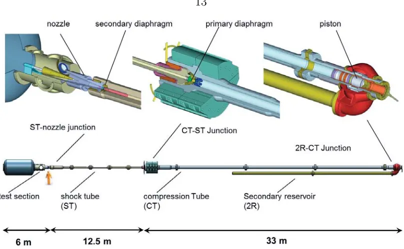
The facility used for all experiments in the present study is the T5 Hypervelocity Reﬂected Shock Tunnel located at the Graduate Aerospace Laboratories of the Cali-fornia Institute of Technology; see Hornung(1992) and Hornung and Belanger(1990) for details on the design and operation of this facility, a rendering of which is presented in Figure2.1. For a good explanation of the basic principles underlying piston-driven reﬂected shock tunnels, see Section 16.2 in Tropea et al. (2007).

2.1.1

Overview

(40)

Figure 2.1: Rendering of the T5 Hypervelocity Shock Tunnel. (Based on drawings prepared by Bahram Valiferdowsi.)

Shock Tube

Secondary Diaphragm

Nozzle _{Test Section}

Model Compression

Tube

Primary Diaphragm Piston

[image:40.612.123.527.57.306.2]

2R

Figure 2.2: Simpliﬁed schematic diagram of the T5 Hypervelocity Shock Tunnel. The section labeled “2R” is the secondary reservoir. See also Figure 2.5.

At the beginning of the experiment, the shock tube is ﬁlled with the desired test gas; in the present experiments, this is always N2, air, CO2, or a mixture of CO2 and

air premixed in the tank described and pictured in Section 2.1.2. The compression tube is ﬁlled sequentially with a mixture of He and Ar, and the secondary reservoir is ﬁlled with pressurized atmospheric air from the external holding tanks.

(41)

primary diaphragm is reached, it fails quasi-instantaneously and a strong shock wave is created at the contact surface between high-pressure driver gas and lower-pressure test gas in the shock tube. This shock wave propagates through the shock tube, accelerating, compressing, and heating the test gas, and is reflected off the end wall, simultaneously vaporizing the Mylar secondary diaphragm. The reflected shock wave propagates back through the already-shocked gas, further compressing and heating it, and also bringing it to rest. This stagnant, high-temperature, high-pressure slug of test gas serves as the reservoir for a contoured 100:1 area ratio converging-diverging nozzle, which accelerates the test gas to hypervelocity before it flows over the model. Chapter 3 provides a further description of the test article and its instrumentation, and Section 2.5 presents analysis of the uncertainty in flow conditions at the end of the nozzle and over the test article.

2.1.2

Gas Premixing Tank

To ensure complete mixture in the shock tube for air and CO2 mixture experiments,

(42)

[image:42.612.161.488.120.366.2]

76 L, and fill pressures for most cases are rarely higher than 100 kPa, this quantity of premixed gas is usually sufficient for at least five experiments.

Figure 2.3: Gas premixing tank.

In the present series of tests, the mixing tank was ﬁlled sequentially to the desired partial pressure of each gas several hours prior to any experiments. To ensure complete mixing and a uniform distribution of gas species, two 120 mm 12 VDC brushless computer fans were installed in the mixing tank and are run continuously prior to the experiment. These fans, pictured in Figure 2.4, are wired in parallel to an external transformer through a switch located on the mixing tank control panel.

For safety, a CO2 alarm that triggers at 5000 ppm, meeting OSHA speciﬁcations,

(43)

Figure 2.4: Gas premixing tank internal fans.

2.1.3

Shock Tube Cleaning Procedure

At the conclusion of each experiment, care must be taken to thoroughly clean the shock tube, nozzle, and model, each of which is to a varying degree coated with soot and other small particles carried in the driver gas. This cleaning step is especially critical for work on laminar to turbulent transition, as particulates in the freestream can destabilize the boundary layer and can lead to early instability (Fedorov and Koslov,2011,Fedorov,2013), including intermittent broad-band density disturbances as described in Parziale (2013) and transition to turbulence.

Prior to shot 2703, the standard T5 cleaning procedure consisted of pulling a bundle of clean white towels through the length of the shock tube once or twice, and propelling a bucket covered in towels down the length of the compression tube test section. This procedure was eventually found to be insuﬃcient for performing repeat-able experiments, in that inconsistent stability and transition results were sometimes obtained, and clouds consisting of dark particulate contamination were sometimes observed in schlieren movies during the test time. Both of these results were more likely in the next experiment performed after a shot with CO2 present in the shock

(44)

tube, and secondarily in the compression tube near its junction with the shock tube. We also determined that the most important segment of the tunnel to clean was the end of the shock tube immediately before the nozzle, where the “slug” of reservoir gas resides.

The cleaning procedure stabilized by shot 2760, and consists of the following steps: first, the final 2 m of the compression tube is dry polished with a wire wheel mounted on an electric drill, prior to propelling the towel-covered bucket through the length of the compression tube. Next, using an appropriate ventilator, gloves, and goggles, the final 2.1 m of the shock tube is polished with a wire wheel around which is wrapped a fresh 3M ScotchBrite Ultra-Fine Hand Pad (#7448) moistened with acetone, with additional acetone sprayed directly into the end of the tube. Over several polishing cycles, black, soot-laden solvent flows out of the end of the shock tube and is collected in a towel placed under the mouth. Next, a fresh towel is wrapped around a mop mounted at the end of a length of 1 in diameter aluminum conduit pipe, with a total pole length of 4 m. This towel is sprayed with acetone and, while twisting the pole, pushed into and then pulled out of the final 4 m of the shock tube. This is repeated at least eight times, inverting each towel once and then replacing it so that a clean surface is always exposed, until the towels return clean. Next, a bundle of several towels is rolled, sprayed with acetone, and pulled with a rope down the length of the shock tube from the nozzle end to the primary diaphragm end (so that any debris is drawn further away from the already cleaned test gas stagnation region). This process is repeated with fresh towel surfaces until the towels come through the tunnel clean, which usually takes at least 20 cycles. Finally, clean towels sprayed with denatured ethyl alcohol are pulled through the shock tube twice in the same manner in an effort to remove any acetone residue, and a single, balled dry towel is pulled through with a shop vacuum.

(45)

of ∼3 man-hours per experiment was devoted to cleaning), the primary diaphragm holder is cleaned with acetone and denatured ethyl alcohol. The test article, throat, and nozzle also accumulate dark soot-like dust, although not to the same degree as the shock tube, and are cleaned with Kimwipes sprayed with denatured ethyl alcohol.

Rather than using standard “Industrial”-quality gas bottles to ﬁll the shock tube, as had been the previous practice, reduced-contaminant “Breathing Air” was used from shot 2739. Finally, only Air Liquide “ALPHAGAZ” research-quality gas bottles were used from shot 2757, for all gas types. In this line of gas bottles, the supplier speciﬁes tight tolerances on the O2 vs. N2 partial pressure (±0.5%) for air, and

to-tal hydrocarbon contamination is less than 0.05 ppm. All of these measures, taken together, were successful in mitigating the eﬀects of particulate contamination and resulted in more consistent, clean, repeatable transition measurements. It is recom-mended that these cleaning and contaminant minimization measures be maintained for all future T5 experiments where ﬂow purity, optical measurements, and avoiding particulate contamination are important.

2.2

Measured Tunnel Quantities

P

_ST3

P

_res

P

_burst

P

ST4

2R Compression

Tube Shock Tube

Test Section Nozzle

Piston

Figure 2.5: Simpliﬁed schematic diagram of the T5 Hypervelocity Shock Tunnel with labeled pressure transducers at the diaphragm burst location, stations 3 and 4 (located 4.8 m and 2.4 m, respectively, from the end of the shock tube), and at the shock tube reservoir. See also Figure 2.2.

(46)

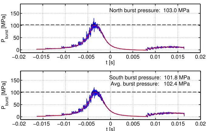
trans-ducers mounted at the primary diaphragm station. See Figure 2.5 for the transducer location and Figure 2.6 for an example of the burst pressure traces with the burst pressure level indicated. Together with the known shock tube ﬁll pressureP1, and the

composition of the driver gas and test gas, this measurement deﬁnes the diaphragm pressure ratio. Taking gas 1 as the unshocked test gas and gas 4 as the high-pressure (Pburst) driver gas, as is common in the literature, we can write (e.g., as inThompson

(1972)) the perfect gas relationship:

P4

P1

= 2γ1M

2

s −(γ1−1)

γ1+ 1

1− γ4−1 γ1+ 1

c1

c4

Ms−

1 Ms

−2γ₄ γ₄−1

(2.1)

This equation may be solved for the shock Mach number Ms at a given diaphragm

pressure ratio, and converted to shock speed Us using the known properties of gas 1.

Real gas properties and numerical methods can be used as discussed inBrowne et al.

(2008) to compute Ms without making the perfect gas assumption. In practice Ms is

calculated from the measured Us and Equation (2.1) is used to check the consistency

of the data.

The primary shock speed is measured experimentally by two time of arrival pres-sure transducers, at shock tube stations 3 and 4, mounted 2.402 m apart near the end of the shock tube. See Figure 2.5 for the transducer locations and Figure 2.7 for an example of the time of arrival pressure transducer traces with incident and reﬂected shocks marked.

The calculated value from Equation (2.1) is representative of the initial shock speed after the diaphragm bursts. The shock slows as it propagates through the shock tube and the boundary layer grows inside the tube. Hornung and Belanger

(47)

−0.02 −0.015 −0.01 −0.005 0 0.005 0.01 0.015 0.02 0

50 100 150

t [s] P burst

[MPa]

North burst pressure: 103.0 MPa

−0.02 −0.015 −0.01 −0.005 0 0.005 0.01 0.015 0.02

0 50 100 150

t [s] P burst

[MPa]

[image:47.612.154.495.69.285.2]

South burst pressure: 101.8 MPa Avg. burst pressure: 102.4 MPa

Figure 2.6: Raw (blue) and smoothed (red) pressure traces from the north and south burst pressure transducers for shot 2742, mounted in the primary diaphragm holder at the end of the compression tube (see Figure2.5). The peak value of the smoothed signal is marked with a dashed line.

−8 −6 −4 −2 0 2 4 6 8

0 20 40 60

t [ms]

P station #3 [MPa]

−8 −6 −5 −2 0 2 4 5 8

0 50 100

t [ms]

P station #4 [MPa]

Primary shock speed: 3017.6 m/s Reflected shock speed: 1482.7 m/s

Figure 2.7: Pressure traces from pressure transducers mounted at stations 3 and 4 on the shock tube (see Figure 2.5) for shot 2742, showing time of arrival signals at each station, from which are calculated the primary and reﬂected shock speeds at the end of the shock tube.

[image:47.612.147.504.374.584.2]

(48)

2 during past experiments in T5 with air (Hornung, 1991).

2.3

Reservoir Condition Calculation

The reservoir pressure, Pres, is directly measured by two pressure transducers mounted

at the shock tube end wall, immediately upstream of the nozzle throat. See Figure2.5

for the transducer locations and Figure 2.8 for an example of the reservoir pressure transducer traces with the period of relatively steady constant pressure supply to the nozzle conservatively indicated. This indicated period corresponds to the temporal extent of the experiment (allowing an additional period,∼0.3 ms, to account for the gas ﬂow time through the nozzle from the throat to the tip of the test article) and is selected individually from the reservoir pressure plot for each experiment. While Pres remains relatively constant for several milliseconds for some conditions in the

present study, the work of Sudani and Hornung (1998) indicates that the useful test time for the present enthalpy range is limited to ∼1 ms due to driver gas contamina-tion. As Sudani et al. (2000) recommend, undertailored (discussed subsequently in Section 3.2.1) conditions are used to minimize contamination.

The measured incident shock speed, Us, from Section 2.2 and the shock tube ﬁll

pressure P1 are used with the reflected eq routine from the Cantera (Goodwin,

2003;Goodwin,2009) Shock and Detonation Toolbox (Browne et al.,2008) with CO2

reaction rates taken from Smith et al. (1999) to calculate the equilibrium thermody-namic state of the gas after processing by the incident and reflected shock. The test gas is then isentropically expanded from the computed reservoir pressure state to the measured Pres from the transducers, which adjusts for the effects of wave reflections

(49)

−2 −1 0 1 2 3 4 5 6 7 8 0

20 40 60 80

t [ms] P res

[MPa]

P

res North: 53.6 MPa

−2 −1 0 1 2 3 4 5 6 7 8

0 20 40 60 80

t [ms] P res

[MPa]

P

res South: 57.8 MPa

P

[image:49.612.145.503.77.305.2]

res Average: 55.7 MPa

Figure 2.8: Raw (blue) and smoothed (red) pressure traces from the north and south reservoir pressure transducers for shot 2742, mounted at the shock tube end wall just upstream of the nozzle throat (see Figure 2.5). The steady test time, here about 0.9 ms long, is highlighted with dashed lines. This example is undertailored, as an expansion wave at the shock wave/contact surface interface is seen to lower the reservoir pressure prior to the useful test time (Tropea et al., 2007).

2.4

Nozzle Flow Calculation

2.4.1

1-D Nozzle Calculation

(50)

-displacement, deﬁned by the physical nozzle geometry A(x):

dU dx =

1 η

˙ σ−U

A dA dx dP

dx = − ρU

η

˙ σ− U

A dA

dx dρ

dx = ρ U η

˙

σ−M2U A

dA dx dy_i

dx =

W_iω˙_i ρU

The thermicity, ˙σ, is deﬁned as:

˙ σ ≡ k i=1 W W_i −

h_i C_pT

Udyi dx

The production rate, molar mass, mole fraction, and mass fraction of species i are, respectively, ˙ω_i, W_i, χ_i, and y_i. η≡(1−M2) is the sonic parameter.

The solution to these four coupled diﬀerential equations is implemented, for con-venience and backwards compatibility, with a similar nozzle format as that used by NENZF (Lordi et al., 1966), the previous nozzle ﬂow solver. Beierholm et al.

(2008) developed non-Cantera _Matlab subroutines that interface with the Cantera package to solve for nozzle ﬂow equations, including oneDflow, areafun,

non-ideal eq soundspeed, nonideal soundspeed, and isenfun. Coupled with

Cantera routines for computing net production rates, species, entropy, and enthalpy, these _Matlab functions are implemented in a new nozzle ﬂow solver, which takes as its gas state inputs the reservoir conditions described in Section 2.3, and evolves a Cantera gas object down the length of the deﬁned nozzle geometry. The chemical kinetics models used are described in Smith et al.(1999) and Gupta et al. (1990).

(51)

Ap-pendix B. Dissociated species mass fractions “freeze” during nozzle expansion when the density and temperature become too low to sustain collisions frequent enough for recombination and vibrational energy transfer. This effect leaves a greater fraction of dissociated, vibrationally excited species present in the mean flow than would be the case for equilibrium flows, or the comparable free flight conditions (Stalker, 1989).

2.4.2

Axisymmetric Nozzle Flow Simulations

In order to obtain more accurate values for the ﬂow properties over the test cone than are possible with the simple one-dimensional calculation described in Section 2.4.1, including a more accurate accounting of vibrational nonequilibrium, we begin with the same reservoir conditions computed with the procedure described in Section 2.3

and tabulated in Appendix A. Gas at each reservoir condition is computationally expanded through the nozzle using the CFD solver described below, rather than the one-dimensional calculation previously used in T5 studies, which is described inLordi et al. (1966).

(52)

noz-zle ﬂow is calculated on a single-block, structured grid with dimensions 492 cells by 219 cells in the streamwise and wall-normal directions, respectively (see Figure 2.9). The grid, used originally by Wagnild (2012), is clustered near the nozzle wall in order to suﬃciently resolve the boundary layer for both laminar and turbulent cases.

This nozzle computation is performed for every experiment in the present study, and provides the input conditions for the boundary layer calculations described in Section 4.1.2. For most of the current computational analyses, it is assumed that the boundary layer on the nozzle walls becomes turbulent in the reservoir and remains in this state for the remainder of the nozzle, but the eﬀect of a potentially laminar boundary layer on the nozzle wall on nozzle conditions is one of the variables examined in Section 2.6. In all cases the wall temperature for the nozzle is taken to be 297 K.

−100 0 100 200 300 400 500 600 700 800 900

0 50 100 150

[m]

Figure 2.9: Axisymmetric grid of 492 cells by 219 cells in the streamwise and wall-normal directions, respectively, used for nozzle ﬂow computations.

2.5

Run Conditions and Uncertainty Estimates

2.5.1

Overview

The shock speed is measured by two time of arrival pressure transducers with a known physical displacement along the axial direction of the shock tube, as discussed in Section 2.2. These transducers have an approximate measurement uncertainty of 8×10−6 _{s. The uncertainty in the shock speed measurement thus increases as}

(53)

present study, the uncertainty is ∼30 m/s. The shock tube ﬁll pressure uncertainty is ∼0.25 kPa, and the measured reservoir pressure uncertainty, based upon recorded pressure traces such as those presented in Figure 2.8, is typically ∼4 MPa. The measured uncertainties are presented in Table 2.1.

Uncertainties on the calculated quantities are estimated by perturbing Cantera Shock and Detonation Toolbox condition computations, similar to those described in Section 2.3, within the range of the uncertainties on the measured shock speed, reservoir pressure, and initial shock tube pressure. Only experiments with measured shock speeds that fall within the uncertainty for the adjusted shock speed curve1

predicted by the shock jump conditions from the primary diaphragm burst pressure, driver gas composition, and initial shock tube conditions are included in the present data set.

There are a number of other potential sources of measurement error, including nonideal gas behavior in the reservoir due to the high pressure, the extrapolation of the shock speed (which decays as it propagates down the shock tube) to the end wall, nonuniformity of reservoir conditions due to nonideal shock reflection, and the method of correcting flow conditions from the ideal reflected-shock pressure to measured reser-voir pressure using an isentropic expansion. Furthermore, the one-dimensional con-toured nozzle computation, described in Section 2.4.1, does not account for bound-ary layer growth within the nozzle, off-design operation conditions that lead to flow nonuniformity, or vibration-translation nonequilibrium and freezing within the noz-zle, which is particularly significant for the N2 cases. However, the axisymmetric

nozzle computations described in Section 2.4.2, which provide the input conditions for boundary layer analysis, do include these nozzle eﬀects.

Run conditions and uncertainty estimates for three typical T5 conditions taken from low enthalpy (2649), mid-range enthalpy (2645), and high enthalpy (2788) shots

(54)

Measurement Symbol Uncertainty Units

Shock Speed Us ±13–53 m/s

Shock Tube Fill Pressure P1 ±0.25 kPa

Reservoir Pressure Pres ±2–4 MPa

Table 2.1: Estimated uncertainty of measured quantities, all shots.

are made below. Computed boundary layer edge condition uncertainties are estimated at the edge of the cone boundary layer using a Taylor-Maccoll solution from the nozzle exit conditions.

The ﬂuid properties of greatest interest in the present work are typically those near the surface of the conical test article, after the conical shock at the boundary layer edge (see Tables 2.4, 2.7, and 2.10), since those quantities deﬁne the boundary layer’s properties. For typical conditions from a wide range of enthalpies, the greatest uncertainty at the boundary layer edge in percentage terms is found to be the edge pressure. This is a result of the relatively uncertain measurement of reservoir condi-tions at the end of the shock tube. The smallest uncertainty is found in the Mach number and edge velocity.

2.5.2

Uncertainty Estimates (Low Enthalpy, Shot 2649)

Experiment 2649 had a computed enthalpy of 4.78 MJ/kg. Uncertainty values for the measured tunnel quantities, computed thermal quantities, and computed boundary layer edge quantities are presented in Tables 2.2,2.3, and2.4, respectively.

Measurement Symbol Value Uncertainty Units Percent

Shock Speed Us 2256 ±17 m/s 0.8

Shock Tube Fill Pressure P1 90.0 ±0.25 kPa 0.3

Reservoir Pressure Pres 22.2 ±2 MPa 9.1

(55)

Computed Quantity Symbol Value Uncertainty Units Percent

Reservoir Enthalpy hres 4.78 ±0.14 MJ/kg 3.0

Reservoir Temperature Tres 3785 ±78 K 2.0

Reservoir Density ρres 20.1 ±1.5 kg/m3 7.4

Freestream Temperature T_∞ 604 ±23 K 3.8

Freestream Density ρ_∞ 0.0438 ±0.0066 kg/m3 8.5

Freestream Pressure P_∞ 7.63 ±1.7 kPa 11.3