2017 International Conference on Computer Science and Application Engineering (CSAE 2017) ISBN: 978-1-60595-505-6
An Algorithm for Computing a Hamiltonian Cycle
of Given Points in a Polygonal Region
Yiyang Jia and Bo Jiang*
School of Information Science and Technology, Dalian Maritime University, Dalian, China
ABSTRACT
In this paper, for a point set X in a simple polygon P, we present an algorithm to
compute a Hamiltonian cycle which avoids the boundary of P and accesses all points of
X. Computing a Hamiltonian cycle of given points in a simple polygon is a novel transformation of the general Hamiltonian problems and the problem of finding simple paths on given obstacles in a simple polygon. In our solution, we first construct the geodesic convex hull G of X inside P, and then find simple paths turn only at the points of X for two adjacent vertices in X along the boundary of G which are invisible to each other. After an original Hamiltonian cycle is found, we insert the remaining points to it. Finally, we present an O((n2+m)nlogm) time algorithm (n is the number of points in X
and m is the number of P’s vertices) to report a Hamiltonian cycle if it exists or report
that no such cycle exists.
INTRODUCTION Background
Computing a Hamiltonian cycle of given points in a simple polygon is an open problem posed by Cheng Q. et al., as a transformation of finding simple paths among obstacles in a simple polygon [1]. The problem can be described as follows: Suppose that there is a set X of n given points in a simple polygon P in the plane, the objective is to construct a Hamiltonian cycle HX (without self-intersections) which accesses all
points in X and avoids the boundary of P, so that each edge of HX does not intersect with
the boundary of P (except for the vertices of P). If such HX exists, output it, otherwise
report that no such cycle exists. When P is convex, HX certainly exists and can simply
be found in O(nlogn) time by using the method provided in [1].
Over the past two hundred years, many researchers have studied the related problems of Hamiltonian cycle or path. Although the original Hamiltonian path problem is proven to be an NPC problem [2], the time complexity of finding Hamiltonian cycles can be reduced to polynomial time under certain conditions, such as finding Hamiltonian cycles in distance-hereditary graphs [3], or in co-comparability graphs [4], or in semi-complete multipartite digraphs [5], and so on.
In our work, the objective is actually finding a Hamiltonian cycle without self-intersections in part of a complete graph limited in a given polygon region. We use a method which consists of two parts: the first part is constructing the geodesic convex hull of the given points and finding the simple paths between a pair of adjacent invisible points, which can obtain an initial Hamiltonian cycle; the second part is inserting the remaining points to the initial Hamiltonian cycle.
For computing the geodesic convex hull, G. Toussaint first proposed an O(k) time
algorithm for computing the geodesic convex hull inside a simple polygon (k is the total
number of vertices of the given polygon region and the given points) [10], and this method was improved by Wiederhold P. and Reyes H. in [11].
For computing the simple paths, Tan X. and Jiang B. present an O((n2 + m)logm)
time algorithm for computing simple paths on given points in a polygonal region or
reporting no such path exists(n is the number of given points and m is the number of
vertices of the given polygonal region) [12].
Our Work
We show in the following sections that if P is a simple polygon and X is the given
point set in P, the problem of computing a Hamiltonian cycle of X in P can be solved in
O((n2+m)nlogm) time (n is the number of points in X and m is the number of P’s
vertices). We then present a universal algorithm to compute a Hamiltonian cycle of X in
P or report that no such cycle exists to solve the open problem posed in [1].
The novelty of our algorithm is its simplicity: instead of considering the relationship between edges and points in a planar graph, our algorithm uses only the known algorithms for computing simple paths and the geodesic convex hull, as well as simple methods for inserting remaining points to the initial Hamiltonian cycle. Besides, our solution sheds more light on the problem of developing a polynomial-time solution to the open problem of computing the simple Hamiltonian path from a start point to an end point which avoids the boundary of the region and accesses all given points [12].
PRELIMINARIES AND NOTATION
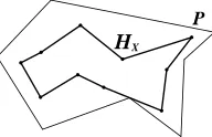
Let P denote the input simple polygon with m vertices, and X denote the given point set with n points in P, X={ x1, x2, …, xn }. Our objective is to find a Hamiltonian cycle
denoted by HX (without self-intersections) which accesses all the points in X and turn
only at the points of X, and does not intersect with the boundary of P (except for the
vertices of P), as in Figure 1. In the following sections, without loss of generality, we
assume that P is a concave polygon, otherwise HX can be found in O(nlogn) time [1].
P
[image:2.612.249.345.607.669.2]HX
Let G denote the geodesic convex hull of X inside P which is obtained by allocating a tight thread around X but within P (the vertices of P can be included on the boundary of G), HG denote its boundary, XG denote the pointsin X accessed by HG. A path is
simple if it is non-self-intersecting. Two points s, t in P are said to be visible to each
other if the line segment connecting them (denoted byst) is entirely contained in P,
otherwise they are said to be invisible.
For s, t in P which are invisible to each other, if there exists a polygonal simple path
p between s and t which turns only at the points in X and avoids going across the boundary of P, then we call p a (s, X, t)-path.
In our approach, H0 is defined as an initial Hamiltonian cycle without
self-intersections which accesses only some of the points in X. H0 is obtained by finding
simple paths between an adjacent pair of invisible points in X along HG. The points in X
outside H0 are denoted by X1.
CONSTRUCTION OF HX
Construction of H0
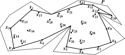
We first construct the geodesic convex hull G of X inside P with Algorithm of Determining the Relative Convex Hull for Simple Polygons in the Plane given in [11] which can be done in O(m+n) time, e.g. the geodesic convex hull G of the given points in Figure 2 is denoted by black solid segments inside P, where XG={x1, x2, …, x12}.
x28
x27
x26
x25
x24
x23
x22
x21
x20
x19
x18
x17
x16
x15
x14
x13
x12
x11
x10
x9
x8
x7
x6
x5
x4
x3
x2
x1
[image:3.612.192.403.380.474.2]P
Figure 2. The geodesic convex hull G of X in P.
Then, with an arbitrary pair of points {xj, xk} in X which are adjacent in the
clockwise(or counterclockwise) order on HG and are invisible to each other, HG can be
divided into two paths in a same direction, one is from xj to xk, the other one is from xk to
xj. For convenience, we denote the point sequences respectively accessed by them in the
clockwise order as sjk and skj. For instance, for {x5, x4} in Figure 2, sjk={x5, x4}, skj={x4,
x3, x2, x1, x12, x11, x10, x9, x8, x7, x6, x5}
We use the method given in [12] to find two simple paths between xj and xk on X.
The first one denoted by p1 has to contain all points in skj by the same order; the second
x28
x27
x26
x25
x24
x23
x22
x21
x20
x19
x18
x17
x16
x15
x14
x13
x12 x 11
x10
x9
x8
x7
x6
x5
x4
x3
x2
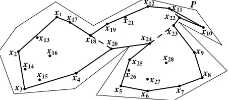
[image:4.612.187.406.57.157.2]x1 P
Figure 3. H0 of X in Figure 2.
H0 is obtained by a combination of p1 and p2.
For instance, H0 of the given points in Figure 2 is shown in Figure 3, in which p1
accesses x4, x3, x2, x1, x18, x12, x11, x10, x22, x23, x9, x8, x7, x6, x5 by order and p2 accesses x5,
x24, x20, x4 by order.
If H0 does not exist, then report that HX does not exist, an example is given below
(See in Figure 4).
x15
x14
x13
P x1
x2
x3
x4
x5 x6 x7
x8
x9
x10
x11
x12
Figure 4. Example of the situation that H0 does not exist.
Lemma 1. The necessary condition for the existence of HX is that H0 exists.
Proof. Since H0 does not exist iff: (1) p1 does not exist; or (2) p2 does not exist. For
(1), it means that no simple path inside G (on the point set X-XG) is between a pair of
invisible points (denoted by xj, xk) in the clockwise order on HG , so we cannot find a HX
on which xj and xk can be connected in the clockwise order without self-intersection
because if xj and xk are connected by some points (e.g. xi) in XG on HX, then the sub-path
between xj and xk must intersects with the sub-path between xi’s adjacent two points on H0; for (2), it is clear that we cannot find a HX without self-intersection. Therefore
Lemma 1 is proven.
In fact, the existence of H0 is also the sufficient condition of the existence of HX, this
point will be described in detail in the following sections.
Lemma 2. It takes up to O((n2 + m)nlogm) time to compute H0 or report that HX
does not exist.
Proof. Since p1 has to contain all points in skj by the same order, and there are at
most n points in skj, so we can find p1 in O((n2 + m)nlogm) time or report that it does not
exist by using the method given in [12]. Also, since p2 has to make no intersection with
p1, so we can find p2 in O((n2 + m)nlogm) time or report that it does not exists by using
the method given in [12]. H0 is obtained by a combination of p1 and p2, therefore we can
get H0 or report that H0 does not exist in O((n2 + m)nlogm) time. According to Lemma 1,
we can report that HX does not exist in O((n2 + m)nlogm) time.
[image:4.612.194.399.290.386.2]Handling the Points in X1
After H0 is obtained, we handle the points in X1, which are excluded from the
internal area surrounded by H0 due to the simple paths between pairs of adjacent
invisible points on HG. We insert these outside points into the corresponding simple
paths with the Graham Scanning Algorithm [13] so that we can obtain a Hamiltonian cycle that each of the given points is either on it or inside the area surrounded by it. The specific strategy is:
For each concave vertex pi on HG between two adjacent points xa, xb which are
invisible in the clockwise order on HG, connect pi with the concave vertices on H0
between xa, xb so that X1 is divided into subsets limited by the regions surrounded by
connecting segments, H0 and HG. Then, use the points in these subsets to form convex
chains but avoid right-turns. Finally replace the corresponding parts on H0 by these
convex chains. For points on same connecting segments, they can be considered as in either region adjacent to the connecting segment, but they should be computed only once.
For instance, for Figure 3, x17 should be inserted between x1 and x18; x19 and x21
should be inserted between x18 and x12; x25 and x26 should be inserted between x5 and x24.
But when constructing the convex chain, since x19, x21, x12 and x5, x26, x25 form right
turns, thus x21 and x25 are removed from the convex chains, and the final result is as in
[image:5.612.185.408.350.449.2]Figure 5. x28 x27 x26 x25 x24 x23 x22 x21 x20 x19 x18 x17 x16 x15 x14 x13 x12 x11 x10 x9 x8 x7 x6 x5 x4 x3 x2 x1 P
Figure 5. Example of handlingX1 in Figure 3.
Handling the Internal Points
For the Hamiltonian cycle obtained after the points in X1 are handled, we first divide
its internal region into convex regions based on a convex decomposition method in [14] which costs O(n) time.
For instance, we can divide the internal of the Hamiltonian cycle in Figure 5 into several regions as in Figure 6.
x28 x27 x26 x25 x24 x23 x22 x21 x20 x19 x18 x17 x16 x15 x14 x13 x12 x11 x10 x9 x8 x7 x6 x5 x4 x3 x2 x1 P
[image:5.612.185.411.588.687.2]For each convex polygonal region obtained by the convex decomposition, insert its internal points into an arbitrary edge of this region which is also an edge of the Hamiltonian cycle obtained after the points in X1 are handled. The specific strategy is as
follows:
Suppose a point set A is inside the convex region where an edge xpxq is located,
the method of inserting the points in A into the Hamiltonian cycle is: (1) Connect xp with each point in A;
(2) Sort the points in A according to the slope of the connecting line segments in (1), for points with the same slope, sort them according to the length of the connected line
segments (from short to long), a sequence S can be obtained;
(3) Insert xp before the first element in S, xq after the last element in S, a polygonal
chain can be obtained by connecting all the points in S by order, and replace xpxq by
the new chain.
Since each obtained polygonal chain has following properties:
(1) It does not intersect with the boundary of its own region except for the endpoints of the replaced boundary segment since all of its points are the internal points of the region except for the endpoints of the replaced boundary segment;
(2) It does not intersect with the connecting segments in other regions or the boundary of other regions since it is inside a fixed region;
(3) It is constructed in an order which makes it has no self-intersection on itself.
Therefore, using the above method, we can get HX without self-intersections. For
instance, we deal with the internal points in Figure 6, replace x20x4 by using the
polygonal chain of the sequence {x20, x13, x16, x14, x15, x4}, and replace x24x20 by using
the polygonal chain of the sequence {x24, x21, x20}, and replace x25x24 by using the
polygonal chain of the sequence {x25, x26, x27, x28, x24}, then we get HX of the given
points in Figure 2, see in Figure 7.
x28
x27
x26
x25
x24 x23
x22
x21
x20
x19
x18
x17
x16
x15
x14
x13
x12
x11
x10
x9
x8
x7
x6
x5
x4
x3
x2
[image:6.612.190.406.465.571.2]x1 P
Figure 7. HX of X in Figure 2.
Now, we give an algorithm, named HCPP (a Hamiltonian Cycle of the given Points in a Polygon), for computing HX as follows.
Algorithm HCPP:
Input: A set of points X and the vertices of a simple polygon P. Output: A Hamiltonian cycle HX or report that HX does not exist.
1 Construct the geodesic convex hull G of X inside P
2 Construct H0:
2.1 Denote the point sequences accessed by xj and xk as sjk and skj.
2.2 Find two simple paths between xj and xk on X: p1(contains all points in skj by the same order), p2(makes no intersection with p1).
2.3 Construct H0 by a combination of p1 and p2.
3 Handle the points in X1 outside H0:
For each concave vertex pi on HG between two adjacent invisible points(xa, xb):
3.1 Divide X1 by connecting pi with the concave vertices on H0 between xa, xb;
3.2 Use the points in these subsets to form convex chains but avoid right-turns;
3.3 Replace the corresponding parts on H0 by these convex chains.
4 Handle the internal points to construct HX:
4.1 Decompose the internal region into convex regions;
For each convex polygonal region contains a point set (A) and an edge(xpxq ):
4.2 Connect xp with each point in A;
4.3 Sort the points in A according to the slope of the connecting line segments to get a sequence S;
4.4 Replace xpxq by a polygonal chain of S.
For the algorithm above, we have Theorem 1.
Theorem 1. Algorithm HCPP can be done in O((n2+m)nlogm) time.
Proof. Constructing G costs O(n+m) time by using the method of computing the geodesic convex hull inside a simple polygon proposed by G. Toussaint in [10]. And we have already proved in Lemma 2 that constructing H0 or reporting that HX does not exist
costs O((n2+m)nlogm) time. If HX exists, it takes O(nlogn) time further to handle the
points in X1 by using the Graham Scanning Algorithm proposed in [13], and O(n) time
to handle the internal points by using the convex decomposition method proposed in [14] and a method of inserting the remaining points into the path one by one in order. Therefore, the total time complexity of algorithm HCPP is O((n2+m)nlogm). Theorem 1 is hold.
CONCLUSIONS
In this paper, we present an algorithm to compute a Hamiltonian cycle of given points in a polygonal region, which takes O((n2+m)nlogm) time to compute a
Hamiltonian cycle of a point set X in a simple polygon P which avoids the boundary of
P and accesses all points of X or report no such cycle exists. Whether a more efficient
algorithm can be developed to solve this problem is open.
Our method can be further used to find a polynomial-time solution to the open problem of computing the simple Hamiltonian path from a start point to an end point which avoids the boundary of the region and accesses all given points [1], we are now working on this direction.
ACKNOWLEDGEMENT
REFERENCES
1. Cheng, Q., Chrobak, M., and Sundaram, G. 2000. “Computing simple paths among obstacles,”
Comput. Geom., 16: 223-233.
2. Michael R. Garey and David S. Johnson. 1979. “Computers and Intractability: A Guide to the Theory of NP-Completeness,” W.H. Freeman, ISBN 0-7167-1045-5 A1.3:GT37–39, pp. 199-200.
3. R.W. Hung and M.S. Chang. 2005. “Linear-time algorithms for the Hamiltonian problems on dis-tance-hereditary graphs,” Theoretical Computer Science, 341, pp. 411-440.
4. J.S. Deogun and G. Steiner. 1994. “Polynomial algorithm for Hamiltonian cycle in co-comparability graphs,” SIAM Journal on Computing, 23: 520-552.
5. J. Bang-Jensen, G. Gutin, and A. Yeo. 1998. “A polynomial algorithm for the Hamiltonian cycle problem in semicomplete multipartite digraphs,” Journal of Graph Theory, 29: 111-132.
6. Frank Rubin. 1974. “A search procedure for Hamilton paths and circuits,” J. ACM, 21(4): 576-580. 7. William Kocay. 1992. “An extension of the multi-path algorithm for finding Hamilton cycles,”
Discrete Mathematics, 101(1-3):171-188.
8. A. Chalaturnyk. 2008. “A Fast Algorithm for Finding Hamilton Cycles,” M.Sc. Thesis at the University of Manitoba, Manitoba.
9. Blazewicz J, Kasprzak M. 2012. “Reduced-by-matching Graphs: Toward Simplifying Hamiltonian Circuit Problem,” Fundamenta Informaticae, 118(3): 225-244.
10. Toussaint, G.T. 1989. “Computing geodesic properties inside a simple polygon,” Invited paper, Special Issue on Geometric Reasoning, Revue D’Intelligence Artificielle, 3(2): 9-42.
11. Wiederhold, Petra, and H. Reyes. 2015. "Relative Convex Hull Determination from Convex Hulls in the Plane," International Workshop on Combinatorial Image Analysis Springer, Cham, pp. 46-60. 12. Tan, Xuehou, and B. Jiang. 2014. “Finding Simple Paths on Given Points in a Polygonal Region,”
International Workshop on Frontiers in Algorithmics Springer International Publishing, pp. 229-239.
13. RL Graham. 1972. “An efficient algorithm for determining the convex hull of a finite planar set,”
In-formation Processing Letters, 1(4): 132-133.