Posterior Constraint Selection for Nonnegative Linear Programming

http://www.scirp.org/journal/ajor ISSN Online: 2160-8849

ISSN Print: 2160-8830

Posterior Constraint Selection for Nonnegative

Linear Programming

H. W. Corley*, Alireza Noroziroshan, Jay M. Rosenberger

Center on Stochastic Modeling, Optimization, & Statistics (COSMOS), The University of Texas at Arlington, Arlington, TX, USA

Abstract

Posterior constraint optimal selection techniques (COSTs) are developed for nonnegative linear programming problems (NNLPs), and a geometric inter-pretation is provided. The posterior approach is used in both a dynamic and non-dynamic active-set framework. The computational performance of these methods is compared with the CPLEX standard linear programming algo-rithms, with two most-violated constraint approaches, and with previously developed COST algorithms for large-scale problems.

Keywords

Linear Programming, Nonnegative Linear Programming, Large-Scale Problems, Active Set Methods, Constraint Selection,

Posterior Method, COSTs

1. Introduction

1.1. The Nonnegative Linear Programming

Consider the linear programming (LP) problem

( )

_{P Maximize z=c x}T (1)

subject to

≤

Ax b (2)

0,

≥

x (3) where c _and x _{are n-dimensional column vectors of objective coefficients} and variables respectively; A is an m n× matrix   aij with 1×n row

vec-tors ai,i=1,, ;m b is an m×1 column vector; and 0 is an n×1 vector of

zeros.

The non-polynomial simplex methods and the polynomial interior-point bar-rier-function algorithms are currently the principal two-solution approaches for How to cite this paper: Corley, H.W.,

Noroziroshan, A. and Rosenberger, J.M. (2017) Posterior Constraint Selection for Nonnegative Linear Programming. Ameri-can Journal of Operations Research, 7, 26- 40.

http://dx.doi.org/10.4236/ajor.2017.71002

Received: November 17, 2016 Accepted: January 8, 2017 Published: January 11, 2017

Copyright © 2017 by authors and Scientific Research Publishing Inc. This work is licensed under the Creative Commons Attribution International License (CC BY 4.0).

solving problem P, but for either there are problem instances for which it performs poorly [1]. Since the principle use of LP in industrial applications is in binary and integer programming algorithms, however, pivoting algorithms with efficient post-optimality analysis are frequently preferable to interior-point me-thods. On the other hand, simplex methods often cannot solve large-scale LPs at a speed required by many current applications. The purpose here is to develop an approach for solving a certain class of LPs faster than existing methods.

In this paper we consider the nonnegative linear programming problem (NNLP), which is the special case of P with ai≥0 but ai≠0,i=1,, ;m

0

>

b ; and c>0. NNLPs model a large number of linear programming appli-cations such as determining an optimal driving path for navigation systems us-ing traffic data [2], updating flight status due to weather conditions [3], and de-tecting errors in DNA sequences [4]. NNLPs have the following two important properties:

1) the origin x 0= is feasible, 2)

1, , .

min i : 0 , 1, ,

j

j

i m

ij

b

x a j n

i a

=

 

≤ _ > _ =

 

 

Thus NNLPs have a bounded feasible region and bounded objective function if and only if no column of A is a zero vector. It follows that the boundedness of an NNLP objective function is easily verifiable without computation.

1.2. Background

We propose here an active-set method to solve nonnegative linear programming problems faster than current approaches. Our method divides the constraints of problem P into operative and inoperative constraints at each active-set

itera-tion. Operative constraints are those active in the current relaxed subproblem , 1, 2, ,

r

P r=  of P at iteration r, while the inoperative ones are constraints of the problem P not active in Pr. In our active-set method we iteratively solve P r_r

,

=1, 2,



, of P after adding one or more violated inoperative

con-straints from (2) to Pr−1until the solution *

r

x to P_r is a solution to P.

Active-set methods have been studied by Stone [5], Thompson et al. [6], Adler et al. [7], Zeleny [8], Myers and Shih [9], Curet [10], and Bixby et al. [11], among others. The term ‘‘constraint selection technique’’ was introduced in [9], while the approaches of [7] and [8] illustrate two distinct classes of active-set methods. When the constraint selection metric for choosing violated inoperative constraints to be added to Pr does not depend on the solution

*

r

x , the asso-ciated active-set method is called a prior method. On the other hand, if the con-straint selection at Pr does depend on

* r

x , it is called a posterior method. Ad-ler et al. [7] developed a prior method in which a violated inoperative constraint was chosen randomly at each active-set iteration. Zeleny [8] proposed a post-erior method in which the inoperative constraint most violated by *

r

cutting plane method of [13], and as part of the sifting algorithm of [11] for column generation.

More recently, Corley et al. [14] developed a geometric prior active-set me-thod for P called the cosine simplex method. At each active-set iteration r, a

single violated constraint maximizing the cosine of the angle between ai and c is added to the operative set for Pr. This cosine constraint selection

crite-rion is equivalent to the “most-obtuse-angle” pivot rule for the modified simplex algorithm introduced by Pan [15], where it was applied to the dual problem for P. Junior and Lins [16] also utilized a cosine criterion to choose an initial basis for the simplex algorithm on P resulting in a fewer number of simplex

itera-tions.

References [17] [18] [19] [20] are most directly related to the current work and involve the authors here. In [17], Corley and Rosenberger proposed the constraint selection metric maximizing

(

, ,

)

i i i

i

RAD a b c =a c_b (4)

for NNLPs. RAD is a geometric constraint selection criterion for determining the constraints most likely to be binding at optimality. In the associated ac-tive-set algorithm of [18], all constraints of (2) are initially ordered by decreasing value of RAD prior to solving an initial bounded problem P0 by the primal simplex. The dual simplex is then used when violated inoperative constraints are added according to their RAD value. In computational experiments, RAD proved superior to existing linear programming methods for NNLPs. A similar constraint selection metric GRAD was developed in [19] to solve general linear programs (LPs). Finally, in [20] a dynamic active-set method was developed for adding a varying number of violated constraints at Pr based on progress at

1.

r

P− It was incorporated into both RAD and GRAD to improve the computa-tional results of [18] and [19].

1.3. Overview

In this paper a posterior constraint selection metric NVRAD is developed for NNLPs. NVRAD may be considered as a posterior version of RAD. The post-erior NVRAD is then implemented in the dynamic framework of [20]. It should be noted that a constraint selection metric and the associated active-set method are identified by the same name- in this case NVRAD. For the active-set method NVRAD, we provide extensive computational extensive computational experi-ments to show that it solves NNLPs faster than other computational methods, including RAD and various versions of the existing posterior active-set method VIOL described above.

for NNLPs than all CPLEX solvers, as well as faster than VIOL and RAD. HYBR appears slightly faster than NVRAD. In Section 4, we present conclusions. Throughout the paper, both a constraint selection metric and the associated ac-tive-set algorithm are identified by the same name-RAD or NVRAD, for exam-ple. The use the term should be clear from context. The active-set algorithm it-self is called a COST, i.e., a “Constraint Optimal Selection Technique”.

2. NVRAD

2.1. Definition and Interpretation

Let *

r

x be the current optimal solution for some P_r with a perpendicular dis-

tance i *r i i

b

d=ax −

a to a violated hyperplane a xi =bi. It follows that * . r i i i i i d b b b − = ax

a

(5)

Note that i i

b

a is the perpendicular distance of hyperplane i i

b

=

a x to the

origin. Consequently, it follows that choosing a violated hyperplane a xi =bi with a maximum value i *r i

i

b b

−

x

a _{on the right side of (5) can be interpreted}

from the left side of (5) as selecting a violated constraint giving the deepest cut based on information derived from *

r

x . But from [18], the expression i i

b

a c on

the right side of (4) is the distance from the origin to the hyperplane a xi ≤bi along the vector c, i.e., the direction of steepest ascent for the objective

func-tion (1) of the NNLP P. For this reason, in [18] the inoperative constraint maximizing RAD

(

ai, ,bi c

)

is deemed the best constraint to add to Pr based

on prior information. We combine this prior information (4) with the posterior information on the right side of (5) by multiplying them to give

(

*

)

(

*

)

2

, , , i .

i i r i r i

i

c

NVRAD b b

b

=a −

a c x a x (6)

Equation (6) thus incorporates global information from RAD with local in-formation at *

r

x , and our posterior active-set method adds to Pr an

inopera-tive constraint _i* for which

(

*

)

*

*

2 OPERATIVE

arg max i i r i : i r i .

i _i

i b b

b

∉

 

 ₋ 

∈  > 

 

 

a c

a x a x (7)

We mention that the term 2

i

b in the denominator of (7) works better than

simply bi. This fact was established in computational results not reported here but obtained to support the above derivation.

2.2. The Dynamic Active-Set Algorithm

ap-proach is now used for NVRAD. Let *

r

x be the optimal extreme point for P_r,

with θr the angle between

*

r

x and c. Then

* T

* cos r ,

i r

θ = c x c

x (8)

is nonnegative since Pr is also an NNLP. We would like to decrease θr at each

active-set iteration so that *

r

x points more in the same direction as the gradient c of the objective function in (1). We adapt our dynamic heuristic of [20] that adds a varying number of violated inoperative constraints to Pr according to

the progress made Pr−1 in reducing the angle θr−1. As our ideal goal, let θ =r 0 in (8) to give

T * * .

r = r

c x x c (9)

When θ =r 0, it follows from (9) that

( )

* 2 1 * 1 2 1 . n

j rj n

j rj j n j j c x x c = = = =

∑

∑

∑

(10)

Letting ⋅ _{denote absolute value, define}

( )

_{* 1} *

( )

_* 2 1 2

1 n

j rj n

j

r r n j rj

j j c x x c δ = = = =

∑

−

∑

∑

x (11)

as a measure of the performance of our active-set method at iteration r. The value of

( )

*

r r

δ x decreases as θ_r decreases. Such a decrease usually occurs as *

r

x approaches an optimal extreme point of P itself.

The dynamic COST NVRAD for solving NNLPs is described as follows. Con-straints are initially ordered by the RAD constraint selection metric (4). To con-struct P0 we choose constraints from (2) in descending order of RAD (since there is no *

r

x ) until the A₀ matrix of has no 0 column, i.e., until each variable

j

x has an aij>0. These selected constraints become the constraints of P0, and we say that the variables are covered by the inequality constraints of the ini-tial problem. P0 is then solved by the primal simplex to achieve an initial solu-tion *

0,

x and δ₀

( )

x*₀ is calculated. At iteration r let γ_r be the number of constraints of problem P violated by x*r. Then at iteration r−1 and r, the

values of 1

( )

* 1

r r

δ − x− and δr

( )

x*r are calculated; and the percentage of

im-provement made in reducing the angle between vectors *

r

x and c at iteration r is measured by

( ) ( )

( )

* * 1 1 * 1 1

max 0, r r r 100, 1, 2, .

r r r r _r δ δ ω δ − − − −   ₋   _{ } = _{ }× =    _{ }    x x

x (12)

With

[ ]

⋅ _{denoting the greatest integer function, let}

(

)

(

1

)

1

1

1 ln , 1, 2, , if 1

, 1, 2, , if 1,

r r r r

r r r

r

r

ϕ ϕ ω ω

ϕ γ ω

− +

+



 _{= × +}  _{= >}

  = = ≤    

where ϕ =1 200. The value of ϕr is an upper bound on the possible number of violated constraints that can be added at active-set iteration r. The actual number added is min

{

ϕr+1,γr

}

. The active-set function ϕr increases at every iteration since the optimal value of the objective function for Pr is usually less

affected by a constraint with a small value of (6) than one with a large value. Hence, more violated constraints should be added as r _{increases. Equation} (13) represents one approach for doing so. If ωr> e (Euler’s number), for ex-ample, then ϕr+1=ϕr. If ω =r 1.01, then ϕr+1=101 .ϕr In other words, a much larger number and perhaps all of the remaining violated constraints could be added. NVRAD stops when γ =r 0, i.e., when there are no more violated constraints.

The pseudocode for dynamic NVRAD algorithm is as follows. Step 1—Identify constraints to initially bound the problem. 1: *

0, BOUNDING

← ← ∅

a 2: while *

0



a do

3: *

(

)

EXPLORED

arg max

Let , ,i i .

i

i RAD b

∉

∈ a c

4: _if * _{0 and} * _{0 then}

j ij

j a

∃ = >

a

5: BOUNDING←BOUNDING∪

{ }

i ? 6: end if

7: *

i

← +

* *

a a a

8. Optimized←false 9: end while

Step 2—Using the primal simplex method, obtain an optimal * 0

x for the ini-tial problem.

( )

0

T Maximize subject to , BOUNDING 0. i i P z b i = ≤ ∈ ≥ c x a x x

Step 3—Perform the following iterations until an answer to problem P is

found. 1: r←0

2: while Optimized = false do 3: Calculate

( )

*

.

r r

δ x

4:

( ) ( )

_{( )}

* *

1 1

*

1 1

if 1 then r max 0, r r r 100

r r

r

r ω δ δ

δ − −

− −

  ₋ 

 _{ }

> = _{ }×

 

 _{ }

 

x x

x

5:

(

(

)

1

)

1

ifωr 1 then ϕr ϕr 1 lnωr

− + = × + 

> _{ }

6: else if ω ≤r 1 then ϕr+1=γr

7: end if 8: else ϕ ←r 0 9: end if

10: *

, 1, , rows if a xi r >bi i=  then

11:

{

*

}

, 1, , ro

#{ i ws

r r b ii

12: *

(

*

)

(

*

)

* OPERATIVE

arg max , , ,

Let : .

2

i

i i r i r i i r i

i _i

b

i NVRAD b b

b

∉

 

 ₋ 

∈  = > 

 

 

a c

a c x a x a x

13: for i=1,,min

{

ϕr+1,γr

}

OPERATIVE←OPERATIVE∪

{ }

i end

14: Solve the following Pr by the dual simplex method to obtain

* .

r

x 15: r← +r 1

16: Go to 3

17: *

else Optimized←true// x_ris an optimal solution to P.

18: end if 19: end while

2.3. A Hybrid Approach

A reasonable conjecture is that that combining the global information of RAD and the local information of NVRAD might be advantageous. Therefore, we will also consider an approach that alternates the dynamic RAD and NVRAD me-trics in a single algorithm at even and odd iterations, respectively, to yield a hy-brid COST designated here as HYBR. The results obtained for HYBR demon-strate that combining posterior and prior COSTs may be superior to either a prior or posterior approach by itself.

3. Computational Experiments

Dynamic NVRAD is compared in this section with the CPLEX primal simplex, dual simplex, and barrier methods. It is also compared with the prior active-set method RAD and the standard posterior active-set method VIOL, as well as to a normalized version of VIOL called NVIOL that was superior to VIOL in com-putational results not reported here. Both dynamic and multi-bound, multi-cut versions of NVRAD were compared to dynamic and multi-bound, multi-cut versions of the other active-set methods for insight into the individual merits of the dynamic and posterior approaches.

3.1. Problem Instances

Five sets of NNLPs from [18] are used to evaluate the performance of the dy-namic posterior COST NVRAD. Each of Sets 1 - 4 contains 105 randomly gen-erated NNLPs at 21 different density levels ranging from 0.005 to 1, and four ra-tios of (m constraints)/(n variables) ranging from 200 to 1. The ratios for Sets

1 - 4 are 200, 20, 2, and 1, respectively. For each of Sets 1 - 4, there are five prob-lem instances per combination of density level and ratio. In these probprob-lem sets, randomly generated real numbers between 1 and 5, 1 and 10, and 1 and 10 were assigned to the elements of A b, , and c, respectively. To prevent any con-straint of P from having the form of an upper bound on some variable, each

con-straint is required to have at least two nonzero aij.

3.2. CPLEX Preprocessing

Two CPLEX parameters for solving linear programming are discussed here. The preprocessing pre-solve indicator (PREIND) and the preprocessing dual setting (PREDUAL) are the two parameters that CPLEX uses for solving linear pro-gramming. Preprocessing pre-solver is enabled with the parameter setting PREIND = 1 (ON), which reduces both the number of variables and the con-straints before any type of algorithm is used. The pre-solver routine in CPLEX is disabled by setting PREIND = 0 (OFF). The second preprocessing parameter in CPLEX affecting the computational speed is PREDUAL. By setting parameter PREDUAL = 0 (ON) or PREDUAL = −1 (OFF), CPLEX automatically selects whether to solve the dual of the original LP or not, respectively.

Both PREIND and PREDUAL were turned off for CPLEX when CPLEX was used as part of NVRAD or HYBR. However, all computational results reported here for any individual CPLEX solver had PREIND and PREDUAL turned on. In other words, our NVRAD was compared to CPLEX at its fastest setting. CPLEX would choose automatically whether to solve either the primal or dual, whichever seemed best. Moreover, preprocessing would substantially reduce the size of any problem P by removing appropriate rows or columns of the

con-straint matrix A before applying the primal simplex, dual simplex, or inte-rior-point barrier method. In fact, much of the speed of the CPLEX solvers is due to its proprietary preprocessing routines.

3.3. Computational Results

The experiments were performed on an Intel®_CoreTM _{2 Duo X9650 3.00 GHz}

processor with a Linux 64-bit operating system and 8 GB of RAM. The COST NVRAD uses the IBM CPLEX 12.5 callable library to solve P0 by the primal

simplex and then P rr, =1, 2, by the dual simplex when selected constraints are added to Pr−1. The CPU times shown in the tables below represent the

aver-age computation time of five problem instances at each density level.

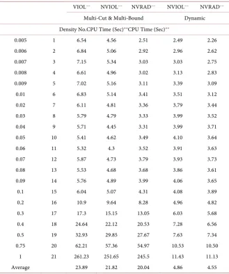
The results of Table 1 for Set 1 compare NVRAD to VIOL, as well as to both a dynamic and non-dynamic version of NVIOL. In addition, the dynamic NVRAD described in Section 2.2 was compared to a non-dynamic NVRAD that applies the multi-cut and multi-bound technique of [18]. The dynamic version was significantly faster. The efficacy of the dynamic approach was further dem-onstrated by the fact that in higher density problems a dynamic version of NVIOL was up to 21 times faster than the multi-cut, multi-bound NVIOL. Overall, dynamic NVRAD was faster than VIOL and NVIOL on every problem instance.

[image:9.595.208.538.115.510.2]

Table 1. CPU times for multi-cut, multi-bound and dynamic active-set approaches on problem Set 1 for random NNLPs with 1000 variables, 200,000 constraints, and

1 5,

ij

a = − bi= −1 10, cj= −1 10.

VIOL−− _NVIOL−− _NVRAD−− _NVIOL−− _NVRAD−− Multi-Cut & Multi-Bound Dynamic Density No.CPU Time (Sec)++_{CPU Time (Sec)}++

0.005 1 6.54 4.56 2.51 2.49 2.26 0.006 2 6.84 5.06 2.92 2.96 2.62 0.007 3 7.15 5.34 3.03 3.03 2.75 0.008 4 6.61 4.96 3.02 3.13 2.83 0.009 5 7.02 5.16 3.11 3.39 3.09 0.01 6 6.83 5.14 3.41 3.51 3.12 0.02 7 6.11 4.81 3.36 3.79 3.44 0.03 8 5.79 4.79 3.33 3.99 3.52 0.04 9 5.71 4.45 3.31 3.99 3.71 0.05 10 5.41 4.62 3.49 4.10 3.64 0.06 11 5.32 4.3 3.52 3.91 3.63 0.07 12 5.87 4.73 3.79 3.93 3.73 0.08 13 5.53 4.68 3.68 3.86 3.61 0.09 14 5.76 4.89 3.99 4.06 3.65 0.1 15 6.04 5.07 4.31 4.08 3.89 0.2 16 10.9 9.64 8.28 4.96 4.82 0.3 17 17.3 15.15 13.05 6.03 5.68 0.4 18 24.64 22.12 20.53 7.28 6.56 0.5 19 32.93 29.85 27.67 7.63 7.34 0.75 20 62.21 57.36 54.97 10.53 10.50

1 21 261.23 251.65 245.5 11.43 11.13 Average 23.89 21.82 20.04 4.86 4.55

++_{Average of 5 instances at each density.} −− _{Used CPLEX presolve = OFF and predual = OFF.}

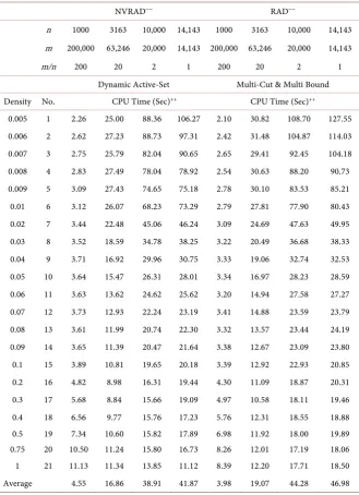
NVRAD over all densities are 19.07 and 16.86 seconds, respectively. For Set 3, dynamic NVRAD is superior to RAD averaging 38.91 seconds compared to 41.87 seconds. Similarly, for Set 4 the averages are 41.87 for NVRAD as com-pared to 46.98 for RAD. Thus the results of Table 2 affirm NVRAD’s ability to add appropriate constraints at each iteration. The results for Set 1 simply reflect how well the prior COST RAD performs when m is very much larger than n.

the optimal combination of RAD and NVRAD in HYBR since an optimal com-bination would likely differ depending on various factors such as density and the ratio m/n.

Table 4, taken from [18], provides a comparison of the posterior COST NVRAD with the standard CPLEX solvers. Comparing the results of Table 4 for the CPLEX solvers with the results for NVRAD in Table 2 shows that NVRAD was significantly faster across virtually all ratios m n and all densities. For example,

[image:10.595.207.537.265.720.2]

the primal simplex was the most robust CPLEX solver, but on the average across all densities the primal simplex took approximately 3 to 14 times more CPU time for the different rations m n than NVRAD. For the dual simplex, the av-

Table 2. CPU times for multi-cut, multi-bound and dynamic active-set approaches on problem Sets 1 - 4 for random NNLPs with aij= −1 5, bi= −1 10, cj= −1 10.

NVRAD−− _RAD−−

n 1000 3163 10,000 14,143 1000 3163 10,000 14,143 m 200,000 63,246 20,000 14,143 200,000 63,246 20,000 14,143

m/n 200 20 2 1 200 20 2 1

Dynamic Active-Set Multi-Cut & Multi Bound Density No. CPU Time (Sec)++ _{CPU Time (Sec)}++

0.005 1 2.26 25.00 88.36 106.27 2.10 30.82 108.70 127.55 0.006 2 2.62 27.23 88.73 97.31 2.42 31.48 104.87 114.03 0.007 3 2.75 25.79 82.04 90.65 2.65 29.41 92.45 104.18 0.008 4 2.83 27.49 78.04 78.92 2.54 30.63 88.20 90.73 0.009 5 3.09 27.43 74.65 75.18 2.78 30.10 83.53 85.21 0.01 6 3.12 26.07 68.23 73.29 2.79 27.81 77.90 80.43 0.02 7 3.44 22.48 45.06 46.24 3.09 24.69 47.63 49.95 0.03 8 3.52 18.59 34.78 38.25 3.22 20.49 36.68 38.33 0.04 9 3.71 16.92 29.96 30.75 3.33 19.06 32.74 32.53 0.05 10 3.64 15.47 26.31 28.01 3.34 16.97 28.23 28.59 0.06 11 3.63 13.62 24.62 25.62 3.20 14.94 27.58 27.27 0.07 12 3.73 12.93 22.24 23.19 3.41 14.88 23.59 23.79 0.08 13 3.61 11.99 20.74 22.30 3.32 13.57 23.44 24.19 0.09 14 3.65 11.39 20.47 21.64 3.38 12.67 23.09 23.80 0.1 15 3.89 10.81 19.65 20.18 3.39 12.92 22.93 20.85 0.2 16 4.82 8.98 16.31 19.44 4.30 11.09 18.87 20.31 0.3 17 5.68 8.84 15.66 19.09 4.97 10.58 18.11 19.46 0.4 18 6.56 9.77 15.76 17.23 5.76 12.31 18.55 18.88 0.5 19 7.34 10.60 15.82 17.89 6.98 11.92 18.00 19.89 0.75 20 10.50 11.24 15.80 16.73 8.26 12.01 17.19 18.06 1 21 11.13 11.34 13.85 11.12 8.39 12.20 17.71 18.50 Average 4.55 16.86 38.91 41.87 3.98 19.07 44.28 46.98

erage CPU across all densities was approximately 15 to 50 times greater than NVRAD over the different ratios. However, the CPLEX barrier method was slightly faster than NVRAD in problem instances with m n=20 and with densities less than 0.02. On the other hand, when the density reached 0.08 for

20

m n= , NVRAD was already more than ten times faster than the barrier

solver. Furthermore, note that average CPU times in Table 4 greater than 3000 seconds (50 minutes) at any density were not reported. This situation occurred for the CPLEX barrier solver for the ratios 1, 2, 20, and 200 with densities at least 0.3, 0.4, 0.5, and 0.75, respectively.

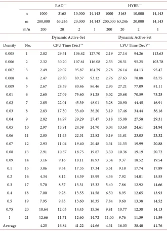
Finally, for large-scale, low-density test problems with n=5000 and

Table 3. CPU times for dynamic HYBR and dynamic RAD on problem Sets 1 - 4 for random NNLPs with a_ij= −1 5, bi= −1 10, cj= −1 10.

RAD−− _HYBR−−

n 1000 3163 10,000 14,143 1000 3163 10,000 14,143 m 200,000 63,246 20,000 14,143 200,000 63,246 20,000 14,143 m/n 200 20 2 1 200 20 2 1

Dynamic Active-Set Dynamic Active-Set Density No. CPU Time (Sec)++ _{CPU Time (Sec)}++

0.005 1 2.02 29.51 106.42 127.70 2.19 27.14 94.26 113.63 0.006 2 2.32 30.20 107.61 116.08 2.53 28.51 95.25 103.78 0.007 3 2.49 29.07 95.87 104.79 2.78 26.14 84.13 95.47 0.008 4 2.47 29.80 89.37 93.12 2.76 27.63 78.88 83.75 0.009 5 2.67 28.59 80.46 86.46 2.93 27.21 77.09 81.11 0.01 6 2.65 27.09 75.60 81.28 3.02 25.68 70.59 75.25 0.02 7 2.85 22.01 45.39 48.01 3.28 20.90 44.45 46.91 0.03 8 2.83 17.30 33.40 36.20 3.19 17.46 34.44 36.18 0.04 9 2.82 14.97 29.29 27.47 3.18 15.08 27.58 29.31 0.05 10 2.97 13.91 24.38 24.70 3.04 13.68 24.61 24.94 0.06 11 2.85 11.43 22.31 22.82 3.19 11.81 23.03 23.32 0.07 12 2.93 11.04 19.40 20.48 3.31 11.55 19.99 20.88 0.08 13 2.91 10.37 18.75 19.87 3.30 10.36 19.19 20.72 0.09 14 3.16 9.16 18.11 18.93 3.34 9.37 18.52 19.54 0.1 15 3.06 9.54 17.35 17.34 3.51 9.18 17.74 17.89 0.2 16 4.34 8.12 14.39 15.99 4.36 7.92 14.01 15.55 0.3 17 5.70 8.57 13.31 15.32 5.40 7.86 12.92 14.66 0.4 18 7.00 9.28 13.55 14.58 6.50 8.95 12.65 13.93 0.5 19 7.95 9.85 13.60 16.35 7.84 9.60 13.38 14.52 0.75 20 10.64 12.05 14.43 15.56 9.81 10.77 12.38 14.13 1 21 12.66 11.71 12.60 14.72 11.00 9.76 11.39 11.59 Average 4.25 16.84 41.22 44.66 4.31 16.03 38.40 41.76

[image:11.595.207.538.264.719.2]

1, 000, 000.

m= Table 5 compares dynamic NVRAD to multi-cut and

[image:12.595.53.538.252.718.2]

mul-ti-bound RAD, VIOL, NVIOL, and NVRAD, as well as to the CPLEX primal simplex, dual simplex, and barrier solvers. Only the prior COST RAD was com-petitive. NVRAD averaged 63.45 seconds overall as compared to 71.79 for RAD. It should be noted that the highest density used in problem Set 5 was 0.0600 since the CPLEX solvers could not solve denser problems of such magnitude in a reasonable amount of time. Average CPU times greater than 2400 seconds (40 minutes) at any density were not reported in Table 5. This situation occurred beginning at some individual threshold density level for each CPLEX solver.

Table 4. CPU times from [18] for CPLEX solvers on problem Sets 1 - 4 for random NNLPs with aij= −1 5, bi= −1 10,

1 10

j

c = − .

Primal+ _Dual+ _Barrier+

n 1000 3163 10,000 14,143 1000 3163 10,000 14,143 1000 3163 10,000 14,143 m 200,000 63,246 20,000 14,143 200,000 63,246 20,000 14,143 200,000 63,246 20,000 14,143

m/n 200 20 2 1 200 20 2 1 200 20 2 1

Density No. CPU Time (Sec)++

0.005 1 7.01 71.02 228.51 309.83 54.84 762.62 1597.24 1169.04 2.36 14.52 240.17 650.83 0.006 2 10.36 77.28 245.60 291.07 60.29 803.97 1607.16 2413.42 2.39 16.30 224.08 666.54 0.007 3 12.98 75.84 219.72 265.09 91.39 876.85 1483.20 1702.47 3.04 18.34 233.55 671.56 0.008 4 15.72 82.01 206.45 239.30 100.06 912.75 1445.54 1236.76 3.90 20.70 232.38 668.82 0.009 5 19.25 80.35 196.72 216.23 114.95 898.99 1375.73 427.95 4.76 22.66 232.23 649.26 0.01 6 21.92 78.50 182.47 216.60 123.49 912.63 1252.05 436.31 5.53 24.29 228.76 650.30 0.02 7 39.90 78.80 118.28 127.59 203.08 963.66 807.29 362.34 17.13 32.08 242.54 711.26 0.03 8 45.42 79.75 98.02 108.60 217.18 1207.76 545.91 723.98 28.79 45.03 266.90 727.61 0.04 9 50.30 78.78 89.75 88.32 248.75 1489.40 450.08 539.92 41.50 62.28 292.15 806.80 0.05 10 55.16 78.92 81.09 82.14 256.49 1746.46 418.69 519.50 53.72 81.32 327.01 837.67 0.06 11 60.34 77.49 77.28 78.27 251.39 2124.31 378.71 409.47 67.58 100.48 359.53 897.58 0.07 12 62.07 78.93 70.44 70.37 251.74 2446.69 310.89 544.15 84.70 125.49 401.72 948.01 0.08 13 62.92 76.96 70.21 69.81 264.48 2799.62 307.25 388.94 99.51 149.37 454.01 1038.86 0.09 14 66.57 79.07 71.46 72.37 258.14 2523.03 718.04 427.95 119.26 186.06 495.28 1153.31 0.1 15 71.00 74.57 67.43 62.64 287.36 2251.10 267.14 436.31 138.67 207.54 539.64 1194.56 0.2 16 87.49 83.12 64.38 62.99 294.39 1450.82 201.73 362.34 379.68 691.77 1298.76 2529.97

0.3 17 94.57 77.91 67.14 66.61 341.44 1280.71 175.16 267.16 657.45 1333.29 2418.75 b

0.4 18 99.33 78.46 73.58 71.48 384.10 1236.30 146.09 233.39 985.86 2076.09 b b

0.5 19 111.30 84.30 86.50 75.62 427.16 1173.49 133.49 208.65 1350.82 b b b 0.75 20 128.26 99.35 115.00 102.51 410.98 1056.18 132.25 181.95 b b b b 1 21 207.55 94.09 393.54 145.96 375.89 411.19 148.90 165.45 b b b b Average 63.30 80.26 134.46 134.45 238.93 1396.60 662.03 626.55 n/a n/a n/a n/a

[image:13.595.55.538.106.498.2]

Table 5. CPU times for NVRAD versus RAD, VIOL, NVIOL, and the CPLEX solvers on problem Set 5 for random NNLPs with 5000 variables, 1,000,000 constraints, and a_ij= −1 5, bi= −1 100, cj= −1 100.

No. Density NVRAD−− _RAD−− _VIOL−− _NVIOL−− _NVRAD−− CPLEX Primal+

CPLEX Dual+

CPLEX Barrier+ Dynamic _{Multi-Cut & Multi-Bound Not Active-Set Methods}

CPU Time (Sec)++ _{CPU Time (Sec)}++ 1 0.0004 6.21 7.54 157.92 73.09 72.19 11.90 14.08 12.31 2 0.0005 9.22 12.26 177.96 100.86 106.31 23.41 29.83 16.61 3 0.0006 11.94 16.51 252.74 75.41 76.12 13.45 107.61 20.45 4 0.0007 15.45 22.19 282.95 92.70 93.64 18.99 176.50 24.60 5 0.0008 20.16 27.66 325.51 108.42 95.22 28.88 257.06 27.43 6 0.0009 23.70 33.24 346.76 120.57 91.06 40.17 339.49 29.80 7 0.0010 28.01 39.81 374.06 141.35 107.34 50.91 427.60 31.73 8 0.0020 70.01 89.57 393.48 222.63 174.78 173.03 1775.03 48.79 9 0.0030 90.09 104.83 368.92 245.17 190.37 244.01 b _61.31 10 0.0040 99.32 113.40 346.56 224.35 183.58 316.53 b _85.60 11 0.0050 103.78 113.17 322.98 215.49 172.42 366.80 b _91.11 12 0.0060 112.15 122.85 320.97 217.81 171.40 443.43 b _112.46 13 0.0070 106.61 116.00 283.16 214.48 160.63 474.40 b _136.03 14 0.0080 100.14 113.05 258.56 184.76 148.74 529.44 b _158.54 15 0.0090 94.43 104.68 229.32 165.47 138.51 566.20 b _198.31 16 0.0100 100.91 112.82 233.08 171.28 137.64 629.59 b _239.87 17 0.0200 76.77 83.83 142.85 106.45 90.60 1134.77 b _899.87 18 0.0300 69.41 76.69 114.25 86.83 76.77 1740.28 b b 19 0.0400 65.87 67.36 103.22 79.26 71.60 1865.70 b b 20 0.0500 63.71 64.58 100.60 80.35 71.87 2159.55 b b

21 0.0600 64.57 65.62 102.05 82.42 74.41 b b b

Average 63.45 71.79 249.42 143.29 119.29 n a n a n a

++_{Average of 5 instances at each density.}b _{Runs with CPU times > 2400 s are not reported.} −−_{Used CPLEX presolve = OFF and predual = OFF.} +_{Used CPLEX}

presolve = ON and predual = ON.

4. Conclusion

the other hand, HYBR appears slightly faster than NVRAD or RAD. The results of this paper provide further evidence that active-set methods may be the fastest approach for solving linear programming problems.

References

[1] Todd, M.J. (2002) The Many Facets of Linear Programming. Mathematical Pro-gramming, 91, 417-436. https://doi.org/10.1007/s101070100261

[2] Dare, P. and Saleh, H. (2000) GPS Network Design: Logistics Solution Using Op-timal and Near-OpOp-timal Methods. Journal of Geodesy, 74, 467-478.

https://doi.org/10.1007/s001900000104

[3] Rosenberger, J.M., Johnson, E.L. and Nemhauser, G.L. (2003) Rerouting Aircraft for Airline Recovery. Transportation Science, 37, 408-421.

https://doi.org/10.1287/trsc.37.4.408.23271

[4] Li, H.-L. and Fu, C.-J. (2005) A Linear Programming Approach for Identifying a Consensus Sequence on DNA Sequences. Bioinformatics, 21, 1838-1845.

https://doi.org/10.1093/bioinformatics/bti286

[5] Stone, J.J. (1958) The Cross-Section Method, an Algorithm for Linear Program-ming. DTIC Document, P-1490.

[6] Thompson, G.L., Tonge, F.M. and Zionts, S. (1996) Techniques for Removing Non-binding Constraints and Extraneous Variables from Linear Programming Problems. Management Science, 12, 588-608. https://doi.org/10.1287/mnsc.12.7.588

[7] Adler, I., Karp, R. and Shamir, R. (1986) A Family of Simplex Variants Solving an

m d× Linear Program in Expected Number of Pivot Steps Depending on d Only.

Mathematics of Operations Research, 11, 570-590.

https://doi.org/10.1287/moor.11.4.570

[8] Zeleny, M. (1986) An External Reconstruction Approach (ERA) to Linear Pro-gramming. Computers & Operations Research, B, 95-100.

https://doi.org/10.1016/0305-0548(86)90067-5

[9] Myers, D.C. and Shih, W. (1988) A Constraint Selection Technique for a Class of Linear Programs. Operations Research Letters, 7, 191-195.

https://doi.org/10.1016/0167-6377(88)90027-2

[10] Curet, N.D. (1993) A Primal-Dual Simplex Method for Linear Programs. Opera-tions Research Letters, 13, 233-237. https://doi.org/10.1016/0167-6377(93)90045-I

[11] Bixby, R.E., Gregory, J.W., Lustig, I.J., Marsten, R.E. and Shanno, D.F. (1992) Very Large-Scale Linear Programming: A Case Study in Combining Interior Point and Simplex Methods. Operations Research, 40, 885-897.

https://doi.org/10.1287/opre.40.5.885

[12] Barnhart, C., Johnson, E., Nemhauser, G., Savelsbergh, M. and Vance, P. (1998) Branch-and-Price: Column Generation for Solving Huge Integer Programs. Opera-tions Research, 46, 316-329. https://doi.org/10.1287/opre.46.3.316

[13] Mitchell, J.E. (2000) Computational Experience with an Interior Point Cutting Plane Algorithm. SIAM Journal on Optimization, 10, 1212-1227.

https://doi.org/10.1137/S1052623497324242

[14] Corley, H.W., Rosenberger, J., Yeh, W.-C. and Sung, T.K. (2006) The Cosine Simp-lex Algorithm. The International Journal of Advanced Manufacturing Technology, 27, 1047-1050. https://doi.org/10.1007/s00170-004-2278-1

[16] Junior, H.V. and Lins, M.P.E. (2005) An Improved Initial Basis for the Simplex Al-gorithm. Computers and Operations Research, 32, 1983-1993.

https://doi.org/10.1016/j.cor.2004.01.002

[17] Corley, H.W. and Rosenberger, J.M. (2011) System, Method and Apparatus for Al-locating Resources by Constraint Selection. US Patent No. 8082549.

[18] Saito, G., Corley, H.W., Rosenberger, J.M., Sung, T.-K. and Noroziroshan, A. (2015) Constraint Optimal Selection Techniques (COSTs) for Nonnegative Linear Pro-gramming Problems. Applied Mathematics and Computation, 251, 586-598.

https://doi.org/10.1016/j.amc.2014.11.080

[19] Saito, G., Corley, H.W. and Rosenberger, J. (2012) Constraint Optimal Selection Techniques (COSTs) for Linear Programming. American Journal of Operations Research, 3, 53-64. https://doi.org/10.4236/ajor.2013.31004

[20] Noroziroshan, N., Corley, H.W. and Rosenberger, J. (2015) A Dynamic Active-Set Method for Linear Programming. American Journal of Operations Research, 5, 526-535. https://doi.org/10.4236/ajor.2015.56041

Submit or recommend next manuscript to SCIRP and we will provide best service for you:

Accepting pre-submission inquiries through Email, Facebook, LinkedIn, Twitter, etc. A wide selection of journals (inclusive of 9 subjects, more than 200 journals)

Providing 24-hour high-quality service User-friendly online submission system Fair and swift peer-review system

Efficient typesetting and proofreading procedure

Display of the result of downloads and visits, as well as the number of cited articles Maximum dissemination of your research work

Submit your manuscript at: http://papersubmission.scirp.org/