The impact of climate mitigation on projections of future drought

Hydrol. Earth Syst. Sci., 17, 2339–2358, 2013 www.hydrol-earth-syst-sci.net/17/2339/2013/ doi:10.5194/hess-17-2339-2013

© Author(s) 2013. CC Attribution 3.0 License.

EGU Journal Logos (RGB)

Advances in

Geosciences

Open Access

Natural Hazards

and Earth System

Sciences

Annales

Geophysicae

Nonlinear Processes

in Geophysics

Atmospheric

Chemistry

and Physics

Atmospheric

Chemistry

and Physics

Atmospheric

Measurement

Techniques

Atmospheric

Measurement

Techniques

Biogeosciences

Open Access Open Access

Biogeosciences

Discussions

Climate

of the Past

Open Access Open Access

Climate

of the Past

Discussions

Earth System

Dynamics

Open Access Open Access

Earth System

Dynamics

Geoscientific

Instrumentation

Methods and

Data Systems

Open Access

_{Geoscientific}

Instrumentation

Methods and

Data Systems

Geoscientific

Model Development

Open Access Open Access

Geoscientific

Model Development

Hydrology and

Earth System

Sciences

Hydrology and

Earth System

Sciences

Ocean Science

Open Access Open Access

Ocean Science

Discussions

Solid Earth

Open Access Open Access

Solid Earth

Discussions

The Cryosphere

Open Access Open Access

The Cryosphere

Natural Hazards

and Earth System

Sciences

Open Access

Discussions

The impact of climate mitigation on projections of future drought

I. H. Taylor1, E. Burke1, L. McColl1,*, P. D. Falloon1, G. R. Harris1, and D. McNeall1 1_{Met Office Hadley Centre, FitzRoy Road, Exeter, EX1 3PB, UK}

*_{now at: Select Statistical Services, Oxygen House, Grenadier Road, Exeter Business Park, Exeter, EX1 3LH, UK}

Correspondence to: I. H. Taylor ([email protected])

Received: 4 October 2012 – Published in Hydrol. Earth Syst. Sci. Discuss.: 7 November 2012 Revised: 15 May 2013 – Accepted: 24 May 2013 – Published: 27 June 2013

Abstract. Drought is a cumulative event, often difficult to define and involving wide-reaching consequences for agri-culture, ecosystems, water availability, and society. Under-standing how the occurrence of drought may change in the future and which sources of uncertainty are dominant can in-form appropriate decisions to guide drought impacts assess-ments. Our study considers both climate model uncertainty associated with future climate projections, and future emis-sions of greenhouse gases (future scenario uncertainty). Four drought indices (the Standardised Precipitation Index (SPI), Soil Moisture Anomaly (SMA), the Palmer Drought Severity Index (PDSI) and the Standardised Runoff Index (SRI)) are calculated for the A1B and RCP2.6 future emissions scenar-ios using monthly model output from a 57-member perturbed parameter ensemble of climate simulations of the HadCM3C Earth System model, for the baseline period 1961–1990, and the period 2070–2099 (“the 2080s”). We consider where there are statistically significant increases or decreases in the proportion of time spent in drought in the 2080s com-pared to the baseline. Despite the large range of uncertainty in drought projections for many regions, projections for some regions have a clear signal, with uncertainty associated with the magnitude of change rather than direction. For instance, a significant increase in time spent in drought is generally pro-jected for the Amazon, Central America and South Africa whilst projections for northern India consistently show sig-nificant decreases in time spent in drought. Whilst the pat-terns of changes in future drought were similar between narios, climate mitigation, represented by the RCP2.6 sce-nario, tended to reduce future changes in drought. In general, climate mitigation reduced the area over which there was a significant increase in drought but had little impact on the area over which there was a significant decrease in time spent in drought.

1 Introduction

Understanding the potential impacts of climate change is es-sential if planned responses to avoid or minimise the neg-ative impacts and take advantage of positive impacts are to be successful. It is important to understand potential sources of uncertainty that may influence the trajectory that the fu-ture climate takes so that informed decisions can be taken. For instance, knowledge of future uncertainties can be fed into a decision-making framework to ensure that responses are appropriate for the range of potential future climates and resultant impacts.

Drought can have far-reaching consequences for agricul-ture, ecosystems, water availability and society (Confalioneri et al., 2007). Drought impacts can include water scarcity, crop failure, wildfires and famines (Sheffield and Wood, 2011). Impacts vary with location and are related to the vul-nerability of a particular system and its capacity to respond to disasters. For example, severe droughts in modern Australia rarely lead to humanitarian disasters because of the capacity of governments and infrastructure to respond appropriately, whereas droughts in parts of Africa are much more likely to lead to humanitarian disasters because of the greater vulner-ability of the affected populations.

meteorological drought is a reduction in precipitation relative to the mean for a particular location; hydrological drought relates to a reduction in the availability of surface and sub-surface water, agricultural drought results from an insuffi-cient supply of water for plant growth and includes soil mois-ture deficit, and lastly, socio-economic drought is essentially a combination of the other types of drought that lead to ad-verse social and economic impacts (Keyantash and Dracup, 2002). Through time, a drought tends to progress from me-teorological to agricultural to hydrological (Sheffield and Wood, 2011). These categories are reflected in the many dif-ferent drought indices that exist, four of which have been used in this study, as outlined in Sect. 3.1, although our study only considers physical droughts (using meteorological, agri-cultural and hydrological drought indices), each of which in-corporate different features of physical droughts (Wilhite and Glantz, 1985).

Climate change may influence the future occurrence of drought. There is high confidence in projections of in-creased precipitation variability that could in turn increase the risk of droughts across many regions (Douville et al., 2002; Wetherald and Manabe, 2002; Burke et al., 2006; Kundzewicz et al., 2007). Observations have shown an in-crease in the severity and duration of droughts over larger areas since the 1970s (IPCC, 2007). More intense and longer droughts have also been observed in some semi-arid and sub-humid regions, including Southern Europe and West Africa (IPCC, 2012), while droughts have become less frequent, less intense, or shorter in some regions such as central North America and northwestern Australia. However, these find-ings were largely based on studies using the Palmer Drought Severity Index (PDSI) and the reported increases in global drought may have been overestimated because of the simpli-fied calculation of potential evaporation used in the PDSI. Calculations based on the underlying physical principles, considering changes in available energy, humidity and wind speed, suggest little change in drought over the past 60 yr (Sheffield et al., 2012).

The regions which have already experienced increasing drought hazards may therefore be particularly sensitive to any projected increases in physical drought hazards. It is con-sidered likely that the extent of drought-affected areas will increase in the future with climate change (Kundzewicz et al., 2007). Temperature, precipitation and evapotranspiration are major drivers of drought. Temperature and evapotranspi-ration are projected to increase over most land areas, while increases in global mean precipitation are projected, but with strong regional differences, including a projected decrease in precipitation in sub-tropical regions and increases at high latitudes and in the tropics (Kundzewicz et al., 2007). How-ever, there is greater uncertainty associated with projections of precipitation than those for temperature (Meehl et al., 2007). Evaporative demand is also likely to increase every-where. The regions where there is most confidence in fu-ture physical drought increases include southern Europe and

the Mediterranean, central Europe, central North America, Central America and Mexico, northeast Brazil, and southern Africa (IPCC, 2012).

However, drought is not solely affected by climatic drivers, and non-climatic drivers such as population changes, land use and water management have a large influence on water availability and hence drought (Kundzewicz et al., 2007). As these will almost certainly change in the future, they need to be taken into account to gain a complete understanding of fu-ture drought events and their impacts, although these factors are not included in the present study, which focuses only on physical drought hazards (using agricultural, meteorological and hydrological indices).

Improving an understanding of uncertainties in the water– climate interface was identified as a research priority in cent Intergovernmental Panel on Climate Change (IPCC) re-ports (Kundzewicz et al., 2007; Bates et al., 2008). Model projections of future climate change contain uncertainty due to three key sources: internal (or natural) variability, mod-elling uncertainty, and emissions uncertainty (Hawkins and Sutton, 2009). The dominant source of uncertainty varies with variable, region and time horizon (Hawkins and Sut-ton, 2009). In the case of global temperature changes, in-ternal variability is the dominant source of uncertainty on short-term (decadal) timescales; emissions become increas-ingly important for lead times beyond around 40 yr, and mod-elling uncertainty has a larger influence on longer-term pro-jections (end of the century). The total uncertainty increases with time (Hawkins and Sutton, 2009). However, the dom-inant source of uncertainty also depends strongly on region and on the variable considered (Hawkins and Sutton, 2011). The aim of the present study is to assess the impact of cli-mate mitigation policies on future drought projections. In this study we include modelling and emissions uncertainty through the use of a perturbed parameter ensemble of the HadCM3C Earth System model (Lambert et al., 2012) and two future emissions scenarios as detailed in Sect. 2. Inter-nal variability is not assessed in this study. This study differs from the earlier, related studies of Burke et al. (2006) and Burke and Brown (2008) in that it uses a different ensem-ble of climate models driven by two future climate scenarios, and applies a range of plus the SRI index was added in the present study.

Additional uncertainties arise during impacts assessments related to the impact itself. In the case of drought, uncer-tainties are often associated with the choices around how a drought is defined. This includes the type of drought (for ex-ample meteorological, hydrological or agricultural), and the severity, duration, location and frequency of the drought.

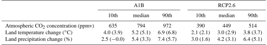
Table 1. The end-of-century range of atmospheric CO₂concentration (extract from Booth et al., 2012, 2013), temperature and precipitation given by the ESE simulations for the SRES A1B and RCP2.6. CO2is the 2099 value. Temperature and precipitation are based on the end-of-century 10 yr average (2070–2099) relative to the 1961–1990 average, over all global land points. Values in parentheses exclude cold regions as described in the text.

A1B RCP2.6

10th median 90th 10th median 90th

Atmospheric CO2concentration (ppmv) 635 794 972 390 449 514

Land temperature change (◦C) 4.0 (3.9) 5.2 (5.1) 6.9 (6.8) 2.1 (2.1) 3.0 (2.9) 3.8 (3.7) Land precipitation change (%) 2.5 (−0.0) 5.4 (3.3) 7.4 (5.7) 3.0 (1.6) 4.2 (3.1) 6.4 (5.1)

drought and can be used as an indicator of agricultural drought; the widely used Palmer Drought Severity Index (PDSI), is also considered to be mostly an indicator of mete-orological drought; and the Standardised Runoff Index (SRI) represents hydrological drought. The choice of threshold be-low which a drought is measured reflects drought severity and may influence the interpretation of future drought pro-jections. To address this we have calculated the time spent in drought below five different thresholds.

The results are analysed to examine whether there is a change in the proportion of time spent in drought in the 2080s relative to the baseline period. Where there are significant differences, we assess the percent of the land surface with either an increase or decrease in the time spent in drought for the different thresholds, indices, future scenarios and cli-mate model ensemble members. The use of an ensemble of climate model projections, and two future scenarios enables the assessment of uncertainties in future drought projections from these two sources. It should be noted that a small uncer-tainty range does not necessarily imply greater confidence in the projections, for example if the model/index provides in-accurate projections.

2 Climate model simulations

In this study we use a large ensemble of climate change simu-lations with different configurations of HadCM3C (Booth et al., 2012, 2013), a coupled atmosphere-ocean-carbon cycle Earth system model. The model is configured from HadCM3 (Gordon et al., 2000), a widely studied coupled ocean-atmosphere model used by the Met Office Hadley Centre to provide input for the IPCC Third and Fourth Assessment Re-ports. In the HadCM3C configuration, the model incorpo-rates a fully interactive (land and ocean) carbon cycle with dynamic vegetation and an interactive sulphur cycle scheme, in addition to the standard physical representations of the at-mosphere, ocean and land surface. Flux adjustments are used to restrict historical simulation biases in sea surface temper-ature and salinity, following Collins et al. (2011).

In HadCM3C, runoff and soil moisture are calculated by the Met Office Surface Exchange Scheme Version 2 (MOSES2 – Essery et al., 2001, 2003; Cox et al., 1999).

There are there are four soil layers in MOSES2, each with a temperature, and moisture content with thicknesses from the surface downwards, of 0.1, 0.25, 0.65 and 2.0 m. The soil hy-drology component of MOSES is based on a finite difference form of the Richards equation (Richards, 1931). The water flux which enters the soil at the surface is the sum of the throughfall and snowmelt minus surface runoff. The lower boundary condition assumes free drainage (Cox et al., 1999). Transpiration through plants extracts soil moisture directly from each soil layer via roots and bare soil evaporation de-pletes moisture from the top soil layer. The ability of roots to access moisture in each soil layer is determined by a root density distribution; root density is assumed to follow an ex-ponential distribution with depth.

The design and setup of the Earth System Ensemble (ESE) is fully described by Lambert et al. (2012). The ESE is a de-velopment of a series of previously investigated perturbed parameter ensemble (PPE) experiments (e.g. Murphy et al., 2009; Collins et al., 2011; Booth et al., 2012, 2013), which investigated the uncertainties associated with different as-pects of the climate system. The ESE brings together these ensembles to simultaneously explore parametric uncertainty in the atmosphere, ocean, land carbon cycle and sulphur cy-cle processes in this Earth system model. An ensemble of 57 members has been created and driven using two future emissions scenarios; the IPCC Special Report on Emissions Scenarios (SRES) A1B scenario (Nakicenovic et al. 2000), a “business as usual” emissions scenario, and Representative Concentration Pathway 2.6 (RCP2.6; Moss et al., 2010), an aggressive mitigation scenario. Note that these two scenarios are from different “families”, but were the datasets available from the ESE. The simulations also include appropriate his-torical periods. Comparison of these scenarios allows us to understand what changes and climate impacts might be mit-igated by a change in behaviour, and also how much climate change we are already committed to because of the delayed response of the Earth System.

concentration. In Lambert et al. (2012) it is shown that inter-actions between uncertainties play a significant role in deter-mining the spread of responses in global mean surface tem-perature. The ESE also explores a wide range of regional re-sponse, and therefore provides a useful resource for the pro-vision of regional climate projections and associated uncer-tainties. It is important, however, to note that the ensemble was designed to sample a large range of uncertainty, rather than to produce a set of equally plausible projections. It is more appropriate therefore to interpret the ESE projections as a spread of possible outcomes, rather than a set of likely futures.

3 Methods

Results were analysed for 2070–2099 (“the 2080s”) and compared with the baseline period (1961–1990).

3.1 Application of drought indices

Four indices of drought are calculated and analysed, the SPI, the SRI, the SMA and the PDSI, using an approach similar to that of Burke and Brown (2008). Details of each of these in-dices and their application in the present study are provided below. As noted in the introduction, the indices chosen rep-resent different kinds of drought, and exhibit different un-certainties because they are related with processes that are either difficult to observe over large areas (e.g. soil mois-ture, runoff) or difficult to parameterize due to lack of pro-cess knowledge.

3.1.1 Standardised Precipitation Index (SPI) and Standardized Runoff Index (SRI)

The SPI was developed by McKee et al. (1993) and has re-cently been adopted as the standard meteorological drought index by the World Meteorological Organisation (WMO) (Sheffield and Wood, 2011; Hayes et al., 2011). It is based on the probability of precipitation for a particular location (Keyantash and Dracup, 2002) where observed or modelled precipitation is calculated as a deviation from the longer-term normal (Sheffield and Wood, 2011). The index can be ap-plied to multiple timescales of accumulation, typically rang-ing from one to 48 months. This represents the variation of the impacts of reduced precipitation with event duration (Sivakumar et al., 2010).

The present study predominantly uses a twelve-month ac-cumulation period, although Vidal et al. (2012) note that the response of drought to climate change can be highly sensitive to the timescale considered. We therefore also include SPI calculated on a range of different timescales (1, 3, 12, 18 and 24 months). Because the SPI is based solely on precipita-tion, which is readily available from both observed and mod-elled data, and is relatively simple to calculate, it is widely applicable for drought assessment (Sivakumar et al., 2010).

This is particularly true for developing countries where data may be limited. This drought index is only really applicable to meteorological drought as it only includes precipitation and does not account for interactions with the land surface or temperature.

For this study, the SPI is calculated following the approach of Burke and Brown (2008), from climate model monthly precipitation that was normalised around the baseline thirty-year distributions for each model grid square. Following Burke and Brown (2008), the SPI is estimated by transform-ing the long-term precipitation distribution for each loca-tion to a normal distribuloca-tion (Guttman, 1999). The localoca-tion- location-specific parameters used to transform the baseline precipita-tion distribuprecipita-tion were also used to transform the future pre-cipitation distribution.

The SRI was calculated in an analogous fashion to the SPI but using the modelled monthly mean runoff time series for each grid cell. This is a recently adopted index (Shukla and Wood, 2008) which can be used to evaluate hydrological droughts or as a proxy for river discharge (e.g. Joetzjer et al., 2012).

3.1.2 Soil Moisture Anomaly (SMA)

The SMA is a useful index of agricultural drought, as it re-flects the moisture available for plant usage. The available soil moisture, calculated within a global circulation model (GCM), is a crucial component of the hydrological cycle that essentially involves a balance between precipitation, runoff, and evaporation (including evapotranspiration by vegetation; Sheffield et al., 2009). Although the SMA is not widely used as an operational drought index because observations of soil moisture are not collected over large areas, it can provide a good indication of modelled agricultural drought. It also has the advantage of being calculated within the coupled climate model so will inherently include CO2physiological effects if these are included in the climate model and the effect of any included feedbacks on climate projections (as in the present study).

For this study the SMA is calculated from the direct model output of soil moisture using the approach of Burke and Brown (2008). Soil moisture anomalies are calculated for the top 1m of soil, using data for the first three soil layers in the HadCM3C model, having thicknesses from the top of 0.1, 0.25, and 0.65 m. The SMA was calculated at timescales of 12 months, for the top 1m of the soil by subtracting the soil moisture climatology (Burke and Brown, 2008), and the re-sulting data were not normalised by the standard deviation.

3.1.3 Palmer Drought Severity Index (PDSI)

Change in mean

Proportion of time spent in drought

Probability

Baseline 10th percentile

Baseline 20th percentile

Change in shape

Proportion of time spent in drought

Probability

Baseline 10th percentile

Baseline 20th percentile

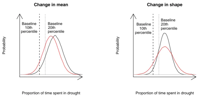
Fig. 1. Schematic of drought threshold. The black line represents a sample baseline distribution and the red line a sample future distribution.

Wood, 2011). It was first developed by Palmer (1965), based on limited data from the United States to give a measure of the “cumulative departure of moisture supply” (Keyantash and Dracup, 2002). Based on the water balance equation for a particular location (Sivakumar et al., 2010) the PDSI is es-sentially a balance between incoming and outgoing water us-ing a two-layer, bucket-type scheme with climatological cal-ibrations for a specific location in space and time (Burke et al., 2006). Like the SPI, the PDSI values are dimensionless and generally range between+4 and−4 with any value be-low zero being indicative of water shortage (Keyantash and Dracup, 2002).

The PDSI is particularly sensitive to changes in tempera-ture because of the rather simplistic representation of poten-tial evaporation that is commonly used (Sheffield and Wood, 2011). This means that observed and projected global tem-perature increases due to climate change may result in a much stronger increase in drought than is considered phys-ically plausible. The Penman–Monteith potential evapora-tion model is an alternative approach to calculating poten-tial evaporation that is considered more physically plausible than the Thornthwaite model (van der Schrier et al., 2011). However it does not necessarily reduce the strong tempera-ture sensitivity of the PDSI sufficiently (van der Schrier et al., 2011).

Several other aspects of the PDSI have been criticised, in-cluding the lack of spatial consistency (Sheffield and Wood, 2011); the limited representation of vegetation and roots; an inability to account for frozen processes (Burke et al., 2006); the underestimation of runoff; and the lack of soil moisture heterogeneity across regions (Sivakumar et al., 2010).

In this study the self-calibrated PDSI is used. This was developed in 2004 (Wells et al., 2004) to improve the abil-ity to make spatial comparisons as the calibrations are based on local conditions rather than the fixed values of the orig-inal PDSI (Dai, 2011). The calculation of the PDSI is rela-tively complex and requires monthly data for precipitation,

temperature, the available water holding capacity of the soil, and potential evaporation. Potential evaporation is calculated with the Penman–Monteith equation (from temperature, rel-ative humidity, pressure, wind and short- and longwave ra-diation), following the methodology of Burke et al. (2006). The calculation of potential evaporation is strongly sensitive to formulation choices (e.g. timestep) and to the quality of in-put variables (Kay and Davies, 2008). The PDSI has a mem-ory of the order of 12 months, resulting in the use of this timescale for the other indices (Burke and Brown, 2008). Calibration parameters determined for each location under baseline climate conditions were held constant when calcu-lating the PDSI for future conditions.

3.1.4 Drought thresholds

then converted into a proportion of time over the thirty years spent in drought for each drought threshold.

3.2 Analysis

Analysis and communication of results from a large ensem-ble, as used here, presents certain challenges. Rather than presenting ensemble mean projections, here we provide an alternative presentation based around a typical “exemplar” member of the ensemble. The concept of model consensus (Kaye et al., 2012; McSweeney and Jones, 2013) is also used to analyse the degree of agreement across the different model projections. Unlike the ensemble mean, a representative ex-emplar model projection provides joint patterns of climate response for several climate variables that corresponds to a physically consistent solution to the modelled representation of climate system processes. Variability is also retained in the exemplar, which is important for realistic climate impact studies. This approach enables the same model to be traced across the three drought indices, different drought thresholds and significant increases and decreases whilst maintaining the model’s spatial characteristics.

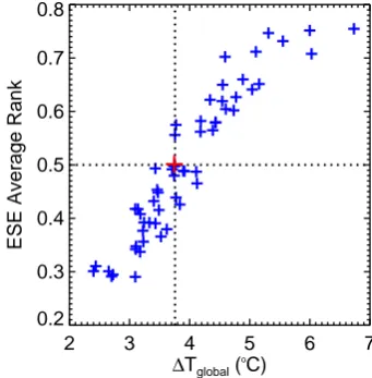
The exemplar member was chosen on the basis that, on average, across selected regions and variables, it possesses the median response of the ensemble. Specifically, for a selection of 24 countries, including the nineteen G20 na-tions (Vestergaard, 2011) and five others, the ESE members are ranked for each of the four seasons by their projected temperature and percentage precipitation change at the end of the 21st century in response to the A1B emissions sce-nario. These ranks, normalised by the number of runs so that 0.0 corresponds to coldest/driest, 1.0 to hottest/wettest, and 0.5 to the median, were then averaged to give an average rank for each member, assuming equal weight for each country. In Fig. 2 a scatter plot of the average rank and the global temperature response is shown for the ESE members. Not surprisingly, a strong relationship between these two quan-tities is obtained. Several members lie close to the median. The exemplar member is chosen in preference to other simi-larly ranked candidates on the basis that it possesses a small variance in rank. It is worth noting that although on aver-age the selected member is close to the median, this does not preclude that for some regions and variables, the ex-emplar can be far from the median. Country responses are used here to select the exemplar since detailed climate pro-jections for these countries, based on the ESE models that comprehensively sample earth system modelling uncertainty, will shortly be produced. Therefore this exemplar approach will maintain consistency with these and enable comparison with other related studies using the ESE (e.g. Lambert et al., 2012; Hartley et al., 2013; Murphy et al., 2013). However, we note the following limitations: (a) our study has a global fo-cus, and the exemplar selected on countries may bias toward larger countries and regional biases; and (b) selection of the average response over countries may limit applicability at the

2 3 4 5 6 7

∆Tglobal (

o

C) 0.2

0.3 0.4 0.5 0.6 0.7 0.8

ESE Average Rank

Fig. 2. The ESE members ranked by their A1B end-of-century tem-perature response and percentage precipitation change, averaged over the four seasons for 24 selected countries as a function of their 2080–2099 annual global temperature response with respect to 1961–1990. The exemplar member selected to show a represen-tative median response is marked in red.

regional scale where drought assessments are useful (and po-tentially used). Discussion of the regional behaviour of the ESE is included in Murphy et al. (2013).

For each ensemble member, future scenario, drought met-ric and threshold we analyse future projections of the pro-portion of time spent in drought in the period 2070–2099 (representative of the 2080s) compared to the baseline period 1961–1990. The annual proportion of time spent in drought for the baseline and the 2080s is calculated in each case and for each model grid cell. While time in drought is the most basic drought characteristic, the final impact often depends on spatio-temporal characteristics (Vidal et al., 2010).

To test whether there is a significant difference between the two time periods, a Wilcoxon–Mann–Whitney test is ap-plied (Wilks, 2006). This is a non-parametric statistical test with the null hypothesis that two data samples are drawn from the same distribution. The underlying principle of the Wilcoxon–Mann–Whitney test is exchangeability; if the two samples of data from the baseline and the 2080s are not dif-ferent, then each data point is as likely to be from the baseline period as the 2080s. The test statistic pools the data, ranks it and sums the ranks from each time period separately. If the sums of the ranks in the two time periods are sufficiently dif-ferent in magnitude, the null hypothesis is rejected and the two are deemed to be significantly different. In this case a two-sided alternative hypothesis is applied (i.e. the difference between the two time periods could be positive or negative) and the test applied at the 5 % probability level.

the approach of Deichmann and Eklundh (1991), global cold regions are defined as grid cells where the temperature is less than 0◦_{C for more than six months of the year and where less} than three months of the year have temperatures greater than 6◦C. We use the mean of the thirty-year average tempera-ture for the 1961–1990 baseline, averaged across ensemble members of the A1B scenario, as the basis for these calcu-lations. Although in practice, each model ensemble mem-ber would have a unique cold region using the above defi-nition, for internal consistency we use a standard region for all calculations.

To summarise this information over the whole ensemble we use a consensus mapping approach (Kaye et al., 2012). We calculate and map the proportion of ensemble members that exhibit a significant increase, decrease, or no significant change in proportion of time spent in drought (McSweeney and Jones, 2013; Knutti et al., 2010). This provides a mea-sure of agreement on the signal of change (or no change) for different regions around the world and across the ensemble. The consensus maps (Fig. 5) are only presented for 10th per-centile calculations.

4 Results

Here we present our results for the proportion of time spent in drought for the four drought indices, two emissions scenar-ios, five drought thresholds and fifty seven ensemble mem-bers analysed. We first outline how key climate variables are projected to change by the end of the 21st century, both spatially and temporally, to illustrate some of the driving processes behind changes in drought occurrence. We then present the significant changes in time spent in drought in the 2080s compared to the baseline period for both future scenarios.

4.1 Climatic variables

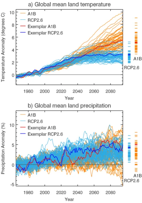
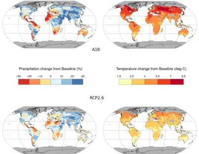
Both temperature and precipitation influence the processes leading to drought events so understanding how those vari-ables are projected to change can help understand the pro-cesses involved in the projected changes in drought indices. In Fig. 3 we therefore present changes in annual mean land surface air temperature, and percentage change in annual mean land precipitation for the two future scenarios. Figure 4 shows the spatial variation in the change in these two quan-tities for the exemplar simulation. Both figures are presented for the same area of the land surface as the drought indices, i.e. cold regions are excluded as defined in Sect. 3.2.

Both future scenarios show a similar projected increase in global average land temperature until the 2040s. After this time, temperatures for the RCP2.6 scenario stabilise, while for the A1B scenario a continued increase is pro-jected. The range of projected temperature changes across the model ensemble is much larger for the A1B scenario

Fig. 3. Annual mean temperature (a) and percentage precipita-tion (b) anomalies (with 5 yr smoothing) from 1961 to 2099 (rel-ative to the 1961 to 1990 average) averaged over land points, ex-cluding cold regions, for the ESE simulations. The A1B future sce-nario is shown in orange and RCP2.6 is shown in blue (individial lines represent individual models). The two exemplar simulations are shown in red (A1B) and dark blue (RCP2.6) respectively. The range of the ensemble is shown to the right of each plot, with the final 30 yr average (2070–2099) for each ensemble member shown for each future scenario.

than for the RCP2.6 scenario; a wider range of responses is expected given the larger forcing in the A1B simulations. Projections for the percentage change in global average land precipitation also show an increase by the end of the century for both emissions scenarios, although the projected change does span zero. The RCP2.6 scenario gives a narrower range of precipitation increases by the end of the century than the A1B scenario ensemble and lies completely within the range of the A1B scenario.

Fig. 4. Precipitation (left panels) and temperature (right panels) anomalies for the 2080s (1970–2099) from the baseline 1961–1990 for the exemplar model of the ESE for A1B (top panels) and RCP2.6 (bottom panels) future scenarios. Grey regions represent the excluded cold regions.

regional patterns. Drying is projected in Southern Europe, the Mediterranean, northern Africa, southern Africa, Central America, across the Amazon, Chile, and southern and eastern Australia, whilst wetting is projected for all other regions.

4.2 Significant changes in time spent in drought

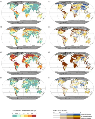
Future projections of drought in the 2080s for the exemplar model and the ensemble consensus are shown in Fig. 5 for the A1B scenario and Fig. 6 for the RCP2.6 scenario for each of the four drought indices, for the 10th percentile calculations only. Using the significance testing described in Sect. 3.2, maps of the proportion of ensemble members that exhibit a significant increase, decrease or no significant change in the proportion of time spent in drought are shown in the right column of both figures. The proportion of models agreeing on a significant decrease, no significant change or a signifi-cant increase in drought is indicated by shading (the darker the shade the greater the agreement). White represents areas where less than 50 % of models agree (Kaye et al., 2012).

For the A1B emissions scenario there are clear differ-ences in drought projections between drought indices, both spatially and in terms of magnitude and direction of the

projected change. More models agree on significant in-creases for PDSI drought, whilst projections of SRI drought show the least model agreement across the ESE model en-semble for either significant increases or decreases. For some regions there is a consistent signal across the SPI, PDSI and SMA drought indices for both significant increases and de-creases in time spent in drought. For instance, significant in-creases in time spent in drought in the 2080s are projected for Central America, the Amazon, southern Chile, the Mediter-ranean, northwestern Africa and parts of South Africa for these three drought indices. There is also some indication of a significant increase in the SRI drought for these regions. In general, projections of PDSI drought have the strongest model agreement and largest spatial extent across those re-gions. Significant decreases were projected for northern In-dia, parts of central Asia and parts of East Africa for all four drought indices, with the SPI showing the largest area with significant decreases in time spent in drought.

Fig. 5. The proportion of time spent in drought for three drought indices from the ESE for the A1B future scenario in the 2080s (2070–2099), exemplar model (left) and model agreement of significant changes (right). (a) and (b) are the SPI, (c) and (d) are for the SMA; (e) and (f) are for the PDSI; and (g) and (h) are for the SRI. Grey areas represent the excluded cold regions. Results shown are for the 10th percentile calculations only.

in those regions. This broadly coincides with regions that are projected to experience future increases in precipitation (Fig. 4) which is directly reflected in the SPI, as it is based solely on precipitation. The difference between the SPI and PDSI/SMA projections in high latitudes is likely to be due to high-latitude temperature amplification, since SPI does not

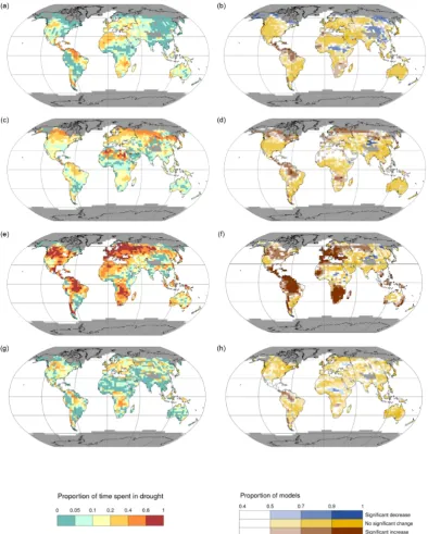
Fig. 6. The proportion of time spent in drought for three drought indices from the ESE for the RCP2.6 future scenario in the 2080s (2070– 2099), exemplar model (left panels) and model agreement of significant changes (right panels). (a) and (b) are the SPI, (c) and (d) are for the SMA; (e) and (f) are for the PDSI; and (g) and (h) are for the SRI. Grey areas represent the excluded cold regions. Results shown are for the 10th percentile calculations only.

projections using the SMA and PDSI than precipitation changes. The SRI shows little agreement between models at these latitudes.

Projections for some regions show no significant change in the time spent in drought in the future. This is because the increases or decreases in time spent in drought given by the drought indices are not different enough from the

based on both surface and subsurface runoff from the whole soil profile. Subsurface runoff changes are likely to be more damped (and less strongly related to changes in upper layer soil moisture) than surface runoff changes. This may partly explain the weaker signals seen in the SRI compared to the SMA. In some cases, regions with no significant change cor-respond to regions with lower model agreement for precip-itation changes, as was the case for the other indices. How-ever, the precipitation projections shown are for all changes rather than just those that are significantly different from the baseline.

Figure 5 (left panels) shows the proportion of time spent in drought in the 2080s for each model grid square for the A1B exemplar model (excluding the cold regions). For the 10th percentile drought (as shown here) values greater than 0.1 indicate an increase in time spent in drought com-pared to the baseline and values below 0.1 indicate a de-crease. For the exemplar model, the PDSI suggests high pro-portions of time spent in drought (>80 %) for some regions, which is greater than the values found by Burke et al. (2006) and Burke and Brown (2008). This may be due to the greater warming in the ESE compared to the climate models studied by Burke et al. (2006) and Burke and Brown (2008). Similar regional patterns of change to the significance plots are evi-dent, particularly for the strongest increases in time spent in drought. These plots illustrate the change in the proportion of time spent in drought across the entire globe rather than just where the change is significant (as the model agreement plots do) so they include the projected changes for this ensemble member for regions that show no significant change across the model ensemble. For the exemplar model ensemble mem-ber, the regions corresponding to no significant change in the model agreement plots (Fig. 5, right panels) mainly show de-creases in time spent in drought in the future.

Projections for the RCP2.6 scenario are regionally simi-lar to those for the A1B scenario, although with less model agreement, smaller magnitude of change, and a smaller area showing significant change (see Fig. 6).

4.3 Uncertainties in future drought projections

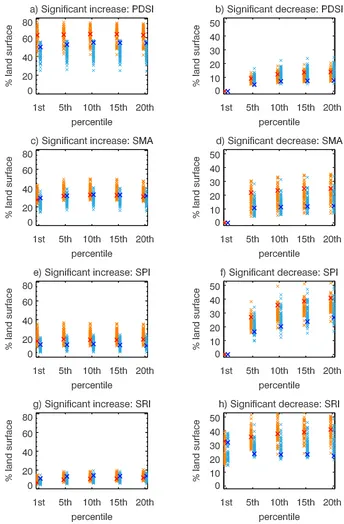
Uncertainties in future drought projections were represented by calculating the percentages of the land surface (excluding cold regions) with a significant increase and decrease in the time spent in drought in the 2080s (as defined in Sect. 3.1). These are shown in Fig. 7.

Of the four drought indices, PDSI drought shows the largest proportion of the land surface with a significant in-crease in drought (approximately 60 % for the A1B sce-nario and between 50–60 % for the RCP2.6 scesce-nario) and the smallest proportion with a significant decrease (Fig. 7). SRI drought shows the lowest percentage of the land surface with a significant increase in time spent in drought (with values ranging between 15–50 % for the A1B scenario and similar for the RCP2.6 scenario) and the highest with a significant

decrease. As Fig. 5 shows, both SPI and SRI projections tend to show more significant decreases in time spent in drought whilst the SMA and PDSI projections tend to show more sig-nificant increases. This would explain, for example, the lower percentage of the land surface with a significant increase for SRI and the higher significant decreases found with the SRI (as in Fig. 7). Projections for SMA drought fall between the small increase in SRI and SPI drought and the large increase in the PDSI drought, with between 20 and 50 % of the land surface projected to experience a significant increase in the time spent in drought under the A1B scenario and between 15 and 40 % under the RCP2.6 scenario. Projections of both SMA and PDSI drought indicate that more of the land surface could have a significant increase in time spent in drought in the 2080s than a significant decrease.

The spread across the ensemble (modelling uncertainty) varies with drought index, future scenario and to a lesser extent, drought threshold. The smallest ensemble spread is found for significant increase in SRI drought, most likely because it is only a small change and the largest ensemble spread occurs with significant increases in PDSI drought. Figures 5 and 6 show that for the PDSI, significant increases cover larger areas of the globe than the other two drought indices and significant decreases cover less. The ensemble members show different behaviour across the drought indices and for significant increases and decreases in time spent in drought.

In all cases the projections for the two future scenar-ios overlap to varying degrees. The least overlap occurs in the projections of significant increases in PDSI drought. As Fig. 5 shows, under the A1B scenario large areas of the globe have significant increases for PDSI, whilst under the RCP2.6 scenario, there are more areas with no significant change. As PDSI is influenced by temperature, this appears to be related to the higher temperature changes projected under the A1B scenario (Fig. 4). For both future scenarios the projections of significant decreases in SPI, SRI and PDSI drought almost completely overlap. Broadly speaking, the spatial patterns of the two emissions scenarios are similar, as shown in Figs. 5 and 6, with the RCP2.6 scenario having fewer grid squares with significant changes and less model agreement where they do occur. The magnitude of change is therefore lower for RCP2.6 even if that change occurs over roughly the same number of grid squares as it does for the A1B scenario.

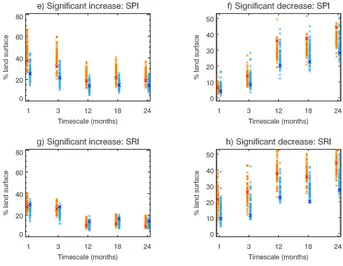
Fig. 8. The percent of the land surface (non-cold areas) with significant changes (as defined in Sect. 3.1) in the time spent in drought in the 2080s (2070–2099) as given by the ESE (increases – left column, and decreases – right column) for the SPI: (a), (b); and SRI: (c) and (d) at the different integration timescales. The A1B future scenario is shown in orange and RCP2.6 shown in blue. The crosses represent individual model responses with the exemplar ensemble member marked larger symbols in red (A1B) and dark blue (RCP2.6).

Figure 8 shows the dependence of the SPI and SRI drought on the timescales. Any changes at the 12-, 18- and 24-month timescales are very similar for both drought indices, suggest-ing that the SPI and SRI shown in Fig. 7 are more represen-tative of annual timescales and above. At the 1-and 3-month timescales, the ensembles generally show more areas with a significant increase in drought and a smaller area with a significant decrease in drought. Model spread within the en-sembles is also larger at these timescales.

5 Discussion

5.1 Drought indices

We find considerable differences in future projections of time spent in drought between the four drought indices used in this study, the SPI, SRI, SMA and PDSI. The many drought indices that have been developed tend to represent different components of the hydrological cycle and types of drought that can occur (Sivakumar et al., 2010; Keyantash and Dracup, 2002; Sheffield and Wood, 2011). Different drought indices have been shown to give a range of outcomes of drought occurrence. For example, Burke and Brown (2008) compared several drought indices projections of the change in percent area of the land surface under a doubling of CO2 in moderate drought and found that the SPI gave changes

ranging from−5 to 10 %, the PDSI gave changes from 10 to 35 %, and the SMA gave changes from 5 to 20 % approxi-mately; similar findings were made by Joetzjer et al. (2012) who compared three drought metrics over two river basins. This may be related to the aspect of the hydrological cycle that they represent, or the strengths and weaknesses of the formulation of the index itself (as detailed in Table 2). Resul-tant differences in the drought metrics, time series of runoff, precipitation, soil moisture, and the PDSI, are, as expected, primarily driven by differences in the climatic variables upon which they are based, particularly precipitation and tempera-ture (Burke, 2011). Burke (2011) showed that metrics based on precipitation, soil moisture and the PDSI were similarly sensitive to precipitation, whilst the response to changes in temperature was metric dependant. The PDSI was the most influenced by changes in temperature, soil moisture to a lesser extent, and precipitation was shown to be independent of temperature changes. Whilst the current study uses the SPI rather than a time series of precipitation directly from the model, our results largely agree with these findings. This is expected since the SPI and precipitation percentile thresholds are equivalent.

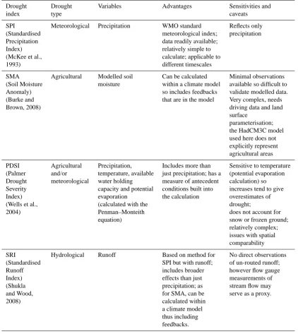
Table 2. Summary of the three drought indices applied in this study.

Drought Drought Variables Advantages Sensitivities and

index type caveats

SPI Meteorological Precipitation WMO standard Reflects only

(Standardised meteorological index; precipitation

Precipitation data readily available;

Index) relatively simple to

(McKee et al., calculate; applicable to

1993) different timescales

SMA Agricultural Modelled soil Can be calculated Minimal observations (Soil Moisture moisture within a climate model available so difficult to

Anomaly) so includes feedbacks validate modelled data.

(Burke and that are in the model Very complex, needs

Brown, 2008) driving data and land

surface

parameterisation; the HadCM3C model used here does not explicitly represent agricultural areas

PDSI Agricultural Precipitation, Includes more than Sensitive to temperature (Palmer and/or temperature, available just precipitation; has a (potential evaporation Drought meteorological water holding measure of antecedent calculation) so Severity capacity and potential conditions built into increases tend to give

Index) evaporation the calculation overestimates of

(Wells et al., (calculated with the drought;

2004) Penman–Monteith does not account for

equation) snow or frozen ground;

relatively complex; issues with spatial comparability

SRI Hydrological Runoff Based on method for No direct observations

(Standardised SPI but with runoff; of un-routed runoff;

Runoff includes broader however flow gauge

Index) effects than just measurements of

(Shukla precipitation; as stream flow may

and Wood, for SMA, can be serve as a proxy.

2008) calculated within

a climate model thus including feedbacks.

the drought indices. This is particularly the case for the SPI, which depends solely on regional precipitation, for which projected changes are generally more uncertain than those for temperature, as are those for soil moisture (Falloon et al., 2011). Contrastingly, projections of PDSI drought, which are largely influenced by temperature changes, show large areas of the globe with a significant increase in drought. The PDSI is known to be particularly sensitive to temperature, largely due to its representation of (and the influence of tempera-ture on) evapotranspiration (Sheffield and Wood, 2011; van der Schrier et al., 2011). The reduced uncertainty associated

with temperature projections results in reduced uncertainty in PDSI drought projections.

considered (Davie et al., 2013), finding that both positive and negative overall effects could result depending on the model used and the relative strength of competing effects. We have not attempted to separate vegetation changes or CO2 phys-iological effects (other than what is implicit in the climate model) in the drought calculations in this study and they may contribute to some of the differences between the SMA/SRI, and the other two drought indices. HadCM3C also did not explicitly model crops or agriculture, which respond differ-ently compared to the generic grasses that were modelled.

Our study suggests that the choice of drought index can influence the outcome of a climate change impacts assess-ment of drought and that using only one index may not accu-rately represent the range of possible future physical drought changes. It is therefore recommended to adequately choose an appropriate drought index to represent the vulnerability of the chosen hydrosystem.

5.2 Climate modelling uncertainty

The HadCM3C Earth System Ensemble model experiment was designed to sample a wide range of uncertainties, including effective climate sensitivity, which ranges be-tween 2.2–5.5◦C (Collins et al., 2011), and climate car-bon feedback strength (Booth et al., 2012, 2103). This means that the ensemble members give a wide range of pro-jected global temperature changes by the end of the cen-tury (Fig. 3a). It has been shown that the PDSI is par-ticularly influenced by temperature changes (Burke, 2011) and our results show that the ensemble spread is great-est for significant increases in time spent in PDSI drought (see Fig. 7), reflecting the range of projected temperature changes. Conversely, significant decreases in PDSI drought have the narrowest range across the ensemble. Model projec-tions of temperature-driven drought decreases (i.e. the PDSI) have the smallest spread since all ensemble members give a projected future increase in temperature.

The SMA and the SRI are the only drought indices that will be directly influenced by perturbations in CO2 concen-trations and resultant impacts on vegetation fertilisation and runoff, since they are calculated directly from model output that included the MOSES2 land surface scheme (Essery et al., 2003). Unlike previous studies of soil moisture and runoff (Burke, 2011; Betts et al., 2007) the model simulations ap-plied here do not use a switch for CO2physiological effects. Instead, a spectrum of CO2physiological effects is applied (Booth et al., 2012, 2013), resulting in each ensemble mem-ber having a slightly different impact. This could explain dif-ferences between the SMA/SRI and the SPI, and would influ-ence the ensemble range for SMA only. Further work could investigate the relative influence of atmosphere and C cycle meta-parameters used in the ESE, for instance by performing an ANOVA analysis (e.g. Vidal and Wade, 2008).

5.3 Future scenarios uncertainty – the impact of climate mitigation

We have used two future scenarios in this study defined us-ing different methodologies. They do not attempt to span the range of uncertainty due to future emissions so the range of future scenario uncertainty is likely to be larger than that shown here. As the two future scenarios used in this study, A1B and RCP2.6, were developed through separate pro-cesses they are not necessarily directly comparable. A1B is a SRES scenario that represents a medium to high emissions scenario and is not the highest of the SRES (Nakicenovic et al., 2000). RCP2.6 is an aggressive mitigation scenario (Moss et al., 2010) that was developed for the IPCC’s Fifth assessment report and has lower emissions than those consid-ered in the IPCC Fourth Assessment Report. It is intended to be indicative of a possible “lower limit” of climate change if global emissions cuts were to be implemented in the next few years. Despite the differences in the scenarios, the difference between them can be used to indicate the potential impact of climate mitigation on future drought projections. However, the regional patterns of change in time spent in drought given by both scenarios are very similar, because the model struc-ture is the same, with the main differences relating to magni-tude and spatial extent of a projected change. Even under the RCP2.6 mitigation scenario, there were still large increases in drought in many regions. Similar trends between emis-sions scenario were also noted by Falloon et al. (2012) in vegetation changes from their HadCM3C simulations under the A1B scenario and a mitigation scenario. A comparison of the two scenarios applied in our study illustrates the poten-tial effect of mitigation strategies, as the projected changes for time spent in drought under RCP2.6 are not as strong as those projected under the A1B scenario (in terms of both an increase and decrease in time spent in drought, see Figs. 5 and 6). There was also a greater difference between the sce-narios for significant increases than decreases in time spent in drought for all four drought indices. In general, significant increases will be more influenced by the projected increases in temperature for the end of the century, which differs con-siderably between the two scenarios (see Fig. 3), whereas de-creases are more likely to be driven by changes in precipita-tion, as discussed in Sect. 5.1. More of the land surface has a significant increase in the time spent in drought under the A1B scenario, for all four drought indices, than the RCP2.6 scenario. The two scenarios generally give more similar out-comes for significant decreases in the time spent in drought (see Fig. 7). The greatest difference in future drought projec-tions between future scenarios is given by the PDSI metric, which is strongly influenced by temperature, via its impact on evapotranspiration (Sheffield and Wood, 2011; Van der Schrier et al., 2011).

underA1B and a wetting under RCP2.6, reflected in projec-tions of SPI drought for those areas, which may be related to decadal variability. Knowledge of the climatic processes leading to these projected changes may aid understanding of how mitigation actions may influence drought occurrence re-gionally. For example, Murphy et al. (2013) note that internal variability plays a strong role in driving the spread of precip-itation responses in the ESE projections used here. Murphy et al. (2013) discuss the mechanisms behind precipitation changes in the ESE, including the importance of the use of flux adjustments in the ESE to ameliorate historical sea sur-face temperature (SST) biases, which can potentially alter the relationship between future changes in tropical SSTs and pre-cipitation, the effects of Amazon forest die-back on regional precipitation (Betts et al., 2004; Falloon et al., 2012), and the strong response of HadCM3 family models to El Nin˜no-like patterns of future SST change in the tropical Pacific Ocean (Cox et al., 2004).

5.4 Drought thresholds

Our results show very little effect of drought thresholds on the proportion of time spent in drought. The percent of the land surface with a significant increase in time spent in drought is minimally influenced by choice of drought thresh-old, indicating changes in the distribution mean (Fig. 1). However, higher thresholds generally produced a larger per-cent of the land surface with a significant decrease in time spent in drought, particularly for the SPI. Significant de-creases in PDSI drought give a slightly larger ensemble spread for higher thresholds, potentially suggesting a change in the shape of the distribution (Fig. 1). This suggests that choice of drought threshold is of less importance when con-ducting impacts assessments of changes in future physical drought hazards. The choice of drought index should be con-ditioned by the specific hydrosystem studied. However, there are inevitably “threshold effects” when considering socio-economic droughts that are related to thresholds in physical droughts.

5.5 Uncertainty in context

Despite global differences between drought indices, model ensemble members and future scenarios, there are some re-gions with a consistent signal for either significant increases or significant decreases in time spent in drought. For ex-ample, projections over the Amazon, Central America and South Africa show consistent significant increases in time spent in drought in the 2080s, and those over northern In-dia show consistent decreases. The consistent signal across these regions increases confidence in the projections for these areas. Further investigation focussed on these key regions could provide important detail for impacts studies, partic-ularly the Amazon and northern India. It would be use-ful to explore the key processes associated with drought

occurrence, such as ENSO behaviour, monsoons and land use change, to understand how they interact with drought occurrence. More of the land surface is projected to have a significant increase in the time spent in drought in the 2080s than a significant decrease for all four drought in-dices. This may have implications for drought management planning in the future, although the present study has only considered physical drought hazards, while socio-economic drought risks result from a combination of both (physical) hazard and vulnerability. Whether physical drought hazards relate to socio-economic impacts depends on which areas are affected. For instance, non-vulnerable areas may expe-rience large increases in drought without noticeable socio-economic impacts; conversely an increase in drought in areas with important crop production could have large impacts. An improved understanding of socio-economic drought impacts required the inclusion of anthropogenic hydrosystems within Earth System models.

Samaniego et al. (2013) showed that the parametric uncer-tainty of a given land surface model used to estimate a soil moisture index over Germany was the key factor for drought identification. Ignoring parametric uncertainty could lead to a large amount of false positives (i.e. identifying a drought when in fact there is no drought). This is an important is-sue in drought analyses driven by GCMs, particularly for indices using variables derived from the GCM land surface scheme (LSS) such as soil moisture (SMA) and runoff (SRI). However, the SMA and SRI generally produced weaker esti-mates of future changes in drought, compared to the other in-dices studied here. The ensemble studied here only sampled some of the parametric uncertainty space associated with the LSS, specifically those related to the land carbon cycle, not all of which will have a significant impact on soil moisture or runoff. Therefore a fuller insight into uncertainties in fu-ture drought projections may require a more comprehensive GCM ensemble designed to capture a wider range of LSS parametric uncertainties. Alternatively, this may be achieved by combining a GCM ensemble such as that studied here with an ensemble of stand-alone LSS simulations in which a fuller range of key parameters are varied.

show ranges of future global and regional surface tempera-ture changes which are broader, and shifted to warmer values, compared to CMIP3 multi-model results (Murphy et al., 2013), as used in the previous IPCC report (IPCC, 2007). This is related to the global impacts carbon cycle and phys-ical climate feedbacks in the ESE, and regional impacts of interactions between terrestrial ecosystem and physical cli-mate processes, which were not represented in the CMIP3 experiments. While the present study applied raw climate model outputs, further uncertainties may be introduced via bias-correction in climate impact studies (e.g. Ehret et al., 2012). Interactions between impacts may also affect future drought impacts, for example those between crops, irrigation and climate, as may human factors including adaptation mea-sures (Falloon and Betts, 2010) which were not included in this study.

6 Conclusions

Drought can have wide-ranging consequences on the social, economic and environmental systems upon which society de-pends. The influence of climate change on future drought occurrence could have important consequences for disaster planning and management.

In the present study, the spatial patterns of changes in fu-ture droughts were generally similar between fufu-ture scenar-ios. Climate mitigation (under the RCP2.6 scenario) gen-erally reduced future changes in drought, compared to the business-as-usual scenario (A1B) and had a larger impact on significant increases than decreases in time spent in drought. When assessing the potential impacts of climate change on drought occurrence, many choices are made, including drought definition, drought severity, future emissions and type of climate model upon which to base the assessment. These choices may lead to varying ranges of uncertainty in the resultant projections, so it is important to understand the contribution that each source may make to the overall un-certainty. This study shows that there are considerable uncer-tainties in future projections of drought. Despite large overall uncertainties in future drought projections, consistent signals are apparent for some regions. For most of the indices studied here, an increase in time spent in drought in the 2080s was projected across the Amazon, Central America and South Africa whilst a decrease was shown over northern India, with smaller changes suggested by the SRI. In general, more of the land surface is projected to have an increase in time spent in drought than a decrease. The drought indices studied here represent different types of drought, and exhibit different un-certainties because they are related with processes that are either difficult to observe over large areas (e.g. soil mois-ture, runoff) or difficult to parameterize due to lack of pro-cess knowledge.

Despite these uncertainties, it is essential that informed de-cisions are still taken and acted upon to minimise or avoid the

considerable impacts of drought events. The next stage is to understand how this uncertain information can be used as a basis for such decision making.

Acknowledgements. This work was supported by the Joint

DECC/Defra Met Office Hadley Centre Climate Programme (GA01101) and the AVOID programme (DECC and Defra) under contract GA0215. The authors would like to thank the Editor, L. Samaniego, and the two reviewers Jean-Philippe Vidal and Justin Sheffield for their insightful comments which helped to improve the current version of the manuscript.

Edited by: L. Samaniego

References

Bates, B. C., Kundzewicz, Z. W., Wu, S., and Palutikof, J. P. (Eds.): Climate Change and Water, Technical Paper of the Intergov-ernmental Panel on Climate Change, IPCC Secretariat, Geneva, 210 pp., 2008.

Betts, R. A., Cox, P. M., Collins, M., Harris, P. P., Huntingford, C., and Jones, C. D.: The role of ecosystem–atmosphere interac-tions in simulated Amazonian precipitation decrease and forest dieback under global climate warming, Theor. Appl. Climatol., 78, 157–175, 2004.

Betts, R. A., Boucher, O., Collins, M., Cox, P. M., Falloon, P. D., Gedney, N., Hemming, D. L., Huntingford, C., Jones, C. D., Sex-ton, D. M. H., and Webb, M. J.: Projected increase in continental runoff due to plant responses to increasing carbon dioxide, Nat. Lett., 448, 1037–1042, doi:10.1038/nature06045, 2007. Booth, B. B. B., Jones, C. D., Collins, M., Totterdell, I. J., Cox,

P. M., Sitch, S., Huntingford, C., Betts, R. A., Harris, G. R., and Lloyd, J.: High sensitivity of future global warming to land carbon cycle processes, Environ. Res. Lett., 7, 024002, doi:10.1088/1748-9326/7/2/024002, 2012.

Booth, B. B. B., Bernie, D., McNeall, D., Hawkins, E., Caesar, J., Boulton, C., Friedlingstein, P., and Sexton, D. M. H.: Scenario and modelling uncertainty in global mean temperature change derived from emission-driven global climate models, Earth Syst. Dynam., 4, 95–108, doi:10.5194/esd-4-95-2013, 2013.

Burke, E. J.: Understanding the Sensitivity of Different Drought Metrics to the Drivers of Drought under Increased Atmospheric CO2, J. Hydrometeorol., 12, 1378–1394, doi:10.1175/2011JHM1386.1, 2011.

Burke, E. J. and Brown, S. J.: Evaluating Uncertainties in the Projection of Future Drought, J. Hydrometeorol., 9, 292–299, doi:10.1175/2007JHM929.1, 2008.

Burke, E. J., Brown, S. J., and Christidis, N.: Modelling the Recent Evolution of Global Drought and Projections for the Twenty-First Century with the Hadley Centre Climate Model, J. Hydrom-eteorol., 7, 1113–1125, 2006.

Confalonieri, U., Menne, B., Akhtar, R., Ebi, K. L., Hauengue, M., Kovats, R. S., Revich, B., and Woodward, A.: Human health, Cli-mate Change 2007: Impacts, Adaptation and Vulnerability. Con-tribution of Working Group I to the Fourth Assessment Report of the Intergovernmental Panel on Climate Change, edited by: Parry, M. L., Canziani, O. F., Palutikof, J. P., van der Linden, P. J., and Hanson, C. E., Cambridge University Press, Cambridge, UK, 391–431, 2007.

Cox, P. M., Betts, R. A., Bunton, C. B., Essery, R. L. H., Rowntree, P. R., and Smith, J. : The impact of new land surface physics on the GCM simulation of climate and climate sensitivity, Clim. Dynam., 15, 183–203, 1999.

Cox, P. M., Betts, R. A., Collins, M., Harris, P. P., Huntingford, C., and Jones, C. D.: Amazonian forest dieback under climate-carbon cycle projections for the 21st century, Theor. Appl. Cli-matol., 78, 137–156, 2004.

Dai, A.: Characteristics and trends in various forms of the Palmer Drought Severity Index during 1900–2008, J. Geophys. Res., 116, D12115, doi:10.1029/2010JD015541, 2011.

Davie, J. C. S., Falloon, P. D., Kahana, R., Dankers, R., Betts, R., Portmann, F. T., Clark, D. B., Itoh, A., Masaki, Y., Nishina, K., Fekete, B., Tessler, Z., Liu, X., Tang, Q., Hagemann, S., Stacke, T., Pavlick, R., Schaphoff, S., Gosling, S. N., Franssen, W., and Arnell, N.: Comparing projections of future changes in runoff and water resources from hydrological and ecosystem models in ISI-MIP, Earth Syst. Dynam. Discuss., 4, 279–315, doi:10.5194/esdd-4-279-2013, 2013.

Deichmann, U. and Eklundh, L.: Global digital data sets for land degradation studies: A GIS approach, GRID Case Study Se-ries 4, UNEP/GEMS and GRID, Nairobi, Kenya, 103 pp., cited in “Burke, E. J. and Brown, S. J. (2007), Evaluating Uncertain-ties in the Projection of Future Drought, J. Hydrometeorol., 9, 292–299, doi:10.1175/2007JHM929.1, 1991.

Douville, H., Chauvin, F., Planton, S., Royer, J. F., Salas-Melia, D., and Tyteca, S.: Sensitivity of the hydrological cycle to increasing amounts of greenhouse gases and aerosols, Clim. Dynam., 20, 45–68, 2002.

Ehret, U., Zehe, E., Wulfmeyer, V., Warrach-Sagi, K., and Liebert, J.: HESS Opinions “Should we apply bias correction to global and regional climate model data?”, Hydrol. Earth Syst. Sci., 16, 3391–3404, doi:10.5194/hess-16-3391-2012, 2012.

Essery, R. L. H., Best, M., and Cox, P.: MOSES 2.2 technical docu-mentation. Hadley Centre Technical Note 30, available at: http:// www.metoffice.gov.uk/archive/hadley-centre-technical-note-30, Met Office Hadley Centre, Exeter, UK, 31 pp., 2001.

Essery, R. L. H., Best, M. J., Betts, R. A., Cox, P. M., and Taylor, C. M.: Explicit representation of subgrid heterogeneity in a GCM land-surface scheme, J. Hydrometeorol., 4, 530–543, 2003. Falloon, P. D. and Betts, R.: Climate impacts on European

agri-culture and water management in the context of adaptation and mitigation – The importance of an integrated approach, Sci. Total Environ., 408, 5667–5687, 2010.

Falloon, P. D., Jones, C. D., Ades, M., and Paul, K.: Direct soil moisture controls of future global soil carbon changes: An impor-tant source of uncertainty, Global Biogeochem. Cy., 25, GB3010, doi:10.1029/2010GB003938, 2011.

Falloon, P. D., Dankers, R., Betts, R. A., Jones, C. D., Booth, B. B. B., and Lambert, F. H.: Role of vegetation change in future cli-mate under the A1B scenario and a clicli-mate stabilisation scenario,

using the HadCM3C Earth system model, Biogeosciences, 9, 4739–4756, doi:10.5194/bg-9-4739-2012, 2012.

Gedney, N., Cox, P. M., Betts, R. A., Boucher, O., Huntingford, C., and Stott, P. A.: Detection of a direct carbon dioxide ef-fect in continental river runoff records, Nat. Lett., 439, 835–838, doi:10.1038/nature04504, 2006.

Gordon, C., Cooper, C., Senior, C. A., Banks, H., Gregory, J. M., Johns, T. C., Mitchell, J. F. B., and Wood, R. A.: The simulation of SST, sea ice extents and ocean heat transport in a version of the Hadley Centre coupled model without flux adjustments, Clim. Dynam., 16, 147–168, 2000.

Guttman, N. B.: Accepting the Standardized Precipitation Index: A calculation algorithm, J. Am. Water Resour. Assoc., 35, 311– 322, 1999.

Hartley, A. J., Gilham, R. J. J., Buontempo, C., and Betts, R. A.: Climate change mitigation policies reduce the rate and magni-tude of ecosystem impacts, Global Ecol. Biogeogr., submitted, 2013.

Hawkins, E. and Sutton, R.: The Potential to Narrow Uncertainty in Regional Climate Predictions. Bull. Amer. Meteor. Soc., 90, 1095–1107, doi:10.1175/2009BAMS2607.1, 2009.

Hawkins, E. and Sutton, R.: The potential to narrow uncertainty in projections of regional precipitation change, Clim. Dynam., 37, 407–418, doi:10.1007/s00382-010-0810-6, 2011.

Hayes, M., Svoboda, M., Wall, N., and Widhalm, M.: The Lin-coln declaration on drought indices: Universal meteorological drought index recommended, B. Am. Meteorol. Soc., 92, 485– 488, doi:10.1175/2010BAMS3103.1, 2011.

IPCC: Summary for Policymakers, in: Climate Change 2007: The Physical Science Basis, Contribution of Working Group I to the Fourth Assessment Report of the Intergovernmental Panel on Climate Change, edited by: Solomon, S., Qin, D., Manning, M., Chen, Z., Marquis, M., Averyt, K. B., Tignor, M., and Miller, H. L., Cambridge University Press, Cambridge, UK and New York, NY, USA, 2007.

IPCC: Managing the Risks of Extreme Events and Disasters to Ad-vance Climate Change Adaptation, in: A Special Report of Work-ing Groups I and II of the Intergovernmental Panel on Climate Change, edited by: Field, C. B., Barros, V., Stocker, T. F., Qin, D., Dokken, D. J., Ebi, K. L., Mastrandrea, M. D., Mach, K. J., Plattner, G.-K., Allen, S. K., Tignor, M., and Midgley, P. M., Cambridge University Press, Cambridge, UK, and New York, NY, USA, 582 pp., 2012.

Joetzjer, E., Douville, H., Delire, C., Ciais, P., Decharme, B., and Tyteca, S.: Evaluation of drought indices at interannual to climate change timescales: a case study over the Amazon and Mississippi river basins, Hydrol. Earth Syst. Sci. Discuss., 9, 13231–13249, doi:10.5194/hessd-9-13231-2012, 2012.

Kay, A. L. and Davies, H. N.: Calculating potential evapora-tion from climate model data: A source of uncertainty for hy-drological climate change impacts, J. Hydrol., 358, 221–239, doi:10.1016/j.jhydrol.2008.06.005, 2008.

Kaye, N. R., Hartley, A., and Hemming, D.: Mapping the cli-mate: guidance on appropriate techniques to map climate vari-ables and their uncertainty, Geosci. Model Dev., 5, 245–256, doi:10.5194/gmd-5-245-2012, 2012.