The potential of radar based ensemble forecasts for flash flood early warning in the southern Swiss Alps

www.hydrol-earth-syst-sci.net/17/3853/2013/ doi:10.5194/hess-17-3853-2013

© Author(s) 2013. CC Attribution 3.0 License.

Hydrology and

Earth System

Sciences

The potential of radar-based ensemble forecasts for flash-flood early

warning in the southern Swiss Alps

K. Liechti1, L. Panziera2, U. Germann2, and M. Zappa1

1_{Swiss Federal Research Institute WSL, Birmensdorf, Switzerland} 2_{MeteoSwiss, Locarno Monti, Switzerland}

Correspondence to: K. Liechti ([email protected])

Received: 11 January 2013 – Published in Hydrol. Earth Syst. Sci. Discuss.: 25 January 2013 Revised: 26 August 2013 – Accepted: 28 August 2013 – Published: 10 October 2013

Abstract. This study explores the limits of radar-based fore-casting for hydrological runoff prediction. Two novel radar-based ensemble forecasting chains for flash-flood early warn-ing are investigated in three catchments in the southern Swiss Alps and set in relation to deterministic discharge forecasts for the same catchments. The first radar-based ensemble forecasting chain is driven by NORA (Nowcasting of Oro-graphic Rainfall by means of Analogues), an analogue-based heuristic nowcasting system to predict orographic rainfall for the following eight hours. The second ensemble fore-casting system evaluated is REAL-C2, where the numerical weather prediction COSMO-2 is initialised with 25 differ-ent initial conditions derived from a four-day nowcast with the radar ensemble REAL. Additionally, three deterministic forecasting chains were analysed. The performance of these five flash-flood forecasting systems was analysed for 1389 h between June 2007 and December 2010 for which NORA forecasts were issued, due to the presence of orographic forc-ing.

A clear preference was found for the ensemble approach. Discharge forecasts perform better when forced by NORA and REAL-C2 rather then by deterministic weather radar data. Moreover, it was observed that using an ensemble of initial conditions at the forecast initialisation, as in REAL-C2, significantly improved the forecast skill. These forecasts also perform better then forecasts forced by ensemble rain-fall forecasts (NORA) initialised form a single initial con-dition of the hydrological model. Thus the best results were obtained with the REAL-C2 forecasting chain. However, for regions where REAL cannot be produced, NORA might be an option for forecasting events triggered by orographic pre-cipitation.

1 Introduction

able to issue warnings and take preventive actions if needed to minimise any kind of loss. In flood prediction meteorolog-ical uncertainty is therefore usually assumed to be the largest source of uncertainty (Rossa et al., 2011). Precipitation data to drive the hydrological model normally stems from either rain gauges, weather radar or numerical weather prediction systems, all having their advantages and disadvantages.

Precipitation measurements from rain gauges are very ac-curate at the point scale (Villarini et al., 2008). However, they cover only small areas of a few square decimetres (Michelson, 2004; Sevruk, 1996) but are then interpolated over tens or hundreds of square kilometres (Tobin et al., 2011; Velasco-Forero et al., 2009). Considering the very high spatial variability of precipitation, a problem of representa-tiveness arises. Ensemble generators based on observed rain-gauge data are approaches to deal with these uncertainties (e.g. Ahrens and Jaun, 2007; Moulin et al., 2009; Rakovec et al., 2012).

The weather radar quantitative precipitation estimate (QPE) seems to be a very suitable product to detect the loca-tion of precipitaloca-tion and to follow its development over time very closely because it is available at very high spatial and temporal resolutions. In Switzerland the information is pro-vided every 5 min at a spatial resolution of 1 km (Germann et al., 2006). However, determining weather radar QPE is not an easy task, particularly in mountainous terrain, due to var-ious sources of error, such as beam shielding, ground clutter and hardware instabilities, etc. (Germann et al., 2006; Szturc et al., 2008; Werner and Cranston, 2009). One approach to take these uncertainties into account is to use ensembles of weather radar QPEs (Germann et al., 2009; Liechti et al., 2013). This approach is also followed in the present study by using the probabilistic real-time radar nowcasting tool REAL (Radar Ensemble generator designed for the Alps using LU decomposition) developed by MeteoSwiss (Germann et al., 2009). But like rain-gauge data, radar QPEs are only avail-able in real-time and not in advance.

A common way to predict precipitation is to use numerical weather prediction systems (NWP). They are run at differ-ent spatial and temporal resolutions, typically ranging from about 2 to 20 km and from 24 to 240 h of lead time (Montani et al., 2011; Zappa et al., 2008; Price et al., 2012a). One of the most detailed models available in Europe is the COSMO-2, which has a grid size of 2.2 km and 24 h of lead time com-puted every 3 h (Weusthoff et al., 2010; Ament et al., 2011). For NWP rainfall forecasts the largest source of uncertainty is found in the initial conditions of the NWP model (Price et al., 2012a). To account for this uncertainty ensemble fore-casts are produced by adding small perturbations to the best estimate of the initial state of the atmosphere (Schellekens et al., 2011).

These sources of precipitation estimates are all used as input in hydrological modelling. As an example, Price et al. (2012b) present a flood forecasting system for England and Wales forced by the radar-based rainfall product STEPS

(control run) (Bowler et al., 2006) during the first hours of the forecast, followed by different NWP products with differ-ent lead times (36–120 h) and spatial resolutions (4–25 km). They conclude that despite the errors encountered in radar rainfall data, these are still the best option for real-time fore-casting. However, to forecast rapidly responding catchments accurate and reliable merged products of radar and raingauge data will play an essential role in the future. Up to now, for flash-flood early warning purposes, weather radar data is mainly used as input for nowcasts with zero lead time (Germann et al., 2009; Liechti et al., 2013; Zappa et al., 2011), which are then only meaningful within the response time of the modelled catchment, as Morin et al. (2009) describe. They developed and tested a flash-flood warning model for two catchments in the Dead Sea region based on real-time radar data. The system operates in both determin-istic and probabildetermin-istic mode. For the probabildetermin-istic nowcasts they applied Monte Carlo simulations with an uncertainty range for both the radar QPEs and the model parameters. Despite the large amount of uncertainty they obtained ac-ceptable model performance with their nowcasting system. For smaller catchments prone to flash floods, however, the re-sponse time of the catchment may be too short to issue useful warnings and to take mitigation actions in good time.

To give radar-based forecasts with a more useful lead time, methodologies based on Eulerian and Lagrangian per-sistence can be applied to the radar data. Eulerian perper-sistence keeps the current radar image frozen as a forecast for the near future (Germann and Zawadzki, 2002), while the La-grangian persistence basically extrapolates the past motion of the precipitation into the future (Germann and Zawadzki, 2004; Mandapaka et al., 2012). Berenguer et al. (2005) did a hydrological verification of a radar-based nowcasting sys-tem by comparing stream-flow forecasts driven by S-PROG data (Seed, 2003) with forecasts driven by Eulerian and Lagrangian persistence. S-PROG is a simple extrapolation technique, based on Lagrangian persistence, that assumes a steady state for the motion of the rainfall field and also filters out the small-scale patterns of the rainfall field as the fore-casting time increases. The verification of the system showed that an improvement in the precipitation forecast could be achieved with this method. However, the improvements in hydrograph prediction were not significantly better with S-PROG than with the simpler Lagrangian persistence.

range of three days and also extends the lead time. Similarly, Alfieri et al. (2012) analysed the performance of a NWP-driven flash-flood alert system. They used a 30 yr meteoro-logical re-forecast (Fundel et al., 2010) to derive warning thresholds from the hydrological model with the aim to be independent from any stream-flow observations. They calcu-lated forecasts every third hour at a spatial resolution of 1 km with lead times up to 5 days and analysed their flash-flood forecasting system on the basis of a qualitative and quan-titative performance analysis of the Verzasca Catchment in southern Switzerland. The problems they encountered are well known: (1) only a limited amount of data is available for verification, which is why the warning thresholds are set very low to be able to do robust statistics, but these thresholds are then not really relevant for flash floods; (2) the catchment reacts very quickly to extreme precipitation and thus the in-terval at which the model operates is a limiting factor; and (3) NWP forecasts of convective precipitation events are not very accurate. To address this last issue, Rossa et al. (2010) tested a hydro-meteorological forecasting chain that assimi-lates radar rainfall data into the NWP model COSMO-2 prior to processing the forecast data with a hydrological model. This allows the main convective systems to be introduced into the model state, which enhances the timing and locali-sation of precipitation forecasts. This method seemed to im-prove discharge forecasts up to a lead time of three hours.

Up to now flash-flood early warning systems have either been run with NWP or, if run with weather radar data, they have been restricted to nowcasts with very limited lead time. Most of these studies, however, applied a deterministic ap-proach. The study presented here is an incremental contri-bution to Zappa et al. (2011) and Liechti et al. (2013). In Zappa et al. (2011) the superposition of different sources of uncertainties in the hydro-meteorological forecast chain was investigated. In Liechti et al. (2013) the radar ensem-ble product REAL and a parameter ensemensem-ble approach were tested for hydrological nowcasting. Here we intend to go be-yond nowcasting and move towards radar-based flash-flood forecasting by extending the lead time and in applying two novel approaches of radar-based ensemble flash-flood casting. The first one is purely radar-based and provides fore-casts for the next eight hours. It propagates analogue-based weather radar forecasts with a hydrological model and is de-signed for situations with orographic precipitation. The other approach combines the real-time radar ensemble nowcast REAL (Germann et al., 2009) with the numerical weather prediction model COSMO-2. The resulting stream-flow fore-casts are analysed and compared to deterministic radar-based forecasts. A pluviometer-based forecast chain additionally serves as a reference forecast, as rain-gauge data was used for the calibration of the hydrological model. The aim of our study is to investigate the potential of radar-based en-semble flash-flood forecasts with special emphasis on purely radar-based flash-flood forecasts. The experiments compar-ing the results of the different radar-based forecastcompar-ing chains

highlight the value of ensemble forcing and the positive influ-ence of using an ensemble of initial conditions for flash-flood early warning with lead times up to eight hours. Three basins of different sizes in the southern Swiss Alps were analysed, including the well-investigated Verzasca River basin (Alfieri et al., 2012; Germann et al., 2009)

2 Material and methods

2.1 The hydrological model

All the discharge forecasts in this study were produced with the semi-distributed rainfall-runoff model PREVAH (Gurtz et al., 2003; Viviroli et al., 2009a). The model is used in operational mode in many Swiss catchments for hydrolog-ical forecasting, amongst others in the catchments presented in this study. PREVAH operates at a spatial resolution of 500 m; however, this grid is assembled to hydrological re-sponse units (HRU) containing information on land use, soil and topography (Gurtz et al., 2003). The model is set up to work at hourly intervals. This allows a direct comparison of the different forecast chains, as the meteorological input from COSMO-2 also has a temporal resolution of one hour. Also regarding the response time of the study catchments this tem-poral resolution is sufficient. The meteorological variables required to run the model are air temperature, water vapour pressure, global radiation, sunshine duration, wind speed, and precipitation. Due to the topographical variation in the catchments, an altitude-dependent gradient has to be consid-ered for air temperature, wind speed, water vapour pressure and global radiation (Jaun and Ahrens, 2009; Viviroli et al., 2009a; Zappa and Kan, 2007).

are combined (Viviroli et al., 2009b). A 13 yr data record was used for model calibration and verification. The year 1992 was used as the initialisation period for the model, the years 1993 to 1996 for the calibration period and 1997 to 2004 for the verification period.

In the presented study we also used precipitation esti-mates from weather radar and NWP to force the hydrolog-ical model. Due to the lack of homogeneous time series long enough to perform a calibration, the weather radar data was used without a water balance adjustment. Prior to being used by PREVAH, the radar and NWP fields need to be down-scaled to meet the spatial resolution required by PREVAH (Jaun et al., 2008). Discharge time series for verification were provided at hourly intervals by the Federal Office for the En-vironment (FOEN).

2.2 Data

The precipitation nowcasts and forecasts used in our fore-casting chains are described in the following sections. The methodologies we used have already been described in de-tail in previous publications. For dede-tails about the retrieval of weather radar and NWP products, see the articles cited below.

2.2.1 NORA – Nowcasting of Orographic Rainfall by means of Analogues

As precipitation in mountainous regions is influenced by oro-graphic forcing, Panziera and Germann (2010) investigated the effects of orographic forcing on the rainfall patterns in the Lago Maggiore Region in southern Switzerland (Fig. 1). They found strong relationships between the precipitation patterns and wind intensity, and the wind direction and air-mass stability present under orographic forcing. Based on this finding, they developed NORA (Nowcasting of Oro-graphic Rainfall by means of Analogues), an analogue-based heuristic nowcasting system to predict orographic rainfall for the following eight hours (Panziera et al., 2011). It involves finding earlier observations very similar to the current sit-uation with respect to predictors describing the orographic forcing (four different mesoscale flows and air-mass stabil-ity) and two features of the radar rainfall field (fraction of rainy area and average rainfall). To speed up the process of finding analogues, all past weather radar data is reduced to an archive that only contains situations related to orographic forcing. This archive was produced according to three differ-ent requiremdiffer-ents: (1) the archive should be large enough to cover the whole range of the phenomena of interest; (2) it should be homogenous in terms of instrumental changes and data-processing techniques; and (3) the events selected should be long-lasting and widespread, as typically caused by large-scale supply of moisture towards the Alps. Isolated convection and air-mass thunderstorms were excluded from the archive. All these criteria finally resulted in an archive of

Fig. 1. Lago Maggiore region, southern Switzerland, with test catchments, meteorological and hydrological stations and weather radar used in this study. The rectangle with dashed lines shows the area for which NORA and REAL have been produced.

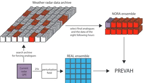
Current radar QPE

select final analogues and the data of the eight following hours

PREVAH Weather radar data archive

NORA ensemble

perturbation field search archive

for forcing analogues REAL ensemble

25x

Fig. 2. Procedure to build the ensembles REAL and NORA. For the REAL ensemble, the current radar QPE is perturbed by a perturba-tion field 25 times to build an ensemble of 25 members. To build the NORA ensemble, a radar data archive is searched to find the situa-tions most similar to the current radar QPE. Then those analogues and the data of the eight hours following each forcing analogue are extracted from the archive, and an ensemble of 12 members with 8 h lead time each is built.

actual potential of NORA in forecasting timing and magni-tude of flash-flood events, but is a trade-off for the compa-rability with the other forecast chains and the computabil-ity in an operational context. For the past events analysed in this study, the whole archive was searched for analogues. This meant that a hindcast of an event could also contain ana-logue situations that actually took place after the considered event in the past. Therefore, the 24 h following the initialisa-tion of each NORA forecast were excluded from the archive in which the analogues were sought. Panziera et al. (2011) found that the results produced in this way did not differ sig-nificantly from results produced when only the hours of the archive preceding the NORA forecasts were included.

2.2.2 REAL – radar ensemble

REAL (Radar Ensemble generator designed for the Alps us-ing LU decomposition) was developed by MeteoSwiss as a probabilistic real-time radar nowcasting tool (zero lead time). It provides an ensemble of 25 members, each of which results from the sum of the current radar image and a stochastic per-turbation field (Fig. 2). This perper-turbation field is a combina-tion of stochastic simulacombina-tion techniques and detailed knowl-edge about the space-time variance and auto-covariance of radar errors (Germann et al., 2009). To obtain this knowl-edge, a suitable network of meteorological ground stations is required. With this methodology the residual space-time un-certainties of the radar precipitation estimates are accounted for. REAL has been produced since May 2007 at hourly in-tervals with a spatial resolution of 2 km×2 km (Germann et al., 2009) for the Lago Maggiore region in the southern Swiss Alps (Fig. 1).

2.2.3 Connection of REAL and COSMO-2

For our study we connected COSMO-2 forecasts to the radar-ensemble nowcasts of REAL. COSMO-2 (C2) is a deterministic numerical weather prediction (NWP) model of the Consortium for Small-scale Modelling (COSMO). It has a lead time of 24 h, a spatial resolution of 2.2 km and has been issued every three hours (00:00, 03:00, 06:00, 09:00, 12:00, 15:00, 18:00, 21:00 UTC) since the beginning of demonstration period of MAP D-PHASE (Rotach et al., 2009) in June 2007. The connection with REAL implies that COSMO-2 meteorological input is actually propagated through the hydrological model every hour with 25 differ-ent initial conditions stemming from the nowcast obtained by forcing PREVAH with REAL.

2.2.4 Deterministic forecasts

In addition to the two ensemble forecast chains with NORA and REAL-C2, we also tested the performance of two deter-ministic model chains. They are constructed like the REAL-C2 forecasts, but unlike with REAL, the initial conditions are derived by driving PREVAH with the deterministic weather radar QPE (RADAR) or interpolated rain-gauge data (PLU-VIO). The data for the interpolated precipitation surfaces originated from automated rain-gauge stations, which have a temporal resolution of 15 to 30 min. These were aggre-gated to hourly values and interpolated with inverse distance weighting over the areas of the test catchments on a 500 m

×500-m grid. Additionally, a bias correction factor was de-termined by calibration (Zappa and Kan, 2007) and applied to all interpolated values, in order to minimise the total dis-charge volume error at the catchment outlets (Viviroli et al., 2009a). The radar QPE was taken from the weather radar on Monte Lema (Fig. 1). They are available at a temporal res-olution of five minutes and at a spatial resres-olution of 1 km2, but were aggregated to hourly time steps and downscaled to a 500 m×500-m grid.

COSMO-2 takes 2.5 h to assimilate, compute and dissem-inate. Since COSMO-2 is produced every three hours, this means that the COSMO-2 forecast is three to five hours old by the time it can be used for the hydrological forecast.

Table 1 shows the schedule for connecting COSMO-2 forecasts to nowcasts forced by REAL, RADAR or PLUVIO.

2.2.5 Study period

Table 1. COSMO-2 forecasts connected to discharge nowcasts forced by REAL, deterministic radar QPE (RAD) and interpolated rain-gauge data (PLU). Times are in hours UTC.

Initialisation of Start of

COSMO-2 forecast Available at discharge forecast

00:00 02:30 03:00, 04:00, 05:00

03:00 05:30 06:00, 07:00, 08:00

06:00 08:30 09:00, 10:00, 11:00

09:00 11:30 12:00, 13:00, 14:00

12:00 14:30 15:00, 16:00, 17:00

15:00 17:30 18:00, 19:00, 20:00

18:00 20:30 21:00, 22:00, 23:00

21:00 23:30 00:00, 01:00, 02:00

distributed over 40 events. We analysed all 1389 forecasts, each of which consists of eight hours, for all forecasting chains included in our study. The 40 individual events are plotted sequentially in Fig. 3 for the Verzasca Catchment, as an example, along with the NORA and REAL-C2 forecasts for 3 and 6 h lead time.

2.3 The catchments

Catchments were selected in the Lago Maggiore region in southern Switzerland, where NORA and REAL are avail-able. Until today these two products have been specially pro-duced for research purposes and are therefore only available for this limited region (Fig. 1). In many catchments in the re-gion, water is intensively managed for hydropower produc-tion. We therefore selected two smaller catchments which are not, or only slightly, affected by water management, as well as a large catchment to explore the effects of scale.

The Calancasca Catchment is 120 km2 and the smallest of the three catchments. The Calancasca valley is a sub-catchment of the Ticino sub-catchment, and is very rural and mountainous with steep slopes ranging from 740 m a.s.l. to 3200 m a.s.l. in altitude. At the top of the catchment a small glacier is covering 1.1 % of the catchment area. The catch-ment is little affected by hydropower, but some of the head-water is partly redirected to a hydropower plant in the neigh-bouring catchment to the east. This diversion is taken into account in the hydrological model with the routing module. Downstream of the Calancasca gauge, the stream water is stored in a small retention lake for hydropower production.

The Verzasca Catchment is 186 km2in area ranging from 490 to 2900 m a.s.l. It is very little influenced by human ac-tivity. At altitudes above the discharge gauge in Lavertezzo it is not affected by any water management but below the gauge, the river Verzasca flows into Lago di Vogorno, a reten-tion lake for hydropower producreten-tion. The basin is the main focus area for our research group. Wöhling et al. (2006) presented the results of model calibration and introduced an assimilation procedure aimed at improving the quality

of initial conditions prior to and during an event. Zappa et al. (2011) developed and tested a methodology to quan-tify the relative contribution of different sources of uncer-tainty (forcing, initial conditions and model parameter esti-mation) to the total uncertainty of a real-time flood forecast. Germann et al. (2009) and Liechti et al. (2013) focused on the verification of the use of REAL as a forcing for real-time nowcasts. The present study is an incremental contribution, that goes beyond nowcasting. The connection of nowcasts with COSMO-2 and the novel radar-based ensemble fore-cast NORA allow us to investigate flash-flood forefore-casts with some hours lead time.

The Ticino catchment is 1515 km2in area. It is much more densely populated and thus more influenced by human activ-ity than the two small catchments. The main valley of the Ticino catchment is part of one of the main transit routes that crosses the Alps. Hence the lower area of the catchment, where the valley is broad enough, is intensively used for in-dustry and agriculture, whereas the steep slopes are only little used. Altitudes range from 220 m to 3400 m a.s.l. The influ-ence of water management is substantial, but all water re-mains in the catchment and reaches the gauge in Bellinzona. 2.4 Experimental set-up

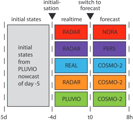
Our experimental set-up in hindcast mode for the five dif-ferent forecasting chains consisted of a nowcasting part with zero lead time (realtime) and a forecasting part (Fig. 4). The nowcasting part was initialised five days prior to the onset of the NORA forecast (t0) by the model state derived from a reference run forced by pluviometer data (Fig. 4). This real-time part was run for four days, which meant the influences of the initial model state are reduced at the start of the fore-casting part at time t0. The five forefore-casting chains analysed are

1. NORA: NORA forecast initialised by a deterministic RADAR nowcast.

2. PERS: the persistence of the current radar QPE at time t0 (i.e. taking the signal of t0 for the next eight hours) initialised by a deterministic RADAR nowcast. 3. REAL-C2: COSMO-2 forecast initialised by a

proba-bilistic REAL nowcast.

4. RAD-C2: COSMO-2 initialised by a deterministic RADAR nowcast.

5. PLU-C2: COSMO-2 initialised by a deterministic PLUVIO nowcast.

Fig. 3. NORA and REAL-C2 discharge ensemble for the Verzasca River for all 40 events in the study period. The panels (a) and (c) show the discharge ensembles at 3 h lead time, and the panels (b) and (d) show the discharge ensembles at 6 h lead time. The individual events are separated by dashed vertical lines. The dates given in thexaxis refer to the date of the beginning of each event.

1. NORA vs. RAD-C2, showing the effect of ensemble forcing.

2. REAL-C2 vs. RAD-C2, showing the effect of an en-semble of initial conditions.

3. NORA vs. REAL-C2, setting the two ensemble fore-casting chains in relation to each other.

The comparison of PERS with the other forecast chains shows if there is actually any benefit in producing a fore-cast. The PLU-C2 forecasting chain stands for itself and has

to be seen as a reference. Compared to the radar-based fore-casting chains this chain has an advantage due to the fact that the hydrological model was calibrated using rain-gauge data. The diagram in Fig. 4 visually explains the different model chains and introduces the names and the colour scheme used from now on for the different forecasting chains.

2.5 Verification methods

8h t0

-4d -5d

RADAR

REAL

RADAR

PLUVIO

COSMO-2 COSMO-2

PERS

COSMO-2 initial

states from PLUVIO nowcast of day -5

initial states realtime forecast

initiali-sation switch to forecast

RADAR NORA

Fig. 4. Diagram showing the different forecasting chains. From the top: NORA, PERS, REAL-C2, RAD-C2 and PLU-C2.

performance of the different forecasting chains for each lead time (1–8 h) separately, as well as for six different thresholds with the following measures of skill:

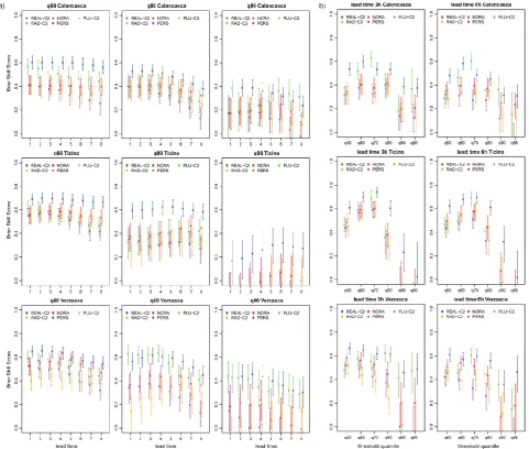
The Brier skill score (BSS) is an ideal measure to compare the performance of probabilistic and deterministic forecasts (Wilks, 2006). The BSS is based on the Brier Score (BS), which describes the quality of the forecast system in predict-ing the probability to exceed a predefined threshold by mea-suring the squared probability error. A perfect forecast sys-tem would have a BS of zero. In order to compare the differ-ent forecast systems to each other, we made use of the BSS, which sets the skill of the different forecasts in relation to a reference forecast. A perfect forecast has a BSS of 1, whereas forecasts worse than the reference forecast have a skill below 0. In our study, the reference forecast was the probability of exceedance for the predefined thresholds based on the sam-ple climatology. The samsam-ple incorporated all discharge ob-servations from hours covered by one or more NORA fore-casts. This resulted in a sample size of 1788 h. The thresh-olds analysed in our study correspond to the 0.5, 0.6, 0.7, 0.8, 0.9 and 0.95 quantile of the sample climatology, which we refer to as q50, q60, q70, q80, q90 and q95. As the sam-ple is restricted to the hours covered by NORA, the actual values of the thresholds quantiles are higher than the ones used in our previous study (Liechti et al., 2013). To esti-mate the uncertainty of the BSS values, we applied the boot-strapping method (Efron, 1992). Thus 500 random samples of forecast-observation pairs were drawn with replacement from the 1389 h belonging to each lead time leading to the confidence limits (95 %) shown in Fig. 5.

The False Alarm Ratio (FAR) and Probability Of Detection (POD) are interlinked and therefore shown together. Both are

measures to evaluate deterministic predictions, where the en-sembles were reduced to their medians. FAR is the fraction of the forecast threshold exceedances that turn out to be wrong. The best FAR value is zero, which means that each positive forecast was followed by a threshold exceedance. POD is the ratio of correctly forecast threshold exceedances to the num-ber of times the event really happened. The best POD value is one, which means that each observed threshold exceedance was forecast. The POD is only sensitive to missed events and not to false alarms, and thus can always be improved by fore-casting an event more frequently. This would, however, lead directly to an increase in false alarms and would, for extreme events, result in an overforecasting bias (Bartholmes et al., 2009; Wilks, 2006).

The ROC area (ROCA) is the area under the ROC (rela-tive operating characteristic) curve. A ROC curve is drawn in a ROC diagram, which incorporates information on the POD (yaxis) and the false alarm rate (xaxis) for the whole range of forecast probabilities. The false alarm rate is the frac-tion of non-occurrences for which a threshold exceedance was forecast. A perfect forecast will result in a ROC curve connecting the points (0/0), (0,1) and (1/1) of the ROC di-agram. An unskilful forecast will not lie above the diago-nal (0/0),(1,1). Thus the area under the ROC curve is a con-venient way to express the degree of discrimination. ROC is not, however, sensitive to an overall bias, which means that ROC actually indicates the potential skill that would be achieved if the forecasts were correctly calibrated (Wilks, 2006). Therefore we also show the bias of the different fore-casting chains.

3 Results

First we show how the spread of the two ensembles NORA and REAL-C2 generally develops over lead time. We then present the results for the three catchments separately. The results of the analysis with ROC area are summarised for all catchments together. Finally, we present a forecast for the Calancasca as it appears in operational mode.

3.1 Chained time series

Fig. 5. (a) Brier skill score (BSS) according to lead time for the threshold quantile q60, q80 and q90. (b) BSS according to the threshold quantiles q50 to q95 for 3 and 6 h lead time. Error bars indicate the 95 % confidence limits around the estimated BSS value. Positive BSS values indicate an improvement in the forecast over the reference forecast, which in this case is the sample climatology.

and Calancasca catchments the spread of REAL-C2 is larger than that of NORA for all lead times, although for Calan-casca the difference is relatively small from 6 h lead time on. For Verzasca, the spread of REAL-C2 is only larger than that of NORA for up to 4 h lead time, and from 6 h lead time on-wards NORA forecasts have a larger spread than REAL-C2 forecasts.

3.2 Calancasca

BSS values for REAL-C2 generally decrease with increas-ing threshold and longer lead times. REAL-C2 shows skill on all thresholds and all lead times. The highest BSS values are reached with q60 (0.56–0.6), but for q90 and q95 BSS values are still as high as 0.35 to 0.4 (Fig. 5b). NORA shows

0.0 0.2 0.4 0.6 0.8 1.0

Calancasca lead time 3h

threshold quantile q50 q60 q70 q80 q90 q95

● ● ● ● ● ● ● ● ● ● ● ● ● ● ● ● ● ● ● ● ● ● ● ● ● ● ● ● ● ● ● ● ● ● ● ● ● ● ● ● ● ● ● ● ● ● ● ● ● ● ● ● ● ● ● ● ● ● ● ● ● ● PLU−C2 PERS NORA RAD−C2 REAL−C2 FAR POD 0.0 0.2 0.4 0.6 0.8 1.0

Calancasca lead time 6h

threshold quantile q50 q60 q70 q80 q90 q95

● ● ● ● ● ● ● ● ● ● ● ● ● ● ● ● ● ● ● ● ● ● ● ● ● ● ● ● ● ● ● ● ● ● ● ● ● ● ● ● ● ● ● ● ● ● ● ● ● ● ● ● ● ● ● ● ● ● ● ● ● ● PLU−C2 PERS NORA RAD−C2 REAL−C2 FAR POD 0.0 0.2 0.4 0.6 0.8 1.0

Ticino lead time 3h

threshold quantile q50 q60 q70 q80 q90 q95

● ● ● ● ● ● ● ● ● ● ● ● ● ● ● ● ● ● ● ● ● ● ● ● ● ● ● ● ● ● ● ● ● ● ● ● ● ● ● ● ● ● ● ● ● ● ● ● ● ● ● ● ● ● ● ● ● ● ● ● ● ● PLU−C2 PERS NORA RAD−C2 REAL−C2 FAR POD 0.0 0.2 0.4 0.6 0.8 1.0

Ticino lead time 6h

threshold quantile q50 q60 q70 q80 q90 q95

● ● ● ● ● ● ● ● ● ● ● ● ● ● ● ● ● ● ● ● ● ● ● ● ● ● ● ● ● ● ● ● ● ● ● ● ● ● ● ● ● ● ● ● ● ● ● ● ● ● ● ● ● ● ● ● ● ● ● ● ● ● PLU−C2 PERS NORA RAD−C2 REAL−C2 FAR POD 0.0 0.2 0.4 0.6 0.8 1.0

Verzasca lead time 3h

threshold quantile q50 q60 q70 q80 q90 q95

● ● ● ● ● ● ● ● ● ● ● ● ● ● ● ● ● ● ● ● ● ● ● ● ● ● ● ● ● ● ● ● ● ● ● ● ● ● ● ● ● ● ● ● ● ● ● ● ● ● ● ● ● ● ● ● ● ● ● ● ● ● PLU−C2 PERS NORA RAD−C2 REAL−C2 FAR POD 0.0 0.2 0.4 0.6 0.8 1.0

Verzasca lead time 6h

threshold quantile q50 q60 q70 q80 q90 q95

● ● ● ● ● ● ● ● ● ● ● ● ● ● ● ● ● ● ● ● ● ● ● ● ● ● ● ● ● ● ● ● ● ● ● ● ● ● ● ● ● ● ● ● ● ● ● ● ● ● ● ● ● ● ● ● ● ● ● ● ● ● PLU−C2 PERS NORA RAD−C2 REAL−C2 FAR POD 0.5 1.0 1.5 2.0

Calancasca lead time 3h

threshold quantile

frequnecy bias

q50 q60 q70 q80 q90 q95

● ● ● ● ● ● ● ● ● ● ● ● ● ● ● ● ● ● ● ● ● ● ● ● ● ● ● ● ● ● PLU−C2 PERS NORA RAD−C2 REAL−C2 0.5 1.0 1.5 2.0

Calancasca lead time 6h

threshold quantile

frequnecy bias

q50 q60 q70 q80 q90 q95

● ● ● ● ● ● ● ● ● ● ● ● ● ● ● ● ● ● ● ● ● ● ● ● ● ● ● ● ● ● PLU−C2 PERS NORA RAD−C2 REAL−C2 0.5 1.0 1.5 2.0

Ticino lead time 3h

threshold quantile

frequnecy bias

q50 q60 q70 q80 q90 q95

● ● ● ● ● ● ● ● ● ● ● ● ● ● ● ● ● ● ● ● ● ● ● ● ● ● ● ● ● ● PLU−C2 PERS NORA RAD−C2 REAL−C2 0.5 1.0 1.5 2.0

Ticino lead time 6h

threshold quantile

frequnecy bias

q50 q60 q70 q80 q90 q95

● ● ● ● ● ● ● ● ● ● ● ● ● ● ● ● ● ● ● ● ● ● ● ● ● ● ● ● ● ● PLU−C2 PERS NORA RAD−C2 REAL−C2 0.5 1.0 1.5 2.0

Verzasca lead time 3h

threshold quantile

frequnecy bias

q50 q60 q70 q80 q90 q95

● ● ● ● ● ● ● ● ● ● ● ● ● ● ● ● ● ● ● ● ● ● ● ● ● ● ● ● ● ● PLU−C2 PERS NORA RAD−C2 REAL−C2 0.5 1.0 1.5 2.0

Verzasca lead time 6h

threshold quantile

frequnecy bias

q50 q60 q70 q80 q90 q95

● ● ● ● ● ● ● ● ● ● ● ● ● ● ● ● ● ● ● ● ● ● ● ● ● ● ● ● ● ● PLU−C2 PERS NORA RAD−C2 REAL−C2

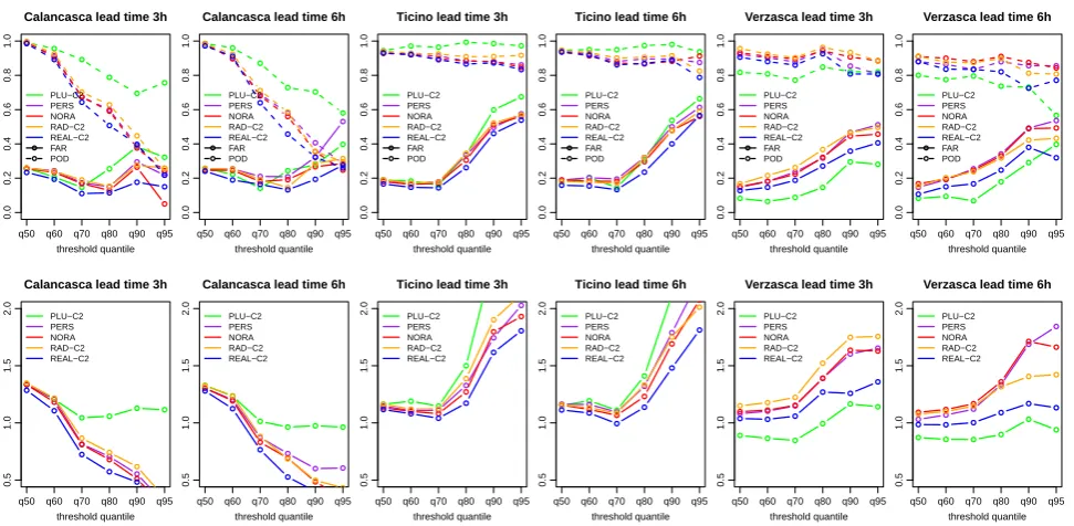
Fig. 6. Probability of detection (POD, dashed line), false alarm ratio (FAR, solid line) and BIAS (lower panel) for each catchment for the thresholds q50 to q95 with 3 and 6 h lead time. Best FAR equals 0, best POD and BIAS equals 1.

all other forecast chains on this threshold. For the highest quantile PLU-C2 also shows skill over all lead times, vary-ing between 0.14 and 0.36.

The probability of detection (POD) for PLU-C2 is higher than for the other forecast chains, as are the FAR values for thresholds q80 to q95 (Fig. 6). POD and FAR for PLU-C2 be-have symmetrically from q70 to q95, which is not the case for the other forecast chains. POD for REAL-C2, NORA, PERS and RAD-C2 rapidly decrease above q60. FAR are lowest for REAL-C2 on all quantiles except q95. FAR and POD for NORA, PERS and RAD-C2 are about the same. FAR values range between 0.1 and 0.3 and POD values drop from 0.9 at q60 to 0.2–0.3 at q95. If we increase the lead time from 3 to 6 h, the main difference is with the q95 threshold, where the FAR values are highest for all forecasting chains (Fig. 6). The different behaviour of the different forecasting chains is also mirrored in the bias. Forecasts for Calancasca have an under-forecasting bias above q60 for all radar-based forecasts. The reasons for that can lie in model calibration but also in the size of the catchment, as for the relatively small Calancasca Catchment errors in the estimation of the location, duration and intensity of predicted rainfall do not smoothen until the catchment outlet. This is most pronounced for REAL-C2. PLU-C2 performs best and is hardly biased above q60. This behaviour does not change with increasing lead time. 3.3 Ticino

REAL-C2 reaches BSS values between 0.6 and 0.75 for thresholds between q50 and q70 for all lead times, but then drop significantly, ranging between 0.2 and 0.3 for q90

times, PERS scores better and on longer lead times RAD-C2 outperforms PERS.

POD values are high for all thresholds and forecast chains, ranging between 0.75 and 0.99. PLU-C2 shows the highest POD, RAD-C2 the second highest and REAL-C2, NORA and PERS about the same scores. FAR values behave differ-ently and increase rapidly after q70 from about 0.15 to 0.55 and 0.7. Again PLU shows the highest FAR, REAL-C2 the lowest and the other forecast chains lie in between on about the same level. This matches with the bias obtained for the forecasts in the Ticino catchment. The bias is about 1–1.2 for q50 to q70, and then increases rapidly for all forecasting chains. PLU-C2 is the most biased and REAL-C2 the least over all thresholds. The same behaviour for bias, POD and FAR can be seen when looking at longer lead times, although the POD values for RAD-C2 on q95 are an exception as they are below those for NORA and PERS, and lower than at 3 h lead time.

The forecast chains are ranked in the same order for Ticino and Calancasca for POD and FAR, but the actual values of POD and FAR behave reversed, which is also mirrored in the overforecasting bias for the Ticino catchment. The reason for this overforecasting bias as well as for the increasing BSS with lead time is most probably the water management in the catchment, which causes that the rainfall of a storm does not reach the catchment outlet in the estimated time, but is stored or redirected and delayed.

3.4 Verzasca

Up to q80 BSS values for REAL-C2 are around 0.6, while for q90 and q95 they are between 0.4 and 0.5. The values gen-erally decrease with increasing lead time. Values for NORA are lower than for REAL, and for q60 and q70, values range between 0.45 and 0.6 with a maximum at 4 and 5 h lead time. BSS values for q80 are around 0.4 with a maximum at lead time 3 (Fig. 5a). For q90 and q95, BSS values are around 0.2 up to lead times 5 and 6, but then decrease rapidly towards no skill. The persistence (PERS) starts from the same level as with NORA on the shortest lead times (BSS 0.55). How-ever, the skill decreases with increasing threshold (Fig. 5b), and the decrease in BSS over lead time is faster for higher thresholds (Fig. 5a). BSS values for RAD-C2 decrease from 0.5 on q50 to 0.3–0.4 on q70. The BSS for short lead times on q80 are very low, but increase to a maximum of 0.35 for 5 h lead time. Similar to the persistence, q90 and q95 have no skill on the shortest lead times, however, BSS values show some skill for longer lead times. PLU-C2 reaches BSS values of around 0.6 for q60 to q80, which decrease with lead time (Fig. 5a). The highest BSS value for the shorter lead times (1–4 h) was reached with q80 (0.63). For the high thresholds, q90 and q95, BSS values still ranged between 0.4 and 0.5 for lead times of 1 to 3 h. If the radar products are compared, scores for NORA are generally below those for REAL, but above those of RAD-C2. For lead times 1 and

2, PERS outperforms RAD-C2 on high thresholds. However, for longer lead times RAD-C2 performs better than PERS. Comparing NORA with PLU-C2, we see that for q50 NORA still scores significantly higher than PLU-C2. This changes for q60 lead time 4, and from q70 onwards PLU-C2 shows better skill than NORA. This difference is most pronounced for short lead times.

All forecast chains show POD values above 0.8 on all thresholds. However, POD and also FAR values for PLU-C2 behave differently in the Verzasca Catchment than in the other two catchments. For Verzasca, PLU-C2 shows the low-est FAR and POD values of all forecast chains except q90 and q95, where REAL-C2 is a little bit lower in POD. FAR values generally increase with increasing threshold from about 0.15 to 0.4/0.5. REAL-C2 was the radar product that performed best. With increasing lead time, NORA outperforms RAD-C2 in POD. However, NORA also shows higher FAR values on thresholds higher than q60. Furthermore, for longer lead times, PLU-C2 reaches the lowest POD and highest FAR on q95 and not on q90, unlike for shorter lead times. Radar-based forecasting chains show a significant overforecasting bias for q80 to q95, which is most probably a calibration is-sue. PLU-C2 slightly underforecasts up to q70, and slightly overforecasts for q90 and q95. With increasing lead time, the bias for RAD-C2 becomes smaller for the high thresholds.

3.5 ROC area

The ROC areas presented in Tables 2–4 are generally higher than 0.7, which is considered to be the minimum value for a forecast system to be useful for a decision maker (Buizza et al., 1999). For Ticino and Verzasca, they do not drop be-low 0.9 up to q90. For Calancasca they are a bit be-lower, es-pecially for NORA and for the high thresholds. For Calan-casca and Ticino, the REAL-C2 forecasts have higher ROC areas than NORA forecasts on all lead times and thresh-olds, although this difference decreases with increasing lead time. For the Verzasca Catchment, the advantage of REAL-C2 over NORA is only clearly evident on short lead times. ROC areas for REAL-C2 decrease with lead time (except Ti-cino, q90), but this is not the case for NORA forecasts.

3.6 Forecast as in operational mode

Table 2. ROC area for NORA and REAL-C2 forecasts of the Calan-casca Catchment, with lead times 03:00, 06:00 and 08:00, for the threshold quantiles q60 to q95.

Calancasca

lt3 lt6 lt8

nora real nora real nora real

q60 0.874 0.935 0.877 0.929 0.879 0.924

q70 0.826 0.937 0.853 0.919 0.85 0.899

q80 0.817 0.945 0.839 0.923 0.826 0.899

q90 0.723 0.887 0.764 0.876 0.733 0.830

q95 0.652 0.897 0.736 0.838 0.725 0.825

Table 3. ROC area for NORA and REAL-C2 forecasts of the Ticino catchment, with lead times 03:00, 06:00 and 08:00, for the threshold quantiles q60 to q95.

Ticino

lt3 lt6 lt8

nora real nora real nora real

q60 0.911 0.962 0.913 0.959 0.914 0.958

q70 0.920 0.977 0.911 0.960 0.905 0.950

q80 0.902 0.968 0.914 0.967 0.917 0.955

q90 0.905 0.949 0.915 0.951 0.896 0.947

q95 0.934 0.971 0.944 0.968 0.925 0.946

Table 4. ROC area for NORA and REAL-C2 forecasts of the Verza-sca Catchment, with lead times 03:00, 06:00 and 08:00, for the threshold quantiles q60 to q95.

Verzasca

lt3 lt6 lt8

nora real nora real nora real

q60 0.918 0.95 0.915 0.933 0.895 0.918

q70 0.916 0.954 0.923 0.935 0.904 0.911

q80 0.941 0.973 0.939 0.946 0.918 0.910

q90 0.934 0.967 0.911 0.922 0.887 0.888

q95 0.954 0.985 0.942 0.940 0.918 0.927

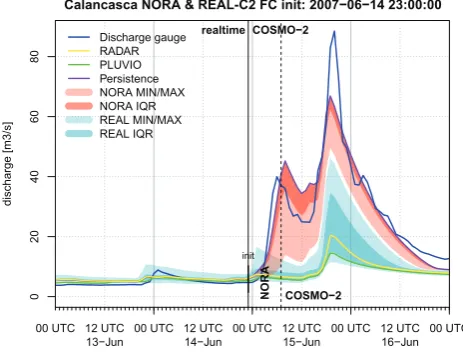
peak, which occurred seven hours after the forecast initialisa-tion (t0), but underestimates the main peak, which occurred 21 h after t0. The REAL-C2 forecast misses this first peak and also underestimates the second peak. For the forecast initialised during the event, however, NORA still underes-timates the main peak, but REAL-C2 captures it.

4 Discussion

The skills of the different forecast chains, are easier to com-pare for lower thresholds as the results are clearer and more persistent over the catchments and lead times. Thus general conclusions about the performance of NORA and the other

Discharge gauge RADAR PLUVIO Persistence NORA MIN/MAX NORA IQR REAL MIN/MAX REAL IQR

00 UTC 12 UTC 00 UTC 12 UTC 00 UTC 12 UTC 00 UTC 12 UTC 00 UTC

13−Jun 14−Jun 15−Jun 16−Jun

init

NORA COSMO−2 realtime COSMO−2

Calancasca NORA & REAL-C2 FC init: 2007−06−14 23:00:00

0

20

40

60

80

discharge [m3/s]

Fig. 7. Forecast simulation for the Calancasca initialised on 14 June 2007 at 23:00. At the time of the initialisation of NORA (vertical solid line), the nowcasts driven by REAL, RADAR and PLUVIO were connected to COSMO-2. After eight hours (vertical dashed line), NORA was also connected to COSMO-2. The analy-sis covers the eight hours covered by NORA forecasts, that is, the time frame between the vertical solid and dashed lines in the graph above.

forecasting chains can only be made for threshold quantiles up to q80. For higher quantiles the results vary considerably between the three catchments included in the study.

00 UTC 12 UTC 00 UTC 12 UTC 00 UTC 12 UTC 00 UTC 12 UTC 00 UTC 13−Jun 14−Jun 15−Jun 16−Jun

0

20

40

60

80

100

discharge [m3/s]

Discharge gauge RADAR PLUVIO Persistence NORA MIN/MAX NORA IQR REAL MIN/MAX REAL IQR

init

NORA COSMO−2

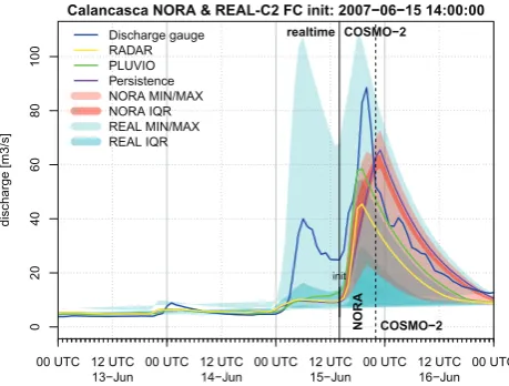
realtime COSMO−2

Calancasca NORA & REAL-C2 FC init: 2007−06−15 14:00:00

Fig. 8. Forecast simulation for the Calancasca initialised on 15 June at 14:00. For a description, see Fig. 7.

during the nowcast part performs better than PERS. As the spread already develops during the nowcast period the ad-vantage of the ensemble approach comes into effect already at the very start of the forecast period.

Thus, despite the difficulties involved with weather radar estimates in an alpine region, producing these computation-ally expensive radar-based ensemble forecasts pays off, as the skill of the hydrological forecast is improved already from the start of the forecast period and stays higher also for longer lead times.

4.1 Effect of ensemble forcing: NORA vs. RAD-C2

Panziera et al. (2011) also compared the performance of NORA with the performance of COSMO-2 for the same rain-fall thresholds. For light rainrain-fall (threshold > 0.5 mm h−1), they found NORA to be better than COSMO-2 for 1–2 h lead times, and for the higher threshold (3 mm h−1)NORA out-performed COSMO-2 up to a lead time of 3–4 h. In the corre-sponding experiment in our study, we compared NORA with RAD-C2, and found that for thresholds up to q80, NORA generally performs better than RAD-C2 for all lead times, except for Calancasca on lead times 4 to 5 h. For the Ticino and Calancasca catchments, the 95 % interval of the boot-strapped BSS values of NORA and RAD-C2 overlap quite a lot (Fig. 5a), but a Student’s t test on a 5 % significance level showed that BSS values of RAD-C2 and NORA are all different apart from Ticino q70 with lead times 4h and 5 h, q90 lead time 7 h and Calancasca q60 lead time 3 h. The ad-vantage of NORA over RAD-C2 up to q80 is, however, clear for the Verzasca Basin. For the highest quantiles (q90 and q95), the results differ between the catchments. However, for the Calancasca NORA significantly outperforms RAD-C2 from 4 h lead time onwards. For Verzasca, on the other hand, NORA performs better than RAD-C2 up to 5 to 7 h. Forecasts for Ticino basically show no skill on the highest

quantile, except NORA on q90, but the BSS values are very small, probably because of the general overforecasting on these high quantiles as the catchment is influenced heavily by water management. It should be noted that the uncertainty of the results for forecast performances is larger the higher the threshold (Fig. 5b), due to the fact that fewer data points lie over the high thresholds. However, in most cases NORA shows higher scores than RAD-C2, which is indicative of the added value in using an ensemble forcing for the hydrologi-cal modelling.

4.2 Effect of using an ensemble of initial conditions: REAL-C2 vs. RAD-C2

The effect of using an ensemble of initial conditions is shown by the comparison of REAL-C2 and RAD-C2. The differ-ence in forecast performance is a function of the model states after the nowcast period alone, as both forecast chains are forced with the same data during the forecast period. The REAL-C2 forecasting chain performs significantly bet-ter than RAD-C2. The BSS values are higher for all thresh-olds and lead times in all catchments. Furthermore, the 95 % confidence interval of the bootstrapped BSS values is mostly narrower for REAL-C2 and does mostly not overlap with the 95 % confidence interval of the bootstrapped BSS values of RAD-C2. So using an ensemble of initial conditions signifi-cantly improved the forecast skill.

4.3 Radar-based ensemble forecasts: REAL-C2 vs. NORA

REAL-C2 forecasts perform better than NORA forecasts in all three catchments. This suggests that an ensemble of initial conditions is more valuable than an ensemble forecast forc-ing alone. So, for regions where REAL can be produced, that is, in regions where the space-time variance and the auto-covariance of radar errors are known, REAL would be pre-ferred over NORA. REAL also has the advantage that it can be produced continuously and that it is not restricted to oro-graphic precipitation. Nevertheless, NORA can offer a use-ful method to predict near-future discharge in regions where these requirements are not fulfilled, in situations where oro-graphic precipitation (or any other repetitive weather situa-tion) plays a major role in flash-flood triggering and a con-tinuous series of weather radar data is available.

excludes local convective events for computational reasons and because spatially and temporally limited events usually do not result in critical situations (Panziera et al., 2011). This may be correct if the whole Lago Maggiore region is con-sidered, but local convective storms can indeed result in ex-treme discharge events if they remain stationary over a spe-cific catchment.

The advantage of REAL-C2 over NORA is also supported by the ROC areas, which are a measure of the potential skill of the forecasts if the model is correctly calibrated. For the Ticino and Calancasca catchments, the ROC areas for REAL-C2 are always larger than those for NORA. This means that, even if the system has been correctly calibrated with radar data, REAL-C2 would outperform NORA for the current set-up of our study. For the Verzasca Catchment, REAL-C2 seems to perform better than NORA only on short lead times.

4.3.1 Ensemble spread

Regarding the spread, the two ensembles behave as expected over the eight hours analysed. NORA forecasts show an in-creasing spread over lead time. Even though the forcing ana-logues of the NORA ensemble are very similar, the evolution following this initial time step can be very different, and the possibility of divergence between the individual members in-creases with each time step as long as there is still precipita-tion. A NORA forecast also always starts with a single ini-tial state at time t0 (Fig. 4). REAL-C2, on the other hand, is initialised four days prior to the initialisation of NORA, by which time it has already built up some spread. Thus the in-fluence of the initial state is minor after these four days. At time t0 the REAL nowcast is connected with the latest avail-able COSMO-2 forecast. This means that the deterministic COSMO-2 is started with 25 different initial conditions. As the REAL ensemble will have already developed its spread prior to the connection, the change in spread over the fol-lowing eight hours is not as big as for the NORA ensemble, which starts from one single initial state. As soon COSMO-2 stops adding more precipitation the ensemble members con-verge.

The Verzasca is noticeably the only catchment where the spread of the REAL-C2 ensemble decreases with lead time, possibly due to the nature of the events included in the study period. NORA is only produced if the atmospheric condi-tions favour orographic precipitation, which means in the Lago Maggiore region, that the winds are blowing from the southwest or south (Panziera et al., 2011). Thus storms usu-ally move roughly from southwest to northeast, and there-fore arrive and leave the Verzasca Basin earlier than the Ti-cino and Calancasca Basin. This also affects the timing of the discharge peaks of the major events within the study period, and the Verzasca River usually peaks at least one hour ear-lier than the Calancasca River for the events analysed. The Ticino River also peaks after the Verzasca River, but here the

reason is most likely that the Ticino catchment is one order of magnitude bigger than the Verzasca Catchment, and thus reacts more slowly.

The single event in the Calancasca River presented in Figs. 7 and 8 shows that the relatively old COSMO-2 fore-cast available prior to the event, on 14 June 2007 at 23:00, dampens the performance of REAL-C2. COSMO-2 forecasts only little rain for the first about 15 h of our forecast, so that the spread of REAL-C2 does not grow much over the first hours. In such situations NORA can help detect critical sit-uations earlier. However, the comparison with the forecast initialised during the ongoing event suggests that the poten-tial of NORA forecasts mainly lies in the early detection of a coming event rather than in forecasting the magnitude of an event, but more individual events need to be analysed, to be able to draw a general conclusion.

4.4 The reference forecast: PLU-C2

The pluviometer-based forecasts PLU-C2 perform well com-pared to the other forecasting chains, and in some cases even outperform REAL-C2 (Calancasca q70 and q90 at long lead times, Verzasca q80 at short lead times) (Fig. 5). One rea-son for this relatively good performance of the deterministic PLU-C2 is that the hydrological model was calibrated with rain-gauge data, and this calibration is also the basis for all the model chains based on weather radar data. Furthermore, a bias correction factor derived during calibration is applied to all interpolated rain-gauge data. The weather radar data are, however, due to the lack of a homogenous time series long enough to perform a calibration, used without such a correc-tion factor. Thus PLU provides the better initial condicorrec-tions for the COSMO-2 forced forecasts.

Although the PLU-C2 forecasting chain performs gener-ally relatively well, there are quite some differences between the individual catchments. On the highest quantiles q90 and q95, PLU-C2 has no skill in the Ticino catchment, whereas for the Verzasca and Calancasca catchments it is still skilful. This difference for the Ticino catchment can be explained by looking at the bias of PLU-C2 for the Ticino catchment. The PLU-C2 forecasts for Ticino are very positively biased on the highest quantiles. The other forecasting chains also show a positive bias, but not that extreme, as is also indicated by the high FAR combined with still relatively high POD values for high threshold quantiles. Thus extreme events are overfore-casted for the Ticino River, possibly due to the influence of several storage lakes for hydropower production. The precip-itation that actually falls in the catchment is not then recorded at the catchment outlet at the estimated time, but is stored in the lakes.

good performance of PLU-C2 is mostly connected to the fact that PREVAH was calibrated using interpolated rain-gauge data, including a bias correction factor.

5 Conclusions

Our study explored the potential of radar-based ensemble forecasts for flash-flood early warning by comparing two novel radar-based ensemble forecast chains to deterministic forecast products in three catchments of the southern Swiss Alps using the hydrological model system PREVAH. Special emphasis was placed on the added value of the purely radar-based NORA forecasting system. NORA is an analogue-based ensemble forecast for orographic precipitation, con-sisting of 12 members, initialised with the initial conditions derived from a four-day nowcast with deterministic radar QPE. The second ensemble forecasting system evaluated in our study is REAL-C2, where COSMO-2 is initialised with 25 different initial conditions derived from a four-day now-cast with the radar ensemble REAL. Additionally, three de-terministic forecasting chains were analysed. One is the per-sistence of the radar QPE at t0 (PERS), while the other two are COSMO-2 forecasts initialised with initial conditions de-rived from a four-day deterministic nowcast with radar QPEs (RAD-C2) and interpolated rain-gauge data (PLU-C2). We analysed the performance of these five flash-flood forecasting systems for all hours between June 2007 and December 2010 for which NORA forecasts were issued, when triggered by orographic precipitation.

We found a clear preference for the ensemble approach. NORA generally outperformed RAD-C2 for thresholds up to q80. This shows that a radar-based ensemble forcing of the hydrological forecast is superior to a deterministic forc-ing as provided by COSMO-2. Moreover, the better perfor-mance of REAL-C2 over RAD-C2 shows the positive effect of working with an ensemble of initial conditions. Further-more, REAL-C2 performed better than NORA. This com-parison leads to the conclusion that the positive effect of an ensemble of initial conditions is bigger than the positive ef-fect of using a ensemble forecast forcing alone.

A follow-up study may also analyse NORA forecasts with a temporal resolution smaller than one hour. This would po-tentially further enhance the performance in forecasting the timing and magnitude of flash-flood events, and could be beneficial especially for small catchments with very short response time. For computational reasons a simple rainfall-runoff model as proposed by Kirchner (2009) may be con-sidered for this purpose. Future investigations may also use NORA forecasts to derive initial conditions for a subsequent initialisation of NWP forecasts, as in REAL-C2. See the example in Figs. 7 and 8, where COSMO-2 is connected to NORA after eight hours. The ideal time for connecting NORA to COSMO-2 still needs to be decided. According to the results for the Calancasca and Verzasca catchments,

the ideal time for switching from NORA to an NWP fore-cast would probably be after 4 to 5 h. This is also in agree-ment with Panziera et al. (2011) who found that after 4 to 5 h COSMO-2 precipitation forecasts generally perform better than NORA. A connection between REAL and NORA could thus be considered for future work. This would result in an ensemble of 300 members, which would most probably show a very large spread. Thus, to be useful for decision making, some sort of pre-selection of behavioural members would be required. First tests using the Series Distance method (Ehret and Zehe, 2011) to rank REAL members encourage further investigations in this direction. An analysis of this approach would, however, be beyond the scope of the study presented here.

Our study also showed that a well-maintained rain-gauge network is very useful. Nowcasts forced by rain-gauge data provide good initial conditions for subsequent forecasts. Also the rain-gauge data are needed to investigate the space-time variance and auto-covariance of radar errors, which is a prequisite for producing the radar ensemble REAL. For re-gions covered by a rain-gauge network the application of a rain-gauged precipitation ensemble generator as proposed in Rakovec et al. (2012) or Moulin et al. (2009) would be a fur-ther option to account for the uncertainty in the meteorologi-cal input to the hydrologimeteorologi-cal model. Such a rain-gauge-based ensemble could be used, in the same way as REAL was used in our study, to derive an ensemble of initial conditions for a subsequent hydrological forecast forced by NWP data. How-ever, the presented study focused on the use of radar-based ensemble forecasts which are not only restricted to regions covered by a good rain-gauge network. In this respect the calibration of the hydrological model with weather radar data would be most desirable in order to further improve the fore-cast performance. However, this would require a long con-tinuous series of weather radar data.

Generally we can conclude that, if the data required to pro-duce REAL are available, REAL-C2 is the preferred fore-casting chain because it performs better than NORA and is not restricted to events originating from orographic precipita-tion. However, for regions where REAL cannot be produced, NORA might be an option to forecast events triggered by orographic rainfall.

Acknowledgements. We are grateful to MeteoSwiss for permission

to use data from their ground-based and weather radar networks, and to the Swiss Federal Office for Environment for providing us with runoff data from their networks. The authors were fully or partly financed through the EU FP7 Project IMPRINTS (Grant agreement no.: 226555/FP7-843 ENV-2008-1-226555). Special thanks to Felix Fundel for his support with statistics and program-ming and to Silvia Dingwall for language editing. We thank two independent reviewers for their valuable comments on an earlier version of this paper.

References

Addor, N., Jaun, S., Fundel, F., and Zappa, M.: An opera-tional hydrological ensemble prediction system for the city of Zurich (Switzerland): skill, case studies and scenarios, Hy-drol. Earth Syst. Sci., 15, 2327–2347, doi:10.5194/hess-15-2327-2011, 2011.

AghaKouchak, A., Nakhjiri, N., and Habib, E.: An educational model for ensemble streamflow simulation and uncertainty anal-ysis, Hydrol. Earth Syst. Sci., 17, 445–452, doi:10.5194/hess-17-445-2013, 2013.

Ahrens, B. and Jaun, S.: On evaluation of ensemble precipitation forecasts with observation-based ensembles, Adv. Geosci., 10, 139–144, doi:10.5194/adgeo-10-139-2007, 2007.

Alfieri, L., Thielen, J., and Pappenberger, F.: Ensemble

hydro-meteorological simulation for flash flood early de-tection in southern Switzerland, J. Hydrol., 424, 143–153, doi:10.1016/j.jhydrol.2011.12.038, 2012.

Ament, F., Weusthoff, T., and Arpagaus, M.: Evaluation of MAP D-PHASE heavy precipitation alerts in Switzerland during summer 2007, Atmos. Res., 100, 178–189, 2011.

Bartholmes, J. C., Thielen, J., Ramos, M. H., and Gentilini, S.: The european flood alert system EFAS – Part 2: Statistical skill as-sessment of probabilistic and deterministic operational forecasts, Hydrol. Earth Syst. Sci., 13, 141–153, doi:10.5194/hess-13-141-2009, 2009.

Berenguer, M., Corral, C., Sanchez-Diezma, R., and Sempere-Torres, D.: Hydrological validation of a radar-based nowcasting technique, J. Hydrometeorol., 6, 532–549, 2005.

Bowler, N. E., Pierce, C. E., and Seed, A. W.: STEPS: A probabilis-tic precipitation forecasting scheme which merges an extrapola-tion nowcast with downscaled NWP, Q. J. Roy. Meteorol. Soc., 132, 2127–2155, 2006.

Bowler, N. E., Arribas, A., Mylne, K. R., Robertson, K. B., and Beare, S. E.: The MOGREPS short-range ensemble pre-diction system, Q. J. Roy. Meteorol. Soc., 134, 703–722, doi:10.1002/qj.234, 2008.

Buizza, R., Hollingsworth, A., Lalaurette, E., and Ghelli, A.: Probabilistic predictions of precipitation using the ECMWF ensemble prediction system, Weather Forecast., 14, 168–189, doi:10.1175/1520-0434(1999)014<0168:ppoput>2.0.co;2, 1999. Efron, B.: Jackknife-after-Bootstrap Standard Errors and Influence

Functions, J. Roy. Stat. Soc. B Met., 54, 83–127, 1992. Ehret, U. and Zehe, E.: Series distance – an intuitive metric to

quan-tify hydrograph similarity in terms of occurrence, amplitude and timing of hydrological events, Hydrol. Earth Syst. Sci., 15, 877– 896, doi:10.5194/hess-15-877-2011, 2011.

Fundel, F. and Zappa, M.: Hydrological ensemble forecast-ing in mesoscale catchments: Sensitivity to initial conditions and value of reforecasts, Water Resour. Res., 47, W09520, doi:10.1029/2010wr009996, 2011.

Fundel, F., Walser, A., Liniger, M. A., Frei, C., and Appenzeller, C.: Calibrated Precipitation Forecasts for a Limited Area Ensem-ble Forecast System Using Reforecasts, Mon. Weather Rev., 138, 176–189, 2010.

Germann, U. and Zawadzki, I.: Scale-Dependence of the Predictability of Precipitation from Continental Radar Images. Part I: Description of the Methodology, Mon.

Weather Rev., 130, 2859–2873,

doi:10.1175/1520-0493(2002)130<2859:sdotpo>2.0.co;2, 2002.

Germann, U. and Zawadzki, I.: Scale Dependence of the Pre-dictability of Precipitation from Continental Radar Images. Part II: Probability Forecasts, J. Appl. Meteorol., 43, 74–89, doi:10.1175/1520-0450(2004)043<0074:sdotpo>2.0.co;2, 2004. Germann, U., Galli, G., Boscacci, M., and Bolliger, M.: Radar pre-cipitation measurement in a mountainous region, Q. J. Roy. Me-teorol. Soc., 132, 1669–1692, doi:10.1256/qj.05.190, 2006. Germann, U., Berenguer, M., Sempere-Torres, D., and Zappa, M.:

REAL - Ensemble radar precipitation estimation for hydrology in a mountainous region, Q. J. Roy. Meteorol. Soc., 135, 445–456, doi:10.1002/qj.375, 2009.

Gurtz, J., Zappa, M., Jasper, K., Lang, H., Verbunt, M., Badoux, A., and Vitvar, T.: A comparative study in modelling runoff and its components in two mountainous catchments, Hydrol. Process., 17, 297–311, doi:10.1002/hyp.1125, 2003.

Jaun, S. and Ahrens, B.: Evaluation of a probabilistic hydromete-orological forecast system, Hydrol. Earth Syst. Sci., 13, 1031– 1043, doi:10.5194/hess-13-1031-2009, 2009.

Jaun, S., Ahrens, B., Walser, A., Ewen, T., and Schär, C.: A probabilistic view on the August 2005 floods in the upper Rhine catchment, Nat. Hazards Earth Syst. Sci., 8, 281–291, doi:10.5194/nhess-8-281-2008, 2008.

Kirchner, J. W.: Catchments as simple dynamical systems: Catchment characterization, rainfall-runoff modeling, and do-ing hydrology backward, Water Resour. Res., 45, W02429, doi:10.1029/2008wr006912, 2009.

Liechti, K., Zappa, M., Fundel, F., and Germann, U.: Probabilis-tic evaluation of ensemble discharge nowcasts in two nested Alpine basins prone to flash floods, Hydrol. Process., 27, 5–17, doi:10.1002/hyp.9458, 2013.

Mandapaka, P. V., Germann, U., Panziera, L., and Hering, A.: Can Lagrangian Extrapolation of Radar Fields be used for Precipi-tation Nowcasting over Complex Alpine Orography?, Weather Forecast., 27, 28–49, doi:10.1175/waf-d-11-00050.1, 2012. Michelson, D. B.: Systematic correction of precipitation gauge

ob-servations using analyzed meteorological variables, J. Hydrol., 290, 161–177, 2004.

Montani, A., Cesari, D., Marsigli, C., and Paccagnella, T.: Seven years of activity in the field of mesoscale ensemble forecast-ing by the COSMO-LEPS system: main achievements and open challenges, Tellus A, 63, 605–624, doi:10.1111/j.1600-0870.2010.00499.x, 2011.

Morin, E., Jacoby, Y., Navon, S., and Bet-Halachmi, E.: Towards flash-flood prediction in the dry Dead Sea region utilizing radar rainfall information, Adv. Water Resour., 32, 1066–1076, 2009. Moulin, L., Gaume, E., and Obled, C.: Uncertainties on mean areal

precipitation: assessment and impact on streamflow simulations, Hydrol. Earth Syst. Sci., 13, 99–114, doi:10.5194/hess-13-99-2009, 2009.

Panziera, L. and Germann, U.: The relation between airflow and orographic precipitation on the southern side of the Alps as re-vealed by weather radar, Q. J. Roy. Meteorol. Soc., 136, 222– 238, doi:10.1002/qj.544, 2010.

Panziera, L., Germann, U., Gabella, M., and Mandapaka, P. V.: NORA–Nowcasting of Orographic Rainfall by means of Analogues, Q. J. Roy. Meteorol. Soc., 137, 2106–2123, doi:10.1002/qj.878, 2011.

use of a grid-based model for flood forecasting, P. I. Civil Eng.-Wat. M., 165, 65–77, doi:10.1680/wama.2012.165.2.65, 2012a. Price, D., Pilling, C., Robbins, G., Lane, A., Boyce, G., Fenwick,

K., Moore, R. J., Coles, J., Harrison, T., and Van Dijk, M.: Rep-resenting the spatial variability of rainfall for input to the G2G distributed flood forecasting model: operational experience from the Flood Forecasting Centre, in: Weather Radar and Hydrology, IAHS Publication, 532–537, 2012b.

Rakovec, O., Hazenberg, P., Torfs, P. J. J. F., Weerts, A. H., and Ui-jlenhoet, R.: Generating spatial precipitation ensembles: impact of temporal correlation structure, Hydrol. Earth Syst. Sci., 16, 3419–3434, doi:10.5194/hess-16-3419-2012, 2012.

Ranzi, R., Zappa, M., and Bacchi, B.: Hydrological aspects of the Mesoscale Alpine Programme: Findings from field experi-ments and simulations, Q. J. Roy. Meteorol. Soc., 133, 867–880, doi:10.1002/qj.68, 2007.

Rossa, A. M., Laudanna Del Guerra, F., Borga, M., Zanon, F., Set-tin, T., and Leuenberger, D.: Radar-driven high-resolution hydro-meteorological forecasts of the 26 September 2007 Venice flash flood, J. Hydrol., 394, 230–244, 2010.

Rossa, A., Liechti, K., Zappa, M., Bruen, M., Germann, U., Haase, G., Keil, C., and Krahe, P.: The COST 731 Ac-tion: A review on uncertainty propagation in advanced hydro-meteorological forecast systems, Atmos. Res., 100, 150–167, doi:10.1016/j.atmosres.2010.11.016, 2011.

Rotach, M. W., Ambrosetti, P., Ament, F., Appenzeller, C., Arpa-gaus, M., Bauer, H.-S., Behrendt, A., Bouttier, F., Buzzi, A., Corazza, M., Davolio, S., Denhard, M., Dorninger, M., Fontannaz, L., Frick, J., Fundel, F., Germann, U., Gorgas, T., Hegg, C., Hering, A., Keil, C., Liniger, M. A., Marsigli, C., McTaggart-Cowan, R., Montaini, A., Mylne, K., Ranzi, R., Richard, E., Rossa, A., Santos-Muñoz, D., Schär, C., Seity, Y., Staudinger, M., Stoll, M., Volkert, H., Walser, A., Wang, Y., Werhahn, J., Wulfmeyer, V., and Zappa, M.: MAP D-PHASE: Real-Time Demonstration of Weather Forecast Quality in the Alpine Region, B. Am. Meteorol. Soc., 90, 1321–1336, doi:10.1175/2009BAMS2776.1, 2009.

Schellekens, J., Weerts, A. H., Moore, R. J., Pierce, C. E., and Hildon, S.: The use of MOGREPS ensemble rainfall forecasts in operational flood forecasting systems across England and Wales, Adv. Geosci., 29, 77–84, doi:10.5194/adgeo-29-77-2011, 2011. Seed, A. W.: A Dynamic and Spatial Scaling Approach to

Advec-tion Forecasting, J. Appl. Meteorol., 42, 381–388, 2003. Sevruk, B.: Adjustment of tipping-bucket precipitation gauge

mea-surements, Atmos. Res., 42, 237–246, 1996.

Szturc, J., O´sródka, K., Jurczyk, A., and Jelonek, L.: Concept of dealing with uncertainty in radar-based data for hydro-logical purpose, Nat. Hazards Earth Syst. Sci., 8, 267–279, doi:10.5194/nhess-8-267-2008, 2008.

Tobin, C., Nicotina, L., Parlange, M. B., Berne, A., and Rinaldo, A.: Improved interpolation of meteorological forcings for hydrologic applications in a Swiss Alpine region, J. Hydrol., 401, 77–89, 2011.

Velasco-Forero, C. A., Sempere-Torres, D., Cassiraga, E. F., and Gómez-Hernández, J.: A non-parametric automatic blending methodology to estimate rainfall fields from rain gauge and radar data, Adv. Water Resour., 32, 986–1002, 2009.

Villarini, G., Mandapaka, P. V., Krajewski, W. F., and Moore, R. J.: Rainfall and sampling uncertainties: A rain gauge

perspective, J. Geophys. Res.-Atmos., 113, D11102,

doi:10.1029/2007jd009214, 2008.

Viviroli, D., Zappa, M., Gurtz, J., and Weingartner, R.: An introduc-tion to the hydrological modelling system PREVAH and its pre-and post-processing-tools, Environ. Modell. Softw., 24, 1209– 1222, doi:10.1016/j.envsoft.2009.04.001, 2009a.

Viviroli, D., Zappa, M., Schwanbeck, J., Gurtz, J., and Weingart-ner, R.: Continuous simulation for flood estimation in ungauged mesoscale catchments of Switzerland – Part I: Modelling frame-work and calibration results, J. Hydrol., 377, 191–207, 2009b. Werner, M. and Cranston, M.: Understanding the Value of Radar

Rainfall Nowcasts in Flood Forecasting and Warning in Flashy Catchments, Meteorol. Appl., 16, 41–55, 2009.

Weusthoff, T., Ament, F., Arpagaus, M., and Rotach, M. W.: As-sessing the Benefits of Convection-Permitting Models by Neigh-borhood Verification: Examples from MAP D-PHASE, Mon. Weather Rev., 138, 3418–3433, doi:10.1175/2010mwr3380.1, 2010.

Wilks, D. S.: Statistical methods in the atmospheric sciences, 2nd Edn., Elsevier, Amsterdam, 627 pp., 2006.

Wöhling, Th., Lennartz, F., and Zappa, M.: Technical Note: Updat-ing procedure for flood forecastUpdat-ing with conceptual HBV-type models, Hydrol. Earth Syst. Sci., 10, 783–788, doi:10.5194/hess-10-783-2006, 2006.

Zappa, M. and Kan, C.: Extreme heat and runoff extremes in the Swiss Alps, Nat. Hazards Earth Syst. Sci., 7, 375–389, doi:10.5194/nhess-7-375-2007, 2007.

Zappa, M., Rotach, M. W., Arpagaus, M., Dorninger, M., Hegg, C., Montani, A., Ranzi, R., Ament, F., Germann, U., Grossi, G., Jaun, S., Rossa, A., Vogt, S., Walser, A., Wehrhan, J., and Wun-ram, C.: MAP D-PHASE: real-time demonstration of hydrolog-ical ensemble prediction systems, Atmos. Sci. Lett., 9, 80–87, doi:10.1002/asl.183, 2008.