Towards automatic calibration of 2 D flood propagation models

www.hydrol-earth-syst-sci.net/14/911/2010/ doi:10.5194/hess-14-911-2010

© Author(s) 2010. CC Attribution 3.0 License.

Earth System

Sciences

Towards automatic calibration of 2-D flood propagation models

P. Fabio1,2, G. T. Aronica2, and H. Apel3

1_{Dipartimento di Ingegneria Idraulica e Applicazioni Ambientali, Universit`a di Palermo, Palermo, Italy</sub> 2<sub>Dipartimento di Ingegneria Civile, Universit`a di Messina, Messina, Italy}

3_{GFZ German Research Centre for Geoscience, Section 5.4 Hydrology, Potsdam, Germany}

Received: 21 October 2009 – Published in Hydrol. Earth Syst. Sci. Discuss.: 6 November 2009 Revised: 10 March 2010 – Accepted: 20 May 2010 – Published: 7 June 2010

Abstract. Hydraulic models for flood propagation

descrip-tion are an essential tool in many fields and are used, for ex-ample, for flood hazard and risk assessments, evaluation of flood control measures, etc. Nowadays there are many mod-els of different complexity regarding the mathematical foun-dation and spatial dimensions available, and most of them are comparatively easy to operate due to sophisticated tools for model setup and control. However, the calibration of these models is still underdeveloped in contrast to other models like e.g. hydrological models or models used in ecosystem analysis. This has two primary reasons: first, lack of rel-evant data against which the models can be calibrated, be-cause flood events are very rarely monitored due to the dis-turbances inflicted by them and the lack of appropriate mea-suring equipment in place. Second, 2-D models are compu-tationally very demanding and therefore the use of available sophisticated automatic calibration procedures is restricted in many cases. This study takes a well documented flood event in August 2002 at the Mulde River in Germany as an example and investigates the most appropriate calibration strategy for a simplified 2-D hyperbolic finite element model. The model independent optimiser PEST, that enables automatic calibra-tions without changing model code, is used and the model is calibrated against over 380 surveyed maximum water lev-els. The application of the parallel version of the optimiser showed that (a) it is possible to use automatic calibration in combination of 2-D hydraulic model, and (b) equifinality of

Correspondence to: P. Fabio

([email protected])

model parameterisation can also be caused by a too large number of degrees of freedom in the calibration data in con-trast to a too simple model setup. In order to improve model calibration and reduce equifinality, a method was developed to identify calibration data, resp. model setup with likely er-rors that obstruct model calibration.

1 Introduction

Floods are serious events and may have severe socioeco-nomic impacts on vulnerable areas. Thus a reliable evalu-ation of the inundevalu-ation extent and depths of a given flood scenario is a very important support for strategic food risk management. Different models which simulate the hydraulic behaviour of a river system are available and they should be calibrated and tested with care before exploitation.

Model calibration is the process whereby model param-eters are adjusted until a satisfactory match between model response and historical data is achieved. The geometry and the roughness parameters are considered to be the most im-portant elements affecting predicted inundation extent and flow characteristics, as elaborated with wide bibliography by Pappenberger et al. (2005). The roughness parameter will, in part, compensate the sources of errors related to these el-ements (Romanowicz and Beven, 2003; Marks and Bates, 2000), thus the calibration becomes a crucial issue.

912 P. Fabio et al.: Towards automatic calibration of 2-D flood propagation models surface roughness only, but also turbulent momentum losses

not explicitly modelled (Werner et al., 2005a). In addition, roughness coefficients often have to compensate for insuffi-cient model assumption, e.g. depth averaged flow, and model setup, thus becoming what is kown as effective roughness parameters. In general practice, calibration and estimation are performed manually, mostly in a “trial-and-error” fash-ion. This is difficult, complex, subjective, time-consuming and depends much on the expertise of the modellers. How-ever, parameter estimation algorithms can significantly im-prove and facilitate this task, as shown in many other areas of environmental modelling. Here, an objective function that measures the discrepancy between observations and model outputs is defined, and the algorithm adjusts the parameter values to minimise the objective function until a convergence criterion is reached.

In general, automatic calibration procedures can be di-vided in two main families: Global optimisers like the popu-lar population-evolution-based algorithms, such as the Shuf-fled Complex Evolution model developed by the University of Arizona (SCEUA) (Duan et al., 1992, 1993; Sorooshian et al., 1993), and the classical gradient-based approaches, like the Gauss-Levenberg-Marquardt method (Levenberg, 1944; Marquardt, 1963). These optimisation families have pre-viously been mostly been applied to hydrological models, where parameters can be less well defined (i.e. less physi-cally based). Global methods are more robust in finding the global minimum in the parameter space of the objective func-tion but they are computafunc-tionally very demanding. In fact, in order to explore the whole parameter space they require a much higher number of model runs to converge compared to gradient-based methods. Gradient-based methods on the other hand are computational very efficient but the solution can be dependent on the initial parameter values and they might get trapped in a local minimum, if the response space of the objective function is highly complex. However, these methods may be the only possibility to automatically cali-brate CPU time demanding models, like the one presented here. In this case the selection of the initial parameter values has to be taken with care and should be checked by multiple optimisation runs with different starting points, if model run time allows.

In the present study the Gauss-Levenberg-Marquardt method implemented in the parameter estimation tool PEST (acronym for Parameter ESTimation) is used (Doherty, 2004, 2008). PEST is considered the most efficient method com-pared to other gradient based methods (Doherty, 2004, 2008) and it is successfully applied in many scientific fields such as groundwater, hydrological and water quality modelling. While PEST also offers global optimisation routines, this study explores the gradient-based method in a first step for the reasons given above.

Using the gradient-based approach this study focuses on different calibration strategies for a 2-D hydraulic model. It is calibrated against a serious flood event that occurred in

August 2002 on the river Mulde in the city of Eilenburg in Saxony, Germany. In the different calibration strategies four aggregation levels of the spatially distributed surface rough-ness were considered: (a) a single roughrough-ness value for the channel and the whole floodplain; (b) two roughness values attributed to the channel and the whole floodplain; (c) four roughness values attributed to the channel and three land use classes in the floodplain; (d) five roughness values related to the channel and four land use classes in the floodplain.

Being certain that a computer-based model is an imperfect representation of a physical system, a perfect match is not expected from a calibration to the available field measure-ments. This inability may be due to the presence of errors in both data and in the model (Gupta et al., 1998). We assume that the mathematical structure of the model is predetermined and fixed and that the upper and lower bounds of parameter ranges can be specified a priori.

In most cases the calibration of flood inundation models is constraint by insufficient data against which the model can be calibrated. This is especially the case for distributed flood-plain data, causing the often observed dilemma that a spa-tially distributed model is calibrated against bulk flow data in the channel allowing for a high degree of equifinality in model realisations (e.g. Aronica et al., 2002; Bates, 2004; Pappenberger et al., 2005). However, in this study area the flood event occurred in August 2002 was well documented: flood depths were recorded from a large number of water marks, the maximum inundation extent was surveyed from satellite imaging and water marks, and the flood hydrograph was recorded at the upstream flowgauge. This data set en-abled not only the automatic calibration, it will also show that a large amount of data or information do not assure an improvement in the identification of the parameters. It is not only the number, but also the quality of the information con-tained in the data that is important. Increasing the amount of data does not necessarily improve the parameter estimation (Sorooshian et al., 1993). A wide literature analyses simu-lation errors of inundation model discussing of the possible sources in order to obtain acceptable models even at local scale (Bates and De Roo, 2000; Horritt, 2006; Mignot et al., 2006; Schumann et al., 2007; Neal et al., 2009 are just a few examples). In this paper a procedure to remove potentially erroneous data is presented.

2 Methodology

2.1 2-D hydrodynamic model

(DSV), where convective inertial terms are neglected in order to eliminate the related numerical instabilities. The conser-vative mass and momentum equations for 2-D shallow-water flow can be written as

∂H ∂t +

∂p ∂x +

∂q

∂y =0 (1)

∂p ∂t +gh

∂H

∂x +gh Jx=0; ∂q

∂t +gh ∂H

∂y +gh Jy=0 (2) where H(t, x, y) = free surface elevation; p(t, x, y) and q(t,

x, y) =x- andy-components of the unit discharge (per unit width);h= water depth;g= gravitational acceleration; and JxandJy= hydraulic resistances in thex- andy-directions.

The hydraulic resistance is parameterised by the Manning-Strickler formulation, the Manning-Strickler roughness coefficient k (m1/3·s−1) is related to Manning coefficient n (m1/3·s−1) through

k= 1

n, (3)

Equations (1) and (2) were solved by using a finite element technique with triangular elements. The free surface eleva-tion is assumed to be continuous and piece-wise linear inside each element, where the unit discharges in thexandy direc-tions are assumed to be piece-wise constant.

The finite element approach allows a more detailed de-scription of hydraulic behaviour of flow in the flooded ar-eas, in fact unstructured meshes are able to reproduce the complex topography of built-up and urban areas. High hill-top, building blocks, houses and other obstacles are treated as internal islands within the triangular mesh covering the entire flow domain. Being explicitly 2-D the model also al-lows for spatially varying roughness coefficients in the whole model domain. For proper model setup detailed topographic information are required: topographical map preferably with a scale of 1:10 000 and lower, a high spatial resolution DEM and data set about the river topography (a number of cross sections with bed elevations, channel widths and roughness coefficients are useful to improve the mesh descriptive capa-bility in those parts of floodplains; Horritt and Bates, 2001).

2.2 Model calibration

The 2-D model was calibrated using the model independent optimiser PEST (Doherty, 2004, 2008). It gives the possi-bility of an automatic calibration without the necessity to change the model at all, but only the values of the param-eters in one or more model input files. Applying this concept to hydraulic modelling is a step towards a more objective and encompassing model calibration compared to the gen-eral manual practice.

PEST adjusts model parameters to obtain the best match between model generated values and the correspondent mea-surements in a weighted least squared sense. Given the num-ber of degrees of freedom present in the calibration proce-dure of 2-D models, where individual friction parameters

can theoretically be assigned at each computational node and at each time-step (Marks and Bates, 2000) some difficul-ties may arise because of the equifinality problem encoun-tered during the calibration procedure (cf. e.g. Beven, 1993, 1996, 2006; Beven and Binley 1992; see also bibliography in Beven and Freer, 2001).

The parameter estimation software PEST implements the Gauss-Levenberg-Marquardt method (Levenberg, 1944; Marquardt, 1963) for parameter estimation and uncertainty analysis. The method is a combination of gradient descent and Newton’s method. Parameter estimation is an iterative process linearizing the relationship between model parame-ters and model outputs. The linearization is conducted by formulating a Taylor expansion of the actual parameter set. At every iteration the partial derivatives of each model out-put with respect to every parameter are calculated using fi-nite differences. The technique follows the steepest gradient of the objective function until the gradient becomes small with respect to a certain tolerance limit. In the steepest re-gion of the objective function the search for the minimum is performed slowly (with small step size), in shallow regions the movement is quicker (with large steps). Moreover, Mar-quardt improved the method considering each component of the gradient according to the curvature, i.e. the search moves further in the directions in which the gradient is smaller in order to speed up the convergence (this is very important for example when the solution space of the objective function presents a long and narrow valley). The parameter upgrade vector given by the Levenberg-Marquardt method is written as

p−p₀=(Jt·Q·J+λdiag[Jt ·Q·J])−1·Jt ·Q·ε (4) wherep= subsequent parameter vector,p₀= current param-eter values, J = the Jacobian matrix, Q = a diagonal matrix such that the inverse is proportional to the covariance matrix of the observations,λ= the Marquardt lambda.

914 P. Fabio et al.: Towards automatic calibration of 2-D flood propagation models wherem= number of observations;θ= vector of model

pa-rameters (i.e. roughness coefficients);hi,obs= observed

wa-ter depth ati-th site;hisim(θ) = simulated water depth at the

same site generated using the parameter valuesθ.

The aim of PEST is to minimize the Sum of Squares SQ objective functionF (θ )given by

SQ=F (θ)= m X

i=1

wi ·(εi)2 (6)

wherewi are weights that can be assigned to individual ob-servations, resp. errors. The weights in the objective func-tion allow to focus on some observafunc-tions in the optimisafunc-tion, thus, trustworthy observations can have a greater weight than those which cannot be trusted as much. In the present study the unit value has been assigned to all residual weights and the measurements errors have been assumed to be indepen-dent. In fact, it is very difficult to deal with correlations in observed data, especially when there is no a priori informa-tion about them. Under the assumpinforma-tion of independence of the observations, the matrix Q defined in Eq. (4) has diago-nal elements only and the elements of Q are the observation weights.

As already pointed out, the Gauss-Levenberg-Marquardt method is gradient based and uses a local search method to find the minimum of the objective function. It can be criticized because it can be trapped in local objective func-tion minima, so that the solufunc-tion is dependent on the starting point. Global search methods could be used but they require a much greater number of model runs and depending on the particular case of study the cost in terms of time could be-come prohibitive. However, even the number of model eval-uations in gradient based methods in combination with long model run times may also prohibit the application of gradi-ent based methods in many hydraulic model calibrations. For this reason PEST offers a parallel version of the optimiser that considerably decreases the time required for the calibra-tion, if multicore computing facilities are available. Also, the search for the minimum of the objective function using PEST is achieved using fewer model runs than any other parame-ter estimation method (Doherty, 2004, 2008), which favours the usage of PEST additionally. Computational clusters or office grid solution can be used with PEST. However, at present PEST is restricted to Windows-based operation sys-tems, thus the usual Linux-based large computational clus-ters cannot be used unless Windows emulating software is installed. The parallel automatic calibration has been tested in this case study, where a single model runtime was approx-imately 4 h. On a workstation with 8 Intel Xeon X5355 pro-cessors at 2.66 GHz CPU speed, the algorithm converged af-ter 4–9 optimisation iaf-terations, which took 4–5 days for each optimisation run.

After the parameter estimation process PEST calculates the 95% confidence limits of the adjustable parameters if the covariance matrix has been calculated. It should be noted

that parameter confidence limits are calculated on the basis of the same linearity assumption which was used to derive the equations for parameter improvement underlying each PEST optimisation iteration. Moreover no account is taken of pa-rameter upper and lower bounds in the calculation of 95% confidence intervals. For example they are not truncated at the parameter domain boundaries so as not to provide a mis-leading impression of parameter certainty. Thus confidence limits provide only an indication of uncertainty but they are useful to compare different calibration strategies.

2.3 Model performance evaluation

Figure 1 Investigation area overview and topographical map of Eilenburg.

31

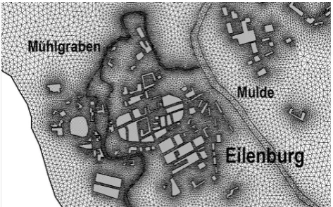
Fig. 1. Investigation area overview and topographical map of

Eilen-burg.

greatly changing the inundation extent and thus the flood area index comparing the simulated and mapped inundation ex-tend. The inappropriateness of the inundation extend for the present case study was already shown in a previous study us-ing different hydraulic models and manual calibration on the event, the model results of estimating the inundation extend were published in Apel et al. (2009). Therefore, in this case more meaningful indexes for the comparison of the differ-ent calibrations are, besides the objective function used in PEST: the mean absolute error (MAE), the root mean square error (RMSE) and the average error (BIAS) of the simula-tion results from the measured maximum inundasimula-tion depths calculated as follows

MAE= 1 m

m X

i=1

|εi|; RMSE= v u u t 1 m

m X

i=1

(εi)2; (7)

BIAS= 1 m

m X

i=1

εi

wherem= number of data points.

3 Case study

The urban area of Eilenburg, located in the federal state of Saxony, Germany, was used in this study. The city is crossed by the Mulde River, a tributary of Elbe, and the M¨uhlgraben bypass, diverted from the main stream approx. 10 km up-stream of Eilenburg (cf. Fig. 1).

In August 2002 a severe flood event hit many European countries along the Elbe and the Danube rivers and many of their tributaries. Germany was affected, and Saxony was German federal state that suffered the most damage. In par-ticular, the city of Eilenburg and the surroundings were com-pletely flooded; inundation depths up to 5 m in the vicinity of the river and 3 m in the town were reached. Because of the severity of the event, the flooding was well documented:

Figure 2. Layout of the mesh of the simplified 2D-finite element model.

32

Fig. 2. Layout of the mesh of the simplified 2-D-finite element

model.

flood depths were surveyed by laser reflectometry of water marks on buildings above ground at 390 points (data pro-vided by Schwarz et al., 2005), thus yielding detailed point information of inundation depths in the town. The accuracy of the laser measurements is in the mm-order. Some higher errors are introduced when the ground reference level was hard to determine, e.g. by bushes growing in front of the building or unclear water marks. No detailed information is available about this, but the errors of the surveyed maximum inundation depths can be assumed at below 0.2 m. The loca-tion of the survey points was determined by handheld GPS. Thus the errors in the location of the survey points are below 6 m. This extensive data set has been used for the calibration of the inundation model.

For the hydraulic model, boundary conditions are always given by the incoming unit flux along the upstream boundary and the water surface elevation at the downstream bound-ary (Aronica et al., 1998b). Upstream boundbound-ary conditions were given by the measured hydrograph at the gauge Golz-ern, which is the closest gauging station and is located on the Mulde approximately 20 km upstream of Eilenburg. The data recorded by the next downstream gauging station of the Mulde River in Bad D¨uben could not be used for model cali-brations, because the water levels largely exceeded the rating curve. Moreover the gauge was also considerably influenced by the floods of the Elbe River, both from overland flow and the nearby junction of the rivers, and it is located at a consid-erable distance to the model domain (about 25 flow km). In the model version used in the calibration normal water depth for the channel and zero water depths for the downstream nodes located in the floodplain have been assumed as lower boundary condition.

916 P. Fabio et al.: Towards automatic calibration of 2-D flood propagation models

Figure 3. Layout of the spatial roughness distribution in the computational domain considered

for the case of study (Woodland 1: deciduous forest, woodland 2: low forest interspersed with

agriculture).

33

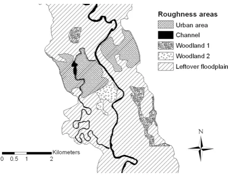
Fig. 3. Layout of the spatial roughness distribution in the

computa-tional domain considered for the case of study (woodland 1: decid-uous forest, woodland 2: low forest interspersed with agriculture).

Cartography (BKG) and is based on topographical maps with a scale of 1:25 000. These maps, especially the elevation in-formation are mainly based on terrestrial surveys supported by remote sensing information in some parts. The errors of the 25 m resolution DEM are estimated by BKG to be below 1m in the flood plains and up to several meters on steep hill-slopes and mountainous areas. Additionally some channel and bank node elevations were taken from channel bathy-metric surveys and linearly interpolated between 18 cross sections available for the model domain. The large railway dam and bridge directly upstream of the town (cf. Fig. 1) are represented in the model, whereas the smaller downstream bridge is not. Channel, floodplain and the extent of the do-main were digitised from the 1:25 000 maps of the area, the length of the modelled reach is about 8.5 km. The reach was restricted to this stretch in order to keep model runtimes at a tolerable level, which are about 4 h for a single model run simulating five days in rhe version used for the calibration study.

The Strickler roughness coefficient is the unique parame-ter involved in the calibration, which is spatially distributed. The model structure allows one coefficient for each triangu-lar element to be used, but based on land use, the domain was divided into five principal regions (Fig. 3). Using the official CORINE land use classification, which is a European stan-dard, four areas were distinguished in the floodplain: the ur-ban area of Eilenburg, two woodlands and the leftover flood-plain. The roughness parameterization was consequently performed on the land use classification.

3.1 Calibration outline

The model calibration was performed against the water depths, not water elevations. It is often argued that

inundation models perform better when calibrated against water elevations than depths. In case of independently de-rived water elevations this may be the cause, because the models can compensate for DEM errors through the rough-ness parameterization. However, we generally argue that cal-ibration against the actual observed variable, the water depth, gives insights into model behaviour and should thus be pre-ferred. Also, in the presented case where no independent ob-servation of water or ground obob-servations are available, the use of water elevations do not improve model performance and calibration. Here the water elevation have to be calcu-lated from the simucalcu-lated, resp. observed inundation depths and the elevation of the underlying DEM. Since PEST opti-mises the model based on the sum of squares that in this case evaluates to the same value (cf. Eq. 5):

εi=hi,obs−hi,sim(θ)=(hi,obs+DEM)−(hi,sim(θ)+DEM)

Different calibration strategies were adopted according to different aggregation levels of the roughness regions. In each region one roughness coefficient has been defined uniformly distributed. In the first level, a single and uniform rough-ness coefficient was adopted for the whole floodplain and the river. In the second level, the river and the floodplain were considered separately. For the third, four roughness areas were considered: the channel and the city areas aggregated in a single region (on the assumption that flow through a mostly paved urban environment, especially with high flow depths as in this case, is similar to open channel flow), the two wood-lands and the leftover floodplain. Finally, the last level con-siders five separate regions according to the CORINE land use distribution shown in Fig. 3.

To overcome the problem of how to choose the range of parameter space, a large range including physical re-alistic values was considered, thus giving space for the estimation of effective parameters. For both main chan-nel and floodplain the lower value for the Strickler rough-ness coefficient was set equal to 5 m1/3·s−1 (equivalent Manning coefficient n is 0.2 m-1/3·s), corresponding to dense wood, and the upper one to 90 m1/3·s−1 (equiva-lent Manning coefficient n is 0.011 m-1/3·s), correspond-ing to concrete. In other studies similar ranges were de-fined: prior ranges used by Werner et al. (2005b) were loosely based on those given by Chow (1959): the range between 0.02 m−1/3·s and 0.1 m−1/3·s for the main chan-nel, and between 0.02 m−1/3·s and 0.3 m−1/3·s for the flood-plain. Pappenberger et al. (2007) adopted a sampling range 0.01–0.2 m−1/3_{·s for the channel and 0.05–0.3 m}−1/3_{·s for}

the floodplain, imposing channel friction always lower than floodplain friction. Bates and Townley (1988) used 0.01– 0.05 m−1/3·s as main channel Manning values, and the con-ditionnfl=3nch+0.01 for the floodplain. Through the utility

Table 1. Different calibration strategies and parameter aggregation used in the study (k= Strickler roughness coefficients).

Calibration Number ofk Aggregated areas Constrains description parameters

A 1 All unconditioned

B 2 Urban area, woodlands roughness of the river always lower and leftover floodplain than roughness of the floodplain as a uniform floodplain

C 2 Urban area, woodlands unconditioned and leftover floodplain

as a uniform floodplain

D 4 Urban area and channel roughness of the river always lower as a single land than roughness of the floodplain use class/roughness area

E 5 All CORINE land use roughness of the river always lower classes than roughness of the floodplain F 5 All CORINE land use unconditioned

classes

roughness of the river to be always lower than the rough-ness of the floodplain. In the context of PAR2PAR this is achieved by defining e.g. for the floodplain a “new” Strickler roughness parameterkfp ratiothat is defined by the ratio of the

Strickler roughness coefficient in the channel to the Strickler roughness coefficient roughness in the floodplain, and im-posing as lower bound of this parameter the unit value: kfp ratio=

kch

kfp

>1 (8)

However, the way PAR2PAR is implemented limits in the definition of parameter bounds, because only bounds for kfp ratiocan be defined, not for the actual parameters

rough-ness parameterskchandkfp. In Table 1 the calibration outline

adopted in the study is summarised.

4 Results and discussion

4.1 Comparison among calibrations

All automatic calibrations performed with PEST converged and successfully improved the objective function. The results in terms of final estimated roughness parameters and confi-dence bounds are collected in Table 2. Initial values were set following criteria suggested by previous experience gained in manual model calibration (Apel et al., 2009). Except for the roughness coefficient related to the channel, each calibration gave quite low Strickler roughness values, i.e. high hydraulic resistance, for the floodplain compared to literature values. Some remarks on this finding can be made. First, roughness values present in literature are usually referred to results of

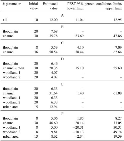
Table 2. Final roughness estimations and confidence bounds for the

calibration scenarios given by PEST. Note: in case of conditioned parameters no confidence bounds can be derived.

kparameter Initial Estimated PEST 95% percent confidence limits value value lower limit upper limit

A

all 10 12.00 11.04 12.95

B

floodplain 20 7.68 – –

channel 30 35.78 23.69 47.86

C

floodplain 8 5.59 4.10 7.09 channel 36 50.54 38.44 62.64

D

floodplain 20 6.46 – –

channel-urban 30 20.35 15.10 25.60

woodland 1 20 4.07 – –

woodland 2 20 4.07 – –

E

floodplain 20 6.33 – –

channel 30 31.64 1.40 61.88

woodland 1 20 6.33 – –

woodland 2 20 6.33 – –

urban area 15 12.94 – –

F

918 P. Fabio et al.: Towards automatic calibration of 2-D flood propagation models

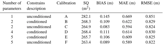
Table 3. Goodness of fit indexes of the different calibration runs using all data points.

Number of Constrains Calibration SQ BIAS (m) MAE (m) RMSE (m) parameters description (m2)

1 unconditioned A 282.1 0.145 0.669 0.851 2 conditioned B 268.3 0.109 0.622 0.829 2 unconditioned C 264.9 0.083 0.594 0.824 4 conditioned D 268.4 0.111 0.614 0.830 5 conditioned E 265.7 0.106 0.609 0.825 5 unconditioned F 263.4 0.089 0.589 0.822

one-dimensional model applications, while in this case study a 2-D model code is applied. Second, usual tabular data are referred to micro-roughness condition that is unrealistic for the floodplain surface. Third, the high roughness may have to compensate for errors introduced by the short reach under study and the lower boundary condition imposed (cf. Sect. 3) in absence of surveyed discharges for the lower boundary, as illustrated in Horritt et al. (2007). Further exploring Ta-ble 2 it is worth noting that the roughness in the river is in some cases very high. This has to attributed to the inten-sity of flood event with large discharge and flow depth over the whole floodplain compared to channel width and depth. In this case the influence of the channel flow on maximum floodplain inundation becomes marginal, because the bulk of the flow is overbank.

When parameters are not conditioned, PEST gives 95%-confidence limits associated to the estimated parameter val-ues. These are statistically derived from the distribution of the parameters during the optimisation. As we can see, the larger the number of involved parameters, the larger become the confidence intervals. Moreover, when the calibration considers five parameters the lower limits are even negative. This does not mean that negative roughness parameters were actually used in the calibration. This is rather the result of the statistical derivation of the confidence limits in case of low mean and high variance, where the lower 95%-confidence bounds can eventually evaluate to negative values. Negative roughness values do not make any sense physically, however, the width of the confidence limits indicate how uncertain the estimation of the parameter is: narrow bands imply higher confidence and thus higher importance of the parameter on the results and vice versa. It also indicates the equifinality of model parameterisations that arise by the increasing number of possible parameter combinations able to match the obser-vation data satisfyingly. Following this rational the inunda-tion depths are dominated by the floodplain area, respectively the floodplain roughness showing the narrowest confidence limits, especially in scenarios C and F. This means that the floodplain surrounding the urban area influence significantly the flow propagation in the urban area. The sensitivity of the model to floodplain roughness is explainable through the

comparatively large extension of that land use class and the fact that it provides the internal boundary conditions for the flow in the urban area.

In case of four conditioned parameters (D), the estimated roughness values for the woodlands fall slightly outside the settled range of parameter space as a result of the condition-ing of the parameters. The utility PAR2PAR required the manipulation of the parameters, so that transformed parame-ters and related bounds are included in the PEST input files, but unfortunately it is very difficult to incorporate and/or con-trol parameter-dependent bounds. Also, the confidence limits are provided for the transformed parameters and not for the roughness parameters of interest.

4.1.1 Model performance

Table 4. BIAS calculated with removed data points for the different calibrations.

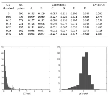
|CV| No. Calibrations CV(BIAS) threshold points A B C D E F

0 390 0.145 0.109 0.083 0.111 0.106 0.089 0.200

0.05 343 0.059 0.018 −0.011 0.020 0.014 −0.006 1.578

0.10 278 0.157 0.112 0.080 0.110 0.105 0.083 0.259 0.15 231 0.128 0.076 0.040 0.079 0.072 0.046 0.425 0.20 192 0.111 0.064 0.031 0.062 0.056 0.034 0.483 0.25 162 0.086 0.041 0.012 0.037 0.033 0.013 0.728

0.30 143 0.066 0.021 −0.011 0.016 0.011 −0.009 1.783

Figure 4. Histograms of absolute coefficient variation and mean of the errors of different

calibration runs for every calibration point.

Fig. 4. Histograms of absolute coefficient variation and mean of the errors of different calibration runs for every calibration point.

calibration data, the usual cause of equifinality. However, the mismatch in this case is just opposite of the normal case: usually a complex model is calibrated with just a few data points, which are often bulk measurements, e.g. a two di-mensional hydraulic model and a downstream discharge hy-drograph. In the present case we deal with many data points, whereas the roughness in the respective land use class is not further distinguished, as well as a fairly coarse DEM. This means we use a comparatively simple model setup which is not sufficient to explain the information content of the cali-bration data properly.

In order to explore the reasons for the equifinality and to possibly reduce it, we take the advantage of the different calibration strategies applied and search for erroneous data points utilizing the different simulation results. We also test whether the calibration is sensitive to a reduced number of calibration points, i.e. an adjustment of data complexity to model complexity. To this end the variance of the residuals of the different calibration results was examined. The idea was to identify and remove calibration points with likely er-rors (DEM, survey, etc.) and then check for sensitivity of the goodness of fit criteria for the calibration runs without run-ning the calibration again in first place. The criterion adopted was the coefficient of variation (CV) of different calibration

runs for every calibration point. The coefficient of variation (CV) is defined as the ratio of the standard deviation to the mean and is a normalized measure of dispersion of a prob-ability distribution, Fig. 4 shows the histograms for the ab-solute value|CV(ε)|and the mean, µ(ε), of the errors for all calibration points of all calibration runs. Based on the CV we defined points as erroneous based on the following ra-tional: points with high mean absolute difference of all cal-ibration runs and low variation (standard deviation) caused by different model parameterization were removed as erro-neous, because they cannot be explained by model param-eterization (or with the current model setup). In terms of CV, these are the points with low CV’s (low standard devi-ation/high mean). Thus points in the calculation with ab-solute coefficients of variation lower than a threshold were removed. For the selection of the threshold, however, no ob-jective measure can be defined. Therefore several thresholds values were selected:|CV|=0, 0.05, 0.1, 0.15, 0.2, 0.25 and 0.3. After simply removing points with|CV|less than each threshold the BIAS for every calibration was computed again with the current calibrated model results (Table 4). Inspect-ing Table 4 it is possible to identify two particular thresholds (0.05 and 0.30, corresponding a 343 and 143 remaining data points) where the BIAS of all calibrations is very low and

920 P. Fabio et al.: Towards automatic calibration of 2-D flood propagation models

Figure 5. Spatial distribution of absolute coefficient variation of different calibration runs for

every calibration point.

35

Fig. 5. Spatial distribution of absolute coefficient variation of

dif-ferent calibration runs for every calibration point.

the coefficient of variation of BIAS (CV(BIAS)) between the different calibrations is very high. This means that in these cases we see a clear response in the goodness of fit criteria to the different calibration strategies.

In order to find explanations for the possible errors or jus-tifications for the removal of these points, we plotted the spatial distribution of the absolute coefficient of variation grouped according to these two thresholds in Fig. 5. From the spatial distribution of points with|CV|in the range 0– 0.05 we can argue that the quality of the DEM has to be questioned, rather than the quality of the simulation results. Many of these points are situated along the transition of the flat floodplain to the steep valley slopes, where the errors in the DEM are typically the largest, especially with this reso-lution. For the remaining points in the urban area, especially the old city centre where some small hillocks exist, it is also quite likely that the DEM does not contain the required infor-mation about the micro-topography. This qualitative finding is further corroborated by the scatter plot in Fig. 6, where the slope of the DEM is plotted against|CV|. It can be seen that with high DEM slopes only low absolute coefficients of vari-ance are associated. While high slope values may already hint to possible DEM errors, the lacking sensitivity to differ-ent calibration strategies gives a more definite hint.

For the exclusion of points with|CV|in the range 0.5–0.3 it is hard to find a plausible justification. In general we are now at the point where DEM errors are still likely, but errors in model setup and structure exist at the same time. How-ever, with the available current data we can not distinguish between DEM and model errors any further. On an abstract level it can be argued that with this number of points we reach a match between model and data complexity, but this is hard to prove.

In a next step we ran the so far most successful calibra-tions C and F (2 and 5 unconditioned roughness classes) in

0 5 10 15 20 25 30 35

0 0.1 0.2 0.3 0.4 0.5

DEM slope (°)

|CV|

Fig. 6. Scatter plot of DEM slope against absolute coefficient of variance |CV| between the

different calibrations for each calibration data point.

36 Fig. 6. Scatter plot of DEM slope against absolute coefficient of

variance|CV|between the different calibrations for each calibration data point.

PEST again using 343 and 143 data points only, i.e. points with |CV| larger than 0.05 and 0.3 respectively. Table 5 shows results in terms of objective function SQ, BIAS, MAE and RMSE. After the second cycle of calibrations (with 343 data points) BIAS is significantly lower as in the cali-brations using all data points, but not as low as expected by just calculating the BIAS after removing points, especially for calibration strategy F (cf. Table 4). RMSE and MAE also decreased, but not as significantly as the BIAS.

After the third cycle of calibrations (with 143 data points) all indexes decreased significantly. The BIAS is negligible, but also the MAE and RSME reduced drastically, as well as the objective function. But as mentioned before, at this level it is hard to explain or justify the removal of the points with the available data sets. A thorough inspection and ground survey of the elevation of the points in question could help, but at this point we cannot tell if there are errors in the data points itself, the underlying DEM, the model setup or if we indeed reach a match in data and model complexity.

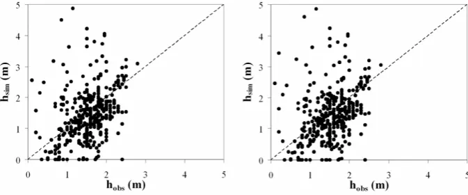
Figure 7. Dotty plots related to the calibrations with 390 data points and calibration strategies

C (left) and F (right).

37

Fig. 7. Dotty plots related to the calibrations with 390 data points and calibration strategies C (left) and F (right).

Figure 8. Dotty plots related to the calibrations with 343 data points and calibration strategies

C (left) and F (right).

38

Fig. 8. Dotty plots related to the calibrations with 343 data points and calibration strategies C (left) and F (right).

Figure 9. Dotty plots related to the calibrations with 143 data points and calibration strategies

C (left) and F (right).

Fig. 9. Dotty plots related to the calibrations with 143 data points and calibration strategies C (left) and F (right).

by roughness parameterization, this is rather a model error, i.e. the DEM. The most severe errors are removed when us-ing 343 data points, as illustrated in Fig. 8, where especially all severe underpredictions are removed thus causing the im-proved BIAS. Also, MAE and RMSE improve in the same rate as the BIAS. Using only 143 calibration points the BIAS is removed almost completely, as shown in Fig. 9. Corre-sponding to the reduced scatter also the MAE and RMSE drop significantly.

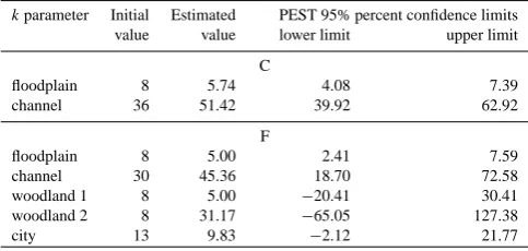
Comparing the actual estimated roughness values and the associated confidence intervals for the different number of data sets used in the calibrations given in Tables 6 and 7, it can be observed that the actual roughness estimates do not differ much between the different data sets, except for class woodland 2. However, it has to be noted that this area is lo-cated directly upstream of the cities railway station and track, which crosses the valley orthogonally and has the highest el-evation in the floodplain. Therefore it can be reasoned that

922 P. Fabio et al.: Towards automatic calibration of 2-D flood propagation models

Table 5. Goodness fit criteria of calibrated model results after removing points with low|CV|.

Number of Calibration No. points SQ (m2) BIAS (m) MAE (m) RMSE (m) parameters

Calibrations with 390 observed depths

2 C 390 264.9 0.083 0.594 0.824 5 F 390 263.4 0.089 0.589 0.822

Calibrations with 343 observed depths

2 C 343 189.4 0.019 0.530 0.743 5 F 343 187 0.018 0.522 0.738

Calibrations with 143 observed depths

2 C 143 7.2 0.003 0.177 0.224 5 F 143 5.2 0.005 0.058 0.202

Table 6. Calibration results as given by PEST considering 343 data

points.

kparameter Initial Estimated PEST 95% percent confidence limits

value value lower limit upper limit

C

floodplain 8 5.74 4.08 7.39

channel 36 51.42 39.92 62.92

F

floodplain 8 5.00 2.41 7.59

channel 30 45.36 18.70 72.58

woodland 1 8 5.00 −20.41 30.41

woodland 2 8 31.17 −65.05 127.38

city 13 9.83 −2.12 21.77

the influence of this particular area on the inundation process is largely overruled by the barrier imposed by the railways tracks directly downstream of it. This means in consequence that the simulation results are insensitive to the roughness parameterization in this land use class.

In contrast to the actual estimated roughness values the confidence intervals associated to the values differ consid-erably between the two calibrations with reduced data sets. Whereas with 343 remaining data points the confidence in-tervals hardly change compared to the original data set, they are significantly reduced using only 143 data points. Follow-ing the rational applied above, that the confidence intervals can serve as an indicator of the equifinality of the model pa-rameterisation, it can be reasoned that equifinality is reduced in this calibration approach. This, in turn, would also point into the direction of a match in model and data complexity.

5 Conclusions

In the present study an automatic calibration procedure has been applied to a 2-D hydraulic model utilising a

Table 7. Calibration results as given by PEST considering 143 data

points.

kparameter Initial Estimated PEST 95% percent confidence limits

value value lower limit upper limit

C

floodplain 8 5.52 4.79 6.25

channel 36 52.17 47.03 57.31

F

floodplain 8 5.00 3.93 6.07

channel 30 47.41 37.96 56.85

woodland 1 8 8.63 −6.60 23.85

woodland 2 8 5.00 −7.75 17.75

city 13 8.81 5.12 12.50

comprehensively data set of maximum inundation depths for a flood event occurred in August 2002 in Eilenburg, Ger-many. The optimiser used was the Parameter ESTimation tool PEST implementing a gradient based minimum search method of the objective function. The method proved to be effective in calibrating the model for different parameterisa-tion strategies. However, by applying different parameteri-sations and the confidence intervals computed for the esti-mated roughness values equifinality of model parameterisa-tions could be detected. In particular, with the proposed cal-ibration layout two model setups that perform equally well could be identified. Contrary to the usual case of complex models with large degrees of freedom in the parameter space, which are calibrated against just a few or bulk data, we could illustrate that the opposite situation may also cause equifi-nality: large degrees of freedom in the data in contrast to a comparatively simple model setup/parameterisation.

responsible alone or can we detect errors in data or model setup. To find answers to this question a method for the identification of possible erroneous data points was devel-oped based on the coefficient of variance between the dif-ferent calibration strategies for every calibration point. This method proved to be successful in improving the model cali-bration by removing data points with low coefficient of vari-ations from the calibration data set. Dotty plots of observed and simulated water depths confirmed the effectiveness of this approach. Moreover, the removal of the points could partly be explained and justified by DEM errors and reso-lution. In line with the findings that improving accuracy of DEM data could improve the reliability of flood inundation models (Werner et al., 2005b), that a model that gives a good overall fit to the available data may not give locally good re-sults (Pappenberger et al., 2007), and that the quality of the calibration data is essential for results, the proposed meth-ods helps in identifying erroneous calibration data points that otherwise obstruct proper model calibration. Also, the selec-tion of an appropriate model parameterisaselec-tion can be sup-ported by the presented method.

However, it has to be noted that above a certain number of removed points, i.e. a certain level of coefficient of variance, no unique or plausible explanation for the removal can be given. However, there are indications that by the removal of about half of the data points a match in model and data com-plexity is reached, thus enabling a significantly better model calibration and a reduction of equifinality.

While this study gives first insights in the possibilities of automatic calibration of 2-D hydraulic models and the detection of equifinality and erroneous calibration data points, a number of questions remain open: Is the gradient based method efficient in finding the global maximum? How to implement multi-objective optimisations considering e.g. maps of flood inundation extends and time series of discharge and stage at various points in the simulation domain? How to determine the optimal match between data and model complexity? How to consider the uncertainty in calibration data in the automatic calibration? These questions will be the challenges in research for the scientific community in the coming years.

Edited by: J. Freer

References

Apel, H., Aronica, G. T., Kreibich, H., and Thieken, A. H.: Flood risk analyses – how detailed do we need to be?, Nat. Hazards, 49, 79–98, 2009.

Aronica, G., Bates, P. D. and Horritt, M. S.: Assessing the uncer-tainty in distributed model predictions using observed binary pat-tern information within GLUE, Hydrol. Process., 16(10), 2001– 2016, 2002.

Aronica, G., Hankin, B., and Beven, K.: Uncertainty and equifi-nality in calibrating distributed roughness coefficients in a flood propagation model with limited data, Adv. Water Resour., 22(4), 349–365, 1998b.

Aronica, G. T., Tucciarelli, T., and Nasello, C.: 2-D multi-level model for flood Wave propagation in flood-affected areas, J. Wa-ter Res. Pl.-ASCE, 124(4), 210–217, 1998a.

Bales, J. D. and Wagner, C. R.: Sources of uncertainty in flood inundation maps, J. Flood Risk Manag., 2(2), 139–147, 2009. Bates, P. D.: Remote sensing and flood inundation modeling,

Hy-drol. Process., 18(13), 2593–2597, 2004.

Bates, B.C., and De Roo, A.P.J.: A simple raster-based model for flood inundation simulation. Journal of Hydrology, 236(1-2), 54-77, 2000.

Bates, B. C. and Townley, L. R.: Nonlinear, discrete flood event models, 1. Bayesian estimation of parameters, J. Hydrol., 99, 61– 76, 1988.

Beven, K. J.: Prophecy, reality and uncertainty in distributed hydro-logical modelling, Adv. Water Resour., 16(1), 41–51, 1993. Beven, K. J.: Equifinality and uncertainty in geomorphological

modelling, in: The Scientific Nature of Geomorphology, edited by: Roads, B. L. and Thorn, C. E., Wiley, Chichester, 289–313, 1996.

Beven, K. J.: A manifesto for the equifinality thesis, J. Hydrol., 320, 18–36, 2006.

Beven, K. J. and Binley, A. M.: The future of distributed models: model calibration and uncertainty prediction, Hydrol. Process., 6(3), 279–298, 1992.

Beven, K. J. and Freer, J.: Equifinality, data assimilation, and uncer-tainty estimation in mechanistic modelling of complex environ-mental systems using the GLUE methodology, J. Hydrol., 249, 11–29, 2001.

Chow, V.: Open Channel Hydraulics, McGraw-Hill, New York, 1959.

Doherty, J.: PEST: Model Independent Parameter Estimation. Fifth edition of user manual, Watermark Numerical Computing, Bris-bane, Australia, 2004.

Doherty, J.: Addendum to the PEST Manual, Watermark Numerical Computing, Brisbane, Australia, 2008.

Duan, Q., Gupta, V. K., and Sorooshian, S.: Shuffled Complex Evo-lution Approach for Effective and Efficient Global Minimization, J. Optimiz. Theory Appl., 76(3), 501–521, 1993.

Duan, Q., Sorooshian, S., and Gupta, V. K.: Effective and Effi-cient Global Optimization jbr Conceptual Rainfall-Runoff Mod-els, Water Resour. Res., 28(4), 1015–1031, 1992.

Gupta, H. V., Sorooshian, S., and Yapo, P. O.: Toward improved cal-ibration of hydrologic models: Multiple and noncommensurable measures of information, Water Resour. Res., 34(4), 751–763, 1998.

Horritt, M. S: a methodology for the validation of uncertain flood inundation models, J. Hydrol., 326(1–4), 153–165, 2006. Horritt, M. S., Di Baldassare, G., Bates, P. D. and Brath, A.:

Com-paring the performance of a 2-D finite element and a 2-D fintite volume model of floodplain inundation using airborne SAR im-agery, Hydrol. Process., 21, 2745–2759, 2007.

924 P. Fabio et al.: Towards automatic calibration of 2-D flood propagation models

Hunter, N. M., Bates, P. D., Horritt, M. S., De Roo, P. J., and Werner, M. G. F.: Utility of different data types for calibrat-ing flood inundation models within a GLUE framework, Hydrol. Earth Syst. Sc., 9(4), 412–430, 2005.

Hunter, N. M., Bates, P. D., Horritt, M. S., and Wilson, M. D.: Sim-ple spatially-distributed models for predicting flood inundation: A review, Geomorphology, 90, 208–225, 2007.

Levenberg, K.: A method for the solution of certain non-linear problems in least squares, Q. Appl. Math., 2, 164–168, 1944. Marks, K. and Bates, P. D.: Integration of high-resolution

topo-graphic data with floodplain flow models, Hydrol. Process., 14, 2109–2122, 2000.

Marquardt, D.: An algorithm for least-squares estimation of non-linear parameters, J. Soc. Indust. Appl. Math., 11(2), 431–441, 1963.

Mignot, E., Paquier, A., and Haider, S.: Modelling floods in a dense urban area using 2D shallow water equations, J. Hydrol., 327(1– 2), 186–199, 2006.

Neal, J. C., Bates, P. D., Fewtrell, T. J., Hunter, N. M., Wilson, M. D., and Horritt, M. S.: Distributed whole city water level mea-surements from the Carlisle 2005 urban flood event and com-parison with hydraulic model simulations, J. Hydrol., 368(1–4), 42–55, 2009.

Pappenberger, F., Beven, K., Frodsham, K., Romanowicz, R., and Matgen, P.: Grasping the unavoidable subjectivity in calibration of flood inundation models: A vulnerability weighted approach, J. Hydrol., 333, 275–287, 2007.

Pappenberger, F., Beven, K., Horritt, M., and Blazkova, S.: Un-certainty in the calibration of effective roughness parameters in HEC-RAS using inundation and downstream level observations, J. Hydrol., 302, 46–69, 2005.

Romanowicz, R. and Beven, K.: Estimation of flood inundation probabilities as conditioned on event inundation maps, Water Re-sour. Res., 39(3), W1073, doi:10.1029/2001WR001056, 2003. Schumann, G., Matgen, P., Hoffmann, L., Hostache, R.,

Pappen-berger, F., and Pfister, L.: Deriving distributed roughness values from satellite radar data for flood inundation modelling, J. Hy-drol., 344(10–2), 96–111, 2007.

Schwarz, J., Maiwald, H., and Gerstberger, A.: Quantifizierung der Sch¨aden infolge Hochwassereinwirkung: Fallstudie Eilenburg, Bautechnik, 82(12), 845–856, 2005.

Sorooshian, S., Duan, Q., and Gupta, V. K.: Calibration of rainfall-runoff models: application of global optimization to the Sacra-mento soil moisture accounting model, Water Resour. Res., 29(4), 1185–1194, 1993.

Werner, M. G. F., Blazkova, S., and Petr, J.: Spatially distributed observations in constraining inundation modelling uncertainties, Hydrol. Process., 19, 3081–3096, 2005a.

Werner, M. G. F., Hunter, N. M., and Bates, P. D.: Identifiability of distributed floodplain roughness values in flood extent estima-tion, J. Hydrol., 314, 139–157, 2005b.