www.hydrol-earth-syst-sci.net/20/3477/2016/ doi:10.5194/hess-20-3477-2016
© Author(s) 2016. CC Attribution 3.0 License.
Quantifying shallow subsurface water and heat dynamics
using coupled hydrological-thermal-geophysical inversion
Anh Phuong Tran, Baptiste Dafflon, Susan S. Hubbard, Michael B. Kowalsky, Philip Long, Tetsu K. Tokunaga, and Kenneth H. Williams
Climate & Ecosystems Division, Earth and Environmental Sciences Area, Lawrence National Berkeley Lab, Berkeley, CA 94720, USA
Correspondence to:Anh Phuong Tran ([email protected])
Received: 20 April 2016 – Published in Hydrol. Earth Syst. Sci. Discuss.: 25 April 2016 Revised: 26 July 2016 – Accepted: 17 August 2016 – Published: 31 August 2016
Abstract. Improving our ability to estimate the parameters that control water and heat fluxes in the shallow subsur-face is particularly important due to their strong control on recharge, evaporation and biogeochemical processes. The objectives of this study are to develop and test a new inver-sion scheme to simultaneously estimate subsurface hydrolog-ical, thermal and petrophysical parameters using hydrologi-cal, thermal and electrical resistivity tomography (ERT) data. The inversion scheme – which is based on a nonisothermal, multiphase hydrological model – provides the desired sub-surface property estimates in high spatiotemporal resolution. A particularly novel aspect of the inversion scheme is the explicit incorporation of the dependence of the subsurface electrical resistivity on both moisture and temperature. The scheme was applied to synthetic case studies, as well as to real datasets that were autonomously collected at a biogeo-chemical field study site in Rifle, Colorado. At the Rifle site, the coupled hydrological-thermal-geophysical inversion ap-proach well predicted the matric potential, temperature and apparent resistivity with the Nash–Sutcliffe efficiency crite-rion greater than 0.92. Synthetic studies found that neglecting the subsurface temperature variability, and its effect on the electrical resistivity in the hydrogeophysical inversion, may lead to an incorrect estimation of the hydrological parame-ters. The approach is expected to be especially useful for the increasing number of studies that are taking advantage of au-tonomously collected ERT and soil measurements to explore complex terrestrial system dynamics.
1 Introduction
Shallow subsurface moisture and temperature are two pri-mary variables that play key roles in hydrological and bio-geochemical processes in terrestrial environments. For exam-ple, watershed moisture content and temperature are the main factors that control the partitioning of precipitation into evap-otranspiration, infiltration and runoff (Merz and Bardossy, 1998; Brocca et al., 2010). For ecosystems, moisture content and temperature conditions are closely linked to form, func-tioning and organization of vegetation, which in turn influ-ence ecological diversity (Rodriguez-Iturbe, 2000). Subsur-face moisture and temperature largely influence microbial ac-tivity in the subsurface, including respiration of greenhouse gases (Boone et al., 1998; Luo et al., 2013). However, moni-toring the variability of subsurface moisture and temperature over spatiotemporal scales that are relevant to the local pro-cesses yet informative for predicting watershed or ecosys-tem functioning is challenging. Conventional point-sensing approaches can provide subsurface moisture and tempera-ture. However, due to labor and costs involved in installing point-sensing systems and the invasive nature of the sensors, the spatial support scale of point-sensing systems is typically quite small compared to the scale of systems of interest.
and electrical resistance tomography (ERT). For example, Hubbard et al. (2001) applied a Bayesian algorithm to inte-grate surface and cross-hole GPR, seismic cross-hole tomog-raphy, cone penetrometer, borehole electromagnetic flowme-ter and pumping tests to estimate the spatial distribution of subsurface hydraulic conductivity. Binley et al. (2002) esti-mated shallow subsurface hydraulic conductivity using both cross-well ERT and GPR. Doetsch et al. (2010) showed that merging seismic, GPR and ERT data could significantly im-prove the accuracy of aquifer zonation and associated zonal parameter estimation. Dafflon and Barrash (2012) used a stochastic approach to estimate the distribution of porosity from well data and GPR data. Tran et al. (2015) combined surface GPR and frequency domain reflectometry data to bet-ter quantify the spatiotemporal dynamics of moisture along a hillslope.
Coupled hydrogeophysical inversion approaches have also been developed to estimate soil hydrological parameters, which assimilate all geophysical and other key datasets into a model that consider physical hydrodynamics (i.e., Darcy’s law) and electromagnetic laws (i.e., Maxwell’s equations). Because coupled inversion approaches permit direct use of geophysical data for inversion, they avoid the errors typ-ically associated with geophysical inversion process (e.g., Binley et al., 2002; Singha and Gorelick, 2005) and associ-ated resolution issues (Day-Lewis and Lane, 2004). Kowal-sky et al. (2005) and Lambot et al. (2009) developed coupled inversion schemes and used time-lapse GPR data to estimate hydraulic conductivity and matric potential functions. John-son et al. (2009) jointly inverted time-lapse hydrogeologic and ERT data without a priori assumptions about petrophys-ical parameters. Using ERT data, Huisman et al. (2010) de-veloped a coupled Bayesian hydrogeophysical inversion ap-proach to determine the hydraulic properties and their un-certainties of flood-protection dikes. Kowalsky et al. (2011) employed time-lapse ERT, groundwater level and nitrate concentration data to estimate hydrogeochemical parameters and behavior of a contaminated subsurface system. Tran et al. (2014) developed a data assimilation scheme that is based on the maximum-likelihood ensemble filter technique to se-quentially estimate the vertical soil moisture profile and pa-rameters of water retention and hydraulic conductivity func-tions using full-wave GPR data.
To date, ERT is the geophysical technique that is most commonly collected in an autonomous manner for near-surface applications. ERT provides information about the distribution of subsurface electrical resistance; a review of ERT theory and inversion procedures is given by Binley and Kemna (2005). Due to the typically high sensitivity of electri-cal resistivity to pore fluid conductivity and saturation, ERT has been used widely for monitoring the vadose zone soil moisture and other terrestrial system processes (e.g., Binley et al., 2002; Kemna et al., 2002; McClymont et al., 2013; Hubbard et al., 2013). However, because the electrical resis-tivity is also sensitive to other subsurface properties (such
as porosity, tortuosity, pore-grain electrochemistry, mineral-ogy and temperature), other measurements must be used with ERT to avoid large estimation errors (Binley et al., 2002). For example, dependence of subsurface electrical resistiv-ity on temperature is well known but often not adequately accounted for in hydrogeophysical approaches. The subsur-face temperature directly influences the subsursubsur-face electri-cal resistivity. It also controls the phase change of subsur-face moisture, which ultimately affects the subsursubsur-face resis-tivity. In some cases, subsurface temperature variations affect subsurface resistivity more than moisture variations (Rein et al., 2004; Musgrave and Binley, 2011). The conventional ap-proach for correcting for temperature effects on ERT data in-cludes inverting data and then performing correction on the obtained resistivity/conductivity images (Hayley et al., 2007; Ma et al., 2014). This approach is not suitable for the coupled hydrogeophysical inversion, because the objective of the hy-drogeophysical inversion is to estimate hydrological param-eters (not electrical resistivity/conductivity image). Hayley et al. (2010) proposed a temperature-compensation approach that removes the temperature effect on the data before inver-sion, which appeared to better resolve the temperature de-pendence of the electrical resistivity. This approach can be used for the hydrogeophysical inversion. However, this ap-proach first requires the inversion of electrical resistance data to obtain the correction factors. Secondly, the correction usu-ally relies on temperature measurements at several specific points in time, which may not suffice due to high variabil-ity of moisture and temperature in space and time. To date, few studies have incorporated and evaluated the effect of the relationship between subsurface resistivity and temperature within a coupled hydrogeophysical inversion scheme.
We organize this article as follows. Section 2 describes the development of the hydrological-thermal-geophysical inver-sion scheme. The application of the inverinver-sion scheme to the Rifle site study is described in Sect. 3. Section 4 compares two synthetic cases that perform geophysical inversion, with and without considering the subsurface temperature’s influ-ence. Section 5 offers a summary and concluding remarks.
2 Methodology
2.1 Hydrological forward model
In this study, we simulated the nonisothermal two-phase (gas and liquid), three-component (air, water and heat) flow in the vadose zone using the integral finite-difference simulator TOUGH2 (Transport of Unsaturated Groundwater and Heat; Pruess et al., 1999). TOUGH2 solves the mass and energy balance equations for each component over an arbitrary vol-umeV, confined by a closed surface0of the flow computa-tional domain, which is written in the integral form as below: Z
V
Mkdv=
Z
0
Fknd0+
Z
V
qkndv, (1)
in whichMis the mass or energy accumulation term for com-ponentk;F represents the mass or heat flux;q denotes the sink or source terms; andnis the normal vector on the sur-face elementd0. The mass accumulation term is defined as
Mk=φX
β
SβρβXkβ, (2)
whereφis the porosity;Sβ andρβ are, respectively, the
sat-uration and density of phaseβ; andXkβ is the mass fraction of phaseβ in componentk. For simulating the nonisother-mal problem, the heat accumulation component (Mh) is also accounted for:
Mh=(1−φ)ρRCRT +φ
X
β
Sβρβuβ, (3)
where ρR and CR are, respectively, the grain density and
specific heat capacity of the soil/sediment particle materials;
T is the temperature; anduβis the specific internal energy in
phaseβ.
The mass flux termFkof componentkis the sum of all of its phase fluxes:
Fk=X
β
fβXβk, (4)
with
fβ = −K
krβ
µβ
ρβ ∇Pβ−ρβg−φSβkdβk∇Xkβ. (5)
The first term in Eq. (5) represents the advection. The sec-ond one describes the molecular diffusion. K is the abso-lute permeability;krβis the relative permeability of phaseβ;
Pβ=Pref+Pcdenotes the pressure, in whichPrefandPcare
the reference gas pressure and matric potential; dβk and
µβ are the molecular diffusion coefficient and viscosity of
phaseβ, respectively; andgis the gravitational acceleration. For gas phase (air and vapor), the diffusion coefficient is a function of pressure and temperature as
dgk=dgk(P0T0)
P0
P
T +273.15 273.15
1.8
, (6)
wheredgk(P0T0) is the gas diffusion coefficient at the
stan-dard condition P0=1 atm, and T0=0◦C. The
relation-ship between the matric potential, the relative permeability and the water saturation is formulated by Mulem and van Genuchten (van Genuchten, 1980) as
Pc= −
1
α
Se−1/m−1
1−m
, (7)
krl=
p
Se
h
1−1−Se1/m
mi2
. (8)
The relative permeability of the gas phase is described by Corey (1954) as
krg=
(
(1− ˆS)21− ˆS2 ifSgr>0
1−krl ifSgr=0
, (9)
whereSeandSˆare defined as
Se=
Sl−Slr
Sls−Slr
, (10)
ˆ
S= Sl−Slr
1−Slr−Sgr
, (11)
in whichSlsrepresents the saturated liquid saturation;Slrand
Sgr are the residual liquid and gas saturation, respectively;
mrepresents the pore size distribution of the soil/sediment; andαis inversely proportional to the air-entry pressure. Heat fluxes consist of conductive and convective components:
Fh= −λ∇T +X
β
hβfβ, (12)
whereλdemotes the thermal conductivity andhβis the
spe-cific enthalpy in phaseβ. It is worth noting that the evap-oration was accounted for by the diffusion term in Eq. (5). However, the current version of TOUGH2 does not consider the root water uptake and transpiration from vegetation. 2.2 ERT forward model
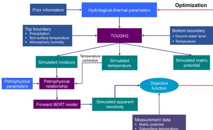
Figure 1.Flowchart showing the steps involved in the coupled hydrological-thermal-geophysical inversion scheme. The objective function is represented by Eq. (15). Estimated parameters consist of hydrological-thermal and petrophysical parameters (blue rectangles). The navy blue rectangles denote the model inputs, including prior information about estimated parameters, and the top and bottom boundary conditions. The purple rectangles denote the forward TOUGH2, geophysical and petrophysical models. The teal and indigo rectangles, respectively, denote the simulation and measurement. Data for inversion in this study include matric potential, subsurface temperature and apparent resistivity.
solves Poisson’s equation using the finite-element method in a three-dimensional, arbitrary topography. By incorporating unstructured, tetrahedral meshes, the model enables efficient refinement of the local mesh, and flexibly describes any ge-ometry of the computational domain. The use of quadratic shape functions also helps to improve the accuracy of the simulation.
2.3 Petrophysical model
The bulk electrical conductivity (σb) includes contributions
from the electrical conductivity of pore water and the surface conduction at the pore and water–mineral interface (Revil et al., 2012). We employed the model proposed by Linde et al. (2006), which was extended from Archie’s model (Archie, 1942), and is expressed below as
σb=φd
h
Snlσw+
φ−d−1σs
i
, (13)
whered is the cementation index;nis the saturation index; andσwandσsare, respectively, the electrical conductivity of
water and soil/sediment surface conduction. Equation (13) indicates that the cementation and saturation indexes closely correlate. Hence, to reduce the number of unknown param-eters and ameliorate nonuniqueness, we set the cementation index atd=1.3, which is commonly used for unconsolidated sand (Archie, 1942). The electrical conductivity of pore wa-ter, which does not vary significantly over time at the Rifle site, was taken from the measurements at the nearby well and is equal to 0.244 S m−1. In the case that the spatiotemporal
variation of solute concentration and resulting electrical con-ductivity in pore water are significant, its dynamics should be simulated by considering it as a component in TOUGH2. A formula that links the solute concentration with the water electrical conductivity also needs to be developed.
The relationship between temperature and electrical con-ductivity can be formulated using linear (Sen and Goode, 1992) or exponential (Llera et al., 1990) equations. In this study, we chose the linear form:
σbT =σb[1+c(T−25)], (14)
in whichT is the temperature;σbT is the electrical resistivity at temperatureT ◦C; andcis the temperature-compensation factor, corresponding to 25◦C. The valuec=0.0183◦C−1as suggested by Hayley et al. (2007) was used for our study. 2.4 Coupled hydrological-thermal-geophysical
inversion scheme
to the BERT mesh; (5) execute the forward BERT model to simulate the electrical resistance from the resistivity image; (6) convert the electrical resistance to the apparent resistiv-ity using geometric factors; and (7) minimize the misfit be-tween simulation and measurement of the apparent resistivity and other hydrological-thermal (matric potential and temper-ature) data to estimate hydrological-thermal and petrophys-ical parameters. The misfit is formulated by the objective function as below:
8(p)=eTC−1e, (15)
wheree=z∗−z(θ,p)is the residual vector quantifying the difference between the modeled (z) and measured (z∗) data; pandθare, respectively, the vectors representing the model parameters and input data; andCdenotes the covariance ma-trix of measurements errors. We assumed that there is no correlation between measurement errors, and therefore the covariance matrixCbecomes a diagonal matrix in which the main diagonal elements are the variances of measurement er-rors. It is worth noting that the vectors z,z∗ and matrixC
can contain multiple data types. The difference in units as-sociated with the different data types was removed by the covariance matrix of the measurement errors. For parame-ter estimation, we used the Levenberg–Marquardt algorithm (Marquardt, 1963) for nonlinear optimization.
The agreement between measured and modeled data was evaluated using the Nash–Sutcliffe efficiency coefficient:
NSE=1− e
Te
n0σ02
, (16)
where σ02 is the variance of the measured data and n0 is
the number of measurements. The Nash–Sutcliffe coefficient ranges from−∞to 1. The modeled and measured data per-fectly agree if this coefficient equals 1. A coefficient of 0 implies that the model prediction is as accurate as the mean of the measured data; a value less than 0 indicates that the model prediction is worse than the measured mean.
The uncertainties of estimated parameters are character-ized by their standard deviation values, which are the square root of the diagonal elements of the covariance matrix of the estimated parameters:
σpi=
q
Cppii, (17)
wherei=1, . . . ,np. The covariance matrix of the estimated
parameters is computed as Cpp=s2
JTC−1J
−1
, (18)
whereJis the Jacobian matrix ands2 is an estimate of the error variance:
s2=e
TC−1e
n0−np
. (19)
Good initial guesses can help to avoid local minima with unrealistic solutions. As such, we implement the following practical procedure to progressively approach an optimal so-lution:
1. Invert the matric potential data to obtain the subsurface hydrological parameters. In this step, we consider only the one-dimensional isothermal hydrological model. 2. Use the subsurface temperature data to estimate the
thermal parameters of the one-dimensional nonisother-mal hydrological model. The subsurface hydrological parameters obtained in step 1 are fixed and are used to simulate the hydrological processes.
3. Jointly invert the matric potential, temperature and apparent-resistivity data to obtain the subsurface hydrological-thermal and petrophysical parameters. The hydrological-thermal parameters from steps 1 and 2 are used as the initial guesses for this step. In this step, the inversion is performed for the two-dimensional non-isothermal hydrological model.
In each step, global sensitivity analysis is performed to eval-uate the sensitivity of the calibration data with respect to the model parameters. The insensitive parameters (the sensitivity coefficient is approximately equal to 0) are not considered in inversion. We apply the global sensitivity analysis method re-ferred to as one-step-at-a-time (OAT) Morris method, which is available in iTOUGH2 (Wainwright et al., 2013). This method is briefly described as follows: the parameter space ofnpparameters is normalized to thenp-dimensional domain
([0, 1]np). Each dimension of this normalized domain is dis-cretized intons−1 equal segments, generatingnsgrid points
that take values in the set{0, 1/(ns−1), 2/(ns−1), . . . 1}.
The element effect (EEj(pi)) of parameterpi at an arbitrary
grid point with respect to model outputzis defined as
EEj(pi)=
1
F
zp1j, . . ., pij+1, . . ., p j np
−zp1j, . . ., pij, . . ., p j np
1 ,, (20)
in whichpj≤1−1, with1= ns
2(ns−1), andF is the scaling factor for comparing the element effects of different mea-surementsz. The element effect quantifies the variation of the model output with respect to variation of parameterpiat
a given point in the parameter space. To evaluate the param-eter sensitivity, we need to calculate the element effects of all parameters at all grid points, which requires a large com-puting resource. To overcome this constraint, Morris (1991) generated several random sample paths and computed the el-ement effects of each parameter along these paths. The sen-sitivity coefficient|EE(pi)| = 1
ns j=ns
P
j=1
|EEj (pi)| determines
the sensitivity of parameterpi. A parameter with a higher
3 Field study
3.1 Study site and datasets
The newly developed approach was tested at a floodplain adjoining the Colorado River, near Rifle, Colorado (USA) (Fig. 2). The perched aquifer at the site overlies low-permeability mud and siltstones of the Eocene Wasatch For-mation. Above the Wasatch Formation is a Quaternary allu-vial layer consisting of sandy, gravelly unconsolidated sedi-ments. The uppermost layer is a silty clay fill with a thickness of around 1.5–2 m, which replaced contaminated soils and sediments removed from the site following uranium recla-mation activities. Groundwater elevations fluctuate season-ally with snowmelt infiltration and Colorado River stage, and vary from around 3.5 to 2.4 m below ground surface.
The Berkeley Lab and others in the scientific community have performed many studies at the Rifle site to explore com-plex subsurface hydro-biogeochemical behavior and to test the development of new characterization and modeling ap-proaches. For example, Li et al. (2010) used reactive trans-port modeling to investigate the influence of physical and geochemical heterogeneities on the spatiotemporal distribu-tion of mineral precipitates and biomass that formed during a biostimulation experiment. Yabusaki et al. (2011) developed a three-dimensional hydro-biogeochemical reactive transport model of Rifle to improve understanding of the uranium variability, hydrological conditions and soil properties under the pulsed acetate amendment. Chen et al. (2013) developed a data-driven biogeophysical approach to quantify redox-driven biogeochemical transformations using geochemical measurements and induced polarization data. Wainwright et al. (2015) used induced polarization data and stochastic methods to estimate the spatial distribution of naturally re-duced zones in the subsurface, which served as biogeochem-ical hot spots; the geophysbiogeochem-ical information was used to con-strain simulations of biogeochemical cycles across the Rifle floodplain. Arora et al. (2016) used reactive transport mod-eling approaches to explore seasonal variations in biogeo-chemical fluxes occurring from bedrock to canopy as well as laterally to the Colorado River. They found that CO2
con-centration in the unsaturated zone could not be accurately re-produced without incorporating temperature gradients in the simulations and that incorporating temperature fluctuations resulted in an increase in the annual groundwater carbon fluxes to the river by 170 %. They concluded that spatial mi-crobial and redox zonation as well as temporal fluctuations of temperature and water table depth contributed significantly to subsurface carbon fluxes in the Rifle floodplain, and they identified the need to represent temperature and moisture dy-namics for accurate model simulations.
[image:6.612.312.538.67.209.2]In this study, we tested our new approach using data collected along a Rifle, CO ERT transect, which includes 112 electrodes with a distance between any two adjacent electrodes of 1 m (Fig. 2). The ERT data were autonomously
Figure 2.Plan view of the Rifle floodplain of the Colorado River, Colorado, and the location of the TT02 and TT03 wells and ERT line.
collected every day from April through June 2013 using the Wenner electrode array. These data were used for two pur-poses: (1) determining subsurface stratigraphy to support construction of the hydrological model and (2) estimating hydrological-thermal and petrophysical parameters through the coupled inversion approach.
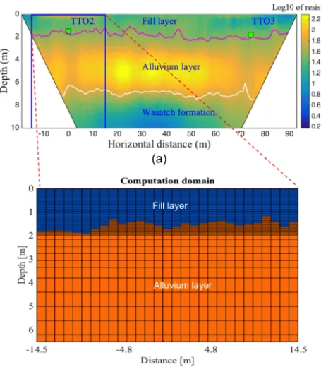
For characterizing subsurface stratigraphy and specifying the depths of the fill, alluvium and Wasatch layers, we used the BERT inversion package (Günther et al., 2006) to in-vert the ERT data that were collected on 20 May 2013. The electrical resistivity image obtained by inversion is shown in Fig. 3a. As expected, the clay-rich fill and Wasatch layers ex-hibit less resistivity than the alluvium layer. To specify the lo-cations of the fill–alluvium and alluvium–Wasatch interfaces from ERT geophysical inversion, we used the depths of these interfaces observed at the TTO2 and TTO3 wells as the refer-ences to determine resistivity thresholds. Accordingly, a grid cell with a resistivity greater than 1.52log10(m) and above 1.5 m depth belongs to the alluvium layer. The cells whose resistivity values are smaller than 1.83log10(m) and below 5 m are assigned to the Wasatch layer. The remaining cells are in the fill layers. The magenta and white lines in Fig. 3 represent the fill–alluvium and alluvium–Wasatch interfaces, respectively.
We developed a computational domain that is a rectangle centered at the TT02 well, with a width of 30 m, as shown in Fig. 3b. Previous work at this site has suggested that the spatial variability over the extent of the simulation transect is not likely to be significant (Li et al., 2010). Consequently, we assumed the computational domain includes two homo-geneous layers: namely, fill and alluvium. The porosity is 0.4 for the fill and 0.2 for the alluvium layer (Tetsu K. Toku-naga, personal communication, 2015). The top boundary of the domain is the atmospheric layer, and the bottom is the impermeable Wasatch layer. We set the depth of the bot-tom boundary at the average depth of the Wasatch layer,
Figure 3. (a)The 2-D image of the soil electrical resistivity ob-tained by inverting ERT data collected on 20 May 2013. The magenta and white lines delineate the inferred fill–alluvium and alluvium–Wasatch boundaries, respectively. Green square markers denote the fill–alluvium boundary determined from the well logs of TT02 and TT03 and adjacent wells, as recorded in the field dur-ing drilldur-ing. The blue rectangular box indicates the hydrological-thermal computational domain.(b)Computational domain for the hydrological-thermal inversion with associated grid mesh. Blue and orange regions represent the fill and alluvium layers, respectively. The domain is situated below an atmospheric layer (top boundary) and above the relatively impermeable Wasatch (bottom boundary).
columns, each with a size of 1 m in the horizontal direction. In the vertical direction, the cell size is 0.05 m for the upper-most 2 mm, 0.3 m for the next 1.5 m and 0.6 m for the last 3 m, for a total of 1560 cells. The BERT computational mesh was automatically generated in BERT. We set the maximum cell size which controls the mesh refinement at a small value (0.2 m) to capture the local variation of the soil electrical re-sistivity. Other parameters that determine the BERT compu-tational mesh were kept as their default values. For more in-formation about BERT mesh generation, we refer to Rücker et al. (2006). The apparent resistivity was mapped from the hydrological to the BERT mesh using the nearest-distance method; i.e., a cell in the BERT mesh will get the resistivity value of its nearest cell in the hydrological mesh. The electri-cal resistivity of the Wasatch layer was set at its average value obtained from geophysical inversion (ρbWasatch=45m).
We performed the hydrological-thermal simulation dur-ing the snow-free period from 4 May 2013 to 25 Novem-ber 2013 (194 days). All meteorological data (atmospheric
pressure, temperature, humidity and rainfall) were measured at a nearby meteorological station. The surface boundary conditions include land surface temperature, atmospheric pressure, air mass fraction and rainfall. The land surface temperature was adjusted from the atmospheric tempera-ture, based on a regression approach proposed by Zheng et al. (1993), while the air mass fraction was calculated from the atmospheric pressure and relative humidity data. The bot-tom boundary condition of pressure was calculated from the groundwater table data, and the bottom temperature was ap-proximated from the land surface temperature. The initial conditions were derived from the measured data at the be-ginning of the simulation period. For more detailed informa-tion about initial and boundary condiinforma-tions, we refer to Tran et al. (2016).
Data for inversion included time-lapse matric potential, temperature and apparent-resistivity measurements. Assum-ing that the lateral variation in subsurface temperature be-tween TTO2 and TTO3 wells (see the TT03 location in Fig. 2) was insignificant, we used temperature data at the TTO3 well for inversion. Temperature was measured every 5 min at six depths below the surface:z=0.75, 1, 1.5, 2.5, 4.6 and 6 m. The 5 min data were averaged to obtain daily data. Using tensiometers, the matric potential was occasion-ally measured at the TTO2 well at depthsz=0.5, 1, 1.5, 2, 2.5 and 3 m. As for the ERT data, we chose six datasets that cover the most important variations of subsurface moisture and temperature during the measurement period. For each dataset, we selected 246 values obtained from 54 electrodes in and around the computational domain for inversion. The measurement errors were assumed to follow a standard Gaus-sian distribution. The standard deviation of the errors for the resistivity and matric potential data are 5 % of the measure-ment values. For the temperature data, because the instru-ment errors of the thermistors are from 0.1 to 0.4◦C, we as-sumed that the standard deviation of the errors for this type of measurement is 0.4◦C.
3.2 Results and discussion
All of the hydrological-thermal and petrophysical parame-ters that were considered in this study are presented in Ta-ble 1. The first and second columns present the parameter names and ranges, respectively. From the third to the last col-umn, we present the estimated parameters obtained from dif-ferent inversion cases, namely hydrological inversion (HI), thermal inversion (TI), and coupled hydrological-thermal-geophysical inversion (HTGI).
3.2.1 Sensitivity analysis
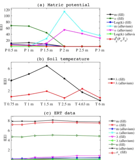
[image:7.612.52.280.66.326.2]sen-Figure 4.The sensitivity coefficients|EE|of matric potential, sub-surface temperature and apparent-resistivity data with respect to dif-ferent hydrological, thermal and petrophysical parameters. A pa-rameter with a higher|EE|is more likely to be determined.(a)The sensitivity coefficient|EE|of the matric potential at depths of 0.5, 1, 1.5, 2, 2.5 and 3 m, with respect to the hydrological parameters of the fill and alluvium layers, and the gas diffusion coefficient stan-dard conditions.(b)The|EE|of the temperature at depths of 0.75, 1, 1.5, 2.5, 4.63 and 6 m, with respect to the thermal conductivity of fill and alluvium layers.(c)The temporal variations of the|EE|of the resistivity data with respect to the soil hydrological-thermal and petrophysical parameters of both fill and alluvium layers.
sitive to the parameters of van Genuchten’s retention curve than to the absolute permeability. At the fill layer, the influ-ence of parameterαon the matric potential is significantly higher than the other parameters. The second-most-sensitive parameter ism. At the alluvium layer,αandmare also the two most sensitive parameters. The sensitivity coefficient of the absolute permeability of the fill layer (|EE|matric potential
Kfill )
is relatively small, and that of the alluvium permeability is nearly equal to 0. This can be explained by the lack of infil-tration during the simulation period. As a result, there is little information for estimating the absolute permeability, which controls the moisture dynamics. The retention curve param-eters determine the shape of the matric potential profile, and therefore the matric potential is more sensitive to them. Fig-ure 4a also shows that the hydrological parameters of a given layer are mostly sensitive to the matric potential measure-ments at that layer. For example, the|EE|matric potentialα
fill ofαof
the fill layer on the matric potential is around 45–68 for the fill layer and 0 for the alluvium layer (z >1.5 m). By con-trast, the|EE|matric potentialα
fill ofαof the alluvium layer on the matric potential is 35–114 for the alluvium layer and 0 for the fill layer. This implies that there was little moisture exchange between the two layers during the simulation period. Sensitivity of temperature with thermal parameters The sensitivity of the subsurface temperature data with re-spect to the thermal conductivity of the fill and alluvium lay-ers at depths from 0.75 to 6 m is depicted in Fig. 4b. The figure indicates that the sensitivity coefficient|EE|temperature
λfill of the thermal conductivity of the fill layer on temperature reaches its maximum atz=1.5 m (|EE|temperature
λfill =6.5) and its minimum atz=6 m (|EE|temperature
λfill =0.2). This implies that the temperature data at 1.5 m depth contain the most valuable information for estimating the thermal conductiv-ity of the fill layer. The temperature data at depthz=4.6 m are the most sensitive to the thermal conductivity of the al-luvium layer|EE|temperature
λalluvium =2.3, while the temperature data at depths 0.75, 2.5 and 6 m are the least sensitive, with the |EE|temperature
λalluvium roughly equal to 0.7. The figure also indicates that the subsurface temperature data at depths 0.75, 1, 1.5 and 2.5 m are much more sensitive to the thermal conductivity of the fill than to that of the alluvium layer. By contrast, be-low 2.5 m, the sensitivity of the temperature data to the ther-mal conductivity of the fill layer is slightly higher than to that of the fill layer. This is because temperature at shallower depths is more dynamic in both time and space than at deeper depths. As a result, there is more information for estimating the thermal conductivity of the shallower fill layer.
Sensitivity of apparent resistivity with
hydrological-thermal and petrophysical parameters Based on the above sensitivity analysis with the matric po-tential and temperature data, we selected the six most sensi-tive hydrological-thermal parameters (α,mandλ, for both fill and alluvium layers) for sensitivity analysis with the apparent-resistivity data. We also considered three petro-physical parameters, includingn(fill, alluvium) andσs( fill)
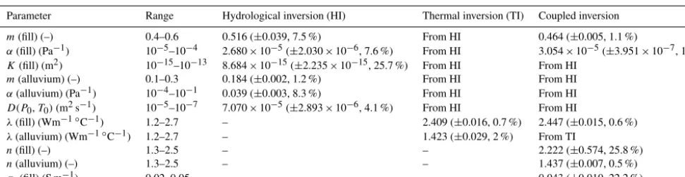
[image:8.612.52.284.65.340.2]Table 1.Constraints and estimated values of the hydrological-thermal and petrophysical parameters for different inversion cases. Hydrolog-ical inversion used matric potential data to estimate hydrologHydrolog-ical parameters (m(fill, alluvium),α(fill, alluvium),K(fill) andD). Thermal inversion used subsurface temperature data to estimate thermal conductivity of both fill and alluvium layers –λ(fill, alluvium). Coupled in-version used all matric potential, temperature and apparent-resistivity data to estimate parametersm(fill),α(fill),λ(fill),n(fill),n(alluvium) andσ (fill).
Parameter Range Hydrological inversion (HI) Thermal inversion (TI) Coupled inversion
m(fill) (–) 0.4–0.6 0.516 (±0.039, 7.5 %) From HI 0.464 (±0.005, 1.1 %)
α(fill) (Pa−1) 10−5–10−4 2.680×10⁻⁵(±2.030×10⁻⁶, 7.6 %) From HI 3.054×10⁻⁵(±3.951×10⁻⁷, 1.3 %)
K(fill) (m2) 10−15–10−13 8.684×10⁻¹⁵(±2.235×10⁻¹⁵, 25.7 %) From HI From HI
m(alluvium) (–) 0.1–0.3 0.184 (±0.002, 1.2 %) From HI From HI
α(alluvium) (Pa−1) 10−4–10−1 0.039 (±0.003, 8.3 %) From HI From HI
D(P0,T0)(m2s−1) 10−5–10−7 7.070×10⁻⁵(±2.893×10⁻⁶, 4.1 %) From HI From HI
λ(fill) (Wm−1◦C−1) 1.2–2.7 – 2.409 (±0.016, 0.7 %) 2.447 (±0.015, 0.6 %)
λ(alluvium) (Wm−1◦C−1) 1.2–2.7 – 1.423 (±0.029, 2 %) From TI
n(fill) (–) 1.3–2.5 – – 2.222 (±0.574, 25.8 %)
n(alluvium) (–) 1.3–2.5 – – 1.437 (±0.007, 0.5 %)
σs(fill) (S m−1) 0.02–0.05 – – 0.043 (±0.010, 22.2 %)
mandαrepresent the pore size distribution of the soil and reciprocal of the air-entry pressure (Eq. 7).Kis the absolute permeability (Eq. 5).D(P0,T0)is the gas diffusion coefficient at the standard condition
(P0=1 atm andT0=0◦C) (Eq. 6).λis the thermal conductivity (Eq. 12).nandσsare the saturation index and soil surface conduction, respectively (Eq. 13).
those of the alluvium layer. The |EE| of all hydrological-thermal parameters of the alluvium layer is mostly equal to 0. This is because moisture and temperature exhibit larger variations in the fill than in the alluvium layer.
3.2.2 Inversion results
The estimated parameters and their associated uncertainties based on hydrological, thermal and coupled hydrological-thermal-geophysical inversions are presented in Table 1. For the hydrological inversion, we used the matric potential data to estimate six hydrological parameters:α(both fill and allu-vium), m(both fill and alluvium), K (fill), andD(P0,T0).
Because the matric potential data are negligibly sensitive with the permeability of the alluvium layer (K (alluvium)), we did not considerK (alluvium) in hydrological inversion. We set it at 7.95×10⁻¹²m2, which is the value averaged from well measurements. For the thermal inversion, we es-timated the thermal conductivity (λ) of the fill and alluvium layers using temperature data. The specific heat capacity of the soil/sediment particles of both fill and alluvium layers was fixed at their typical value,CR=870 kg−1C−1
(Camp-bell and Norman, 1998). For the coupled hydrological-thermal-geophysical inversion, we estimated six parameters including three hydrological-thermal parameters – m (fill),
α (fill) and λ(fill) – and three petrophysical parameters,n
(both fill and alluvium) and σs (fill), using the matric
po-tential, temperature and apparent-resistivity data. The sur-face conduction of the alluvium layer was set to 0. Be-cause the apparent-resistivity data show little sensitivity to the hydrological-thermal parameters of the alluvium layer, these parameters are not improved by the coupled inversion. Therefore, they were fixed at the values obtained from the hydrological and thermal inversion. The initial guesses for the fill hydrological-thermal parameters were obtained from the previous hydrological and thermal inversion.
The hydrological inversion reveals that, compared to the other hydrological parameters, the uncertainty of the abso-lute permeability (K) of the fill layer is highest, while that of the parametermof the alluvium layer is lowest. Their stan-dard deviation are, respectively, equal to 26 and 1 % of the corresponding estimated values. It is because the matric po-tential data exhibit the lowest sensitivity withK(fill) and the highest sensitivity with m(alluvium) (see Fig. 4). Table 1 also shows that the parametersαandKof the fill layer are small, implying that this layer has a strong water-holding ca-pacity, and water will move downward slowly.
Results of the thermal inversion show that the uncertain-ties of the thermal conductivity (λ) of both fill and alluvium layers are small. This indicates that the thermal-conductivity parameter is reliably estimated, due to the dense subsurface temperature measurements and the high sensitivity of tem-perature to the parameter. Table 1 also shows that the ther-mal conductivity of both fill and alluvium layers is relatively high, which means that the variations of the temperature at the land surface are rapidly propagated downward. The ther-mal conductivity of the alluvium layer is lower than that of the fill layer. This is because a large part of the alluvium layer is saturated with water and thus has much lower thermal con-ductivity than the drier fill layer.
significantly large (26 and 22 % of the estimated values, re-spectively). This can be explained by the fact that the sat-uration index (n) and soil/sediment surface conduction (σs)
closely correlate (see Eq. 13). As a result, when both of these parameters of the fill layer are concurrently estimated, their uncertainties are higher than in the case of the alluvium layer, where only the saturation index is estimated (the surface con-duction of the alluvium was fixed atσs=0 S m−1).
Comparison of the measured and modeled matric potential of all eight datasets is presented in Fig. 5. The figure shows that there is good agreement between measured and modeled data, with a Nash–Sutcliffe efficiency criterion of 0.92. We also observe that the temporal variations of the matric poten-tial over the simulation period mostly occur at the fill layer (z≤1.5 m). When the depth is equal to or greater than 2 m, the matric potential is nearly constant. This suggests that the moisture of the alluvium layer is less dynamic, and the vari-ations within the fill layer do not frequently propagate to the alluvium layer during the simulation period.
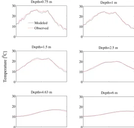
The modeled and measured temperatures at depths from 0.75 to 6 m are shown in Fig. 6. The figure indicates the model is capable of reproducing the spatial and temporal variations of the subsurface temperature. The Nash–Sutcliffe efficiency criterion is equal to 0.98. The figure also shows that at the upper depths (0.75 and 1 m) the model slightly underestimates the measurement. This can be explained by the errors of simplification at the land surface boundary. The heat and energy exchanges at the land surface between the atmosphere and land surface were not fully considered. In-stead, the land surface temperature was approximated based on the historical data of atmospheric and land surface temper-ature (see the Supplement). The evaporation was represented by the upward flux from the land surface to the atmosphere. The figure also shows that the temporal variation of the measured and modeled temperature data decrease with in-creasing depth. For example, while the temperature at depth
z=0.75 m varies in a range 8–27◦C during the simulation period, it only varies from 11 to 16◦C at depthz=6 m. The peaks of the subsurface temperature appear later at deeper locations, as it takes time for heat to flow down.
[image:10.612.310.547.63.336.2]The measured and modeled apparent-resistivity data on 8 May 2013 (when the modeled data were obtained through inversion) are depicted in Fig. 7a. The figure indicates that the coupled hydrological-thermal-geophysical simulation ef-fectively reproduces the measured data. Particularly, the lat-eral variation of the apparent resistivity is simulated with high accuracy. Both measured and modeled data clearly indi-cate that the upper part of the subsurface section is more con-ductive (lower resistivity) than the deeper part. This is rea-sonable, as the deeper section contains more sand and cob-bles, while the upper section contains more clayey and silty soils and therefore is more electrically conductive. Compar-ison of the measured and modeled resistivity data obtained from the whole simulation period is presented in Fig. 7b. The Nash–Sutcliffe efficiency criterion is equal to 0.94. Both
Figure 5.Comparison of the measured and modeled matric poten-tial data for all measurement occasions. The red symbols repre-sents the modeling results obtained from the coupled hydrological-thermal-geophysical inversion. The blue symbols denote the mea-surements.
Fig. 7a and b indicate that the estimation is less accurate for the high apparent-resistivity values. This can be explained by the fact that the high apparent-resistivity values are more sen-sitive to deeper locations and thus are harder to fit due to the influence of above soil. Another possible reason is that, with the same relative measurement error (5 %), the measurement error variances of the high resistivity values are larger than those of low resistivity values. As a result, their weights in the objective function (Eq. 15) are smaller, and they are less accurately estimated.
Figure 6.Comparison of the measured and modeled temperatures at depths of 0.75, 1, 1.5, 2.5, 4.63 and 6 m during the simulation period. The black line denotes the modeling results obtained from the coupled hydrological-thermal-geophysical inversion. The red line represents the measurements.
Figure 7.Left panels: an example of “quantitative” plots of the modeled and measured apparent-resistivity data on 8 May 2013. Right panel: comparison of all measured and modeled apparent-resistivity data in a 1 : 1 plot. The modeled data were obtained from the coupled hydrological-thermal-geophysical inversion.
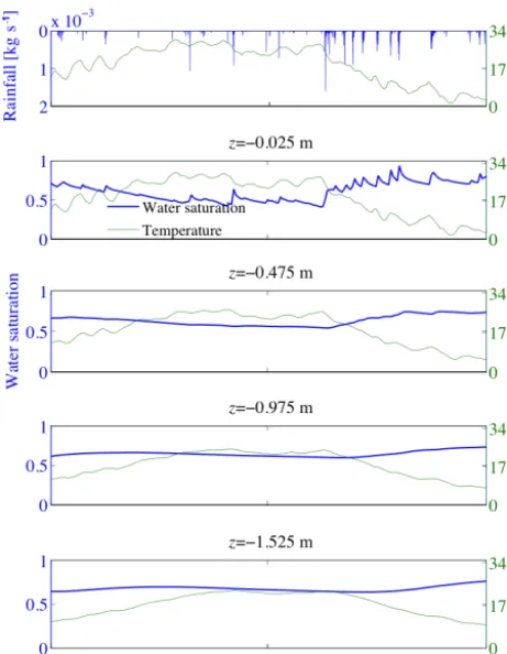
subsurface temperature exhibits a high temporal variation in a range 1.8–29.8◦C at the surface but becomes more stable at the deeper depths. At depthz=1.525 m, the temperature varies only from 9.6 to 22.2◦C.
The temporal variation of the water flux, which is the sum of the vapor and liquid fluxes versus time over the simulation period at depths from 0.025 to 1.525 m, is shown in Fig. 9. Comparing Figs. 8 and 9, we observe that the temporal vari-ation of the water flux is highly correlated with that of the water saturation and temperature. The greatest variation oc-curs at z=0.025 m, with the flux ranging from−0.001 to 0.024 m day−1. Atz=1.525 m, the flux is constantly equal to 0. The figure also indicates that the infiltration (positive
flux values) is observed at the beginning and the end of the simulation period, when the soil is wet and rainfall occurs. At the middle of the simulation period, when the air temperature is high, the upward flux (negative flux values) occurs because of evaporation. Under the control of the diffusion, the evapo-ration can lead to upward flow starting at 1 m depth.
[image:11.612.158.440.389.499.2]Figure 8.Temporal variation of the simulated water saturation and temperature at depthsz=0.025, 0.475, 0.975 and 1.525 m of the TT02 well (center of the computational domain). For reference, rainfall and soil surface temperature data are also plotted.
length, anisotropy value, variance) of these variogram func-tions as proposed in Finsterle and Kowalsky (2007).
4 Effect of temperature dependence of resistivity on hydrogeophysical inversion
[image:12.612.310.546.68.196.2]In this section, we consider the effects of the temperature dependence of the electrical resistivity on the estimated sub-surface hydrological parameters, which are obtained by in-verting apparent-resistivity data in synthetic isothermal and nonisothermal scenarios. For the isothermal scenario, the temperature was assumed to be constant in time and space at the value averaged over the whole computational do-main and over the simulation period. For the nonisother-mal scenario, the spatial and temporal variability of the tem-perature under the influences of the atmospheric tempera-ture and hydrological-thermal parameters was fully consid-ered. It is worth noting that the influences of temperature variability on the electrical resistivity include both direct (temperature–electrical-resistivity relationship) and indirect (via changing the hydrological-thermal processes, e.g., gas– liquid phase transition) effects. The synthetic experiment was implemented as below:
Figure 9.Temporal variation of the simulated water flux at depths
z=0.025, 0.475, 0.975 and 1.525 m of the TT02 well. The positive and negative values indicate the downward and upward flows.
1. Run nonisothermal hydrological-thermal-geophysical forward simulation to generate artificial apparent-resistivity data. Add Gaussian white noise (mean of 0 and standard deviation of 5 % of artificial apparent-resistivity data) to the artificial data to obtain the syn-thetic data.
2. Invert the synthetic apparent-resistivity data to estimate the subsurface hydrological parameters, assuming that the subsurface temperature is spatiotemporally constant (isothermal scenario).
3. Invert the synthetic apparent-resistivity data to estimate the subsurface hydrological parameters considering the nonisothermal process (nonisothermal scenario). 4. Compare inversion results of the two scenarios to
eval-uate the effect of the subsurface temperature variability on the hydrogeophysical inversion.
The computational domain, model parameters, and initial and boundary conditions for the synthetic forward simu-lation were taken from the coupled hydrological-thermal-geophysical inversion as presented in Section 3. Because the variation of the water saturation mostly occurs in the fill layer, we focused on estimating the hydrological pa-rameters of this layer, includingα,mand absolute perme-ability K. For both isothermal and nonisothermal scenar-ios, the initial guesses for the three parameters were set atα=1.8×10⁻⁵(Pa−1),m=0.4 andK=4.5×10⁻¹⁵m2. To increase the sensitivity of the apparent-resistivity data with the hydrological parameters, we selected four synthetic apparent-resistivity datasets corresponding with high water saturation values. The Gaussian noise, with a mean of 0 and a relative standard deviation of 5 %, was added to the arti-ficial apparent-resistivity data to generate synthetic data for the hydrogeophysical inversion.
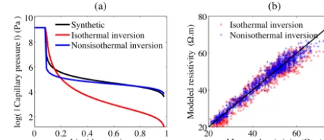
Fig. 10a. Although the nonisothermal hydrogeophysical in-version does not perfectly estimate the synthetic parameters (due to the nonuniqueness and the correlation between pa-rameters), its estimation is close to the synthetic ones. Mean-while there is a large difference between the synthetic and estimated curves obtained by the isothermal hydrogeophysi-cal scenario.
Figure 10b presents the synthetic and modeled apparent-resistivity data using a 1 : 1 plot. The figure shows that the nonisothermal scenario better reproduces the synthetic apparent resistivity than the isothermal does. Correlation, bias and root mean square error (RMSE) between the syn-thetic and simulated nonisothermal electrical resistivity data are 0.98, 1 and 2.29, respectively, while these criteria for the isothermal scenario are 0.96, 0.98 and 3.54. In brief, ignoring temperature variability and its influence on electrical resistiv-ity in the hydrogeophysical inversion is very likely to cause a large error for the model parameter estimation and to reduce agreement between modeled and measured geophysical data.
5 Summary and discussion
We developed a coupled hydrological-thermal-geophysical inversion scheme that quantifies the dependence of the elec-trical resistivity on both subsurface moisture and temper-ature, instead of solely moisture, as has been typical for previous hydrogeophysical inversion schemes. This scheme permits simulation of nonisothermal, multiphase subsurface heat and water fluxes, as well as the relationship between temperature, moisture and electrical resistivity. It accounts for the spatiotemporal variability of moisture and tempera-ture in the shallow subsurface and can include multiple geo-physical and non-geogeo-physical measurement constraints. At present, TOUGH2 cannot simulate the land surface processes and energy balance at the land surface. To mitigate this disad-vantage, this study approximated the top land surface temper-ature boundary condition from the atmospheric tempertemper-ature using a regression approach. The evaporation was considered via the gas phase of moisture. The evaporation rate was sim-ulated as the water vapor fluxes moving upward from the top layer to the atmosphere.
The new approach was applied to data collected at a field site in Rifle, Colorado. The ERT data were used to char-acterize subsurface stratigraphy and to constrain the com-putational domain for the hydrological-thermal model. The time-lapse ERT data were used with other hydrological and thermal data to constrain the inversion. The inversion results show that our developed scheme well reproduces the matric potential, temperature and apparent-resistivity data. The ob-tained results indicate that the temporal variation of the mois-ture mostly occurs at the overlying fill layer, due to the rel-atively small amount of rainfall and the high water-holding capacity of this layer. The alluvium moisture exhibits a min-imal change. Both fill and alluvium layers have high thermal
Figure 10. (a) Comparison of the synthetic and estimated van Genuchten’s retention curve.(b)Comparison of synthetic and modeled apparent-resistivity data. The red color represents the re-sults obtained by the isothermal hydrogeophysical inversion scenar-ios. The blue color denotes the nonisothermal scenario.
diffusivities, permitting the variation of the air temperature to rapidly move down. The obtained results also indicate that the thermal-conductivity and van Genuchten parameters of both fill and alluvium layers are well estimated with low un-certainties. However, due to limited temporal variations of moisture content (and thus ERT data), it is difficult to obtain the absolute permeability of the fill layer and the petrophysi-cal parameters.
To evaluate the influence of the temperature dependence of the electrical resistivity on the estimation of the hydrological parameters in the hydrogeophysical inversion, we performed a synthetic study. By comparing the results obtained from the isothermal and nonisothermal scenarios, we determined that ignoring the spatial and temporal variability of the subsurface temperature may cause errors in the estimation of hydrolog-ical parameters.
Our study documents the value of accounting for the de-pendence of both moisture content and temperature on elec-trical resistivity within a hydrological-thermal-geophysical inversion framework. The inversion scheme presented here can be widely applied to many studies striving to quantify hydrological and thermal dynamics in the subsurface. We be-lieve that this and other approaches (e.g., Kalman ensemble filter, maximum likelihood ensemble filter, particle filter) that permit rapid assimilation of autonomous monitoring datasets will greatly improve our understanding of terrestrial system properties and their behavior, including their response to en-vironmental perturbations such as floods and droughts.
6 Data availability
Both the data and input files necessary to reproduce the studies are available from the authors upon request ([email protected]).
and Environmental Research under award number DE-AC02-05CH11231. The authors would like to thank Stefan Finsterle for providing iTOUGH2 codes and support, and Thomas Günther for providing the BERT codes.
Edited by: N. Romano
Reviewed by: N. Linde and J. Boaga
References
Archie, G. E.: The electrical resistivity log as an aid in determining some reservoir characteristics, Petrol. Trans. AIME, 146, 54–62, 1942.
Arora, B., Spycher, N. F., Steefel, C. I., Molins, S., Bill, M., Con-rad, M. E., Dong, W., Faybishenko, B., Tokunaga, T. K., Wan, J., and Williams, K. H.: Influence of hydrological, biogeochemical and temperature transients on subsurface carbon fluxes in a flood plain environment, Biogeochemistry, 127, 367–396, 2016. Binley, A. and Kemna, A.: Dc resistivity and induced polarization
methods, in: Hydrogeophysics, Water Science and Technology Library, vol. 50, edited by: Rubin, Y. and Hubbard, S., Springer Netherlands, 129–156, 2005.
Binley, A., Cassiani, G., Middleton, R., and Winship, P.: Va-dose zone flow model parameterisation using cross-borehole radar and resistivity imaging, J. Hydrol., 267, 147–159, doi:10.1016/S0022-1694(02)00146-4, 2002.
Binley, A., Hubbard, S. S., Huisman, J. A., Revil, A., Robinson, D. A., Singha, K., and Slater, L. D.: The emergence of hydro-geophysics for improved understanding of subsurface processes over multiple scales, Water Resour. Res., 51, 3837–3866, 2015. Boone, R. D., Nadelhoffer, K. J., Canary, J. D., and Kaye, J. P.:
Roots exert a strong influence on the temperature sensitivity of soil respiration, Nature, 396, 570–572, doi:10.1038/25119, 1998. Brocca, L., Melone, F., Moramarco, T., Wagner, W., Naeimi, V., Bartalis, Z., and Hasenauer, S.: Improving runoff prediction through the assimilation of the ASCAT soil moisture product, Hydrol. Earth Syst. Sci., 14, 1881–1893, doi:10.5194/hess-14-1881-2010, 2010.
Campbell, G. S. and Norman, J. M.: An introduction to environmen-tal biophysics, Springer Science & Business Media, New York, USA, 1998.
Chen, J., Hubbard, S. S., and Williams, K. H.: Data-driven approach to identify field-scale biogeochemical transitions using geochem-ical and geophysgeochem-ical data and hidden Markov models: Develop-ment and application at a uranium-contaminated aquifer, Water Resour. Res., 49, 6412–6424, 2013.
Corey, A. T.: The interrelation between gas and oil relative perme-abilities, Producers Monthly, 19, 38–41, 1954.
Dafflon, B. and Barrash, W.: Three-dimensional stochastic es-timation of porosity distribution: Benefits of using ground-penetrating radar velocity tomograms in simulated-annealing-based or Bayesian sequential simulation approaches, Water Re-sour. Res., 48, W05553, doi:10.1029/2011WR010916, 2012. Day-Lewis, F. D. and Lane, J. W.: Assessing the
resolution-dependent utility of tomograms for geostatistics, Geophys. Res. Lett., 31, L07503, doi:10.1029/2004GL019617, 2004.
Doetsch, J., Linde, N., Coscia, I., Greenhalgh, S. A., and Green, A. G.: Zonation for 3D aquifer characterization based on joint
inver-sions of multimethod crosshole geophysical data, Geophysics, 75, G53–G64, doi:10.1190/1.3496476, 2010.
Finsterle, S.: iTOUGH2 User’s Guide, Lawrence Berkeley National Laboratory, Berkeley, CA, 1999.
Finsterle, S. and Kowalsky, M. B.: iTOUGH2-GSLIB user’s guide, Technical report, Lawrence Berkeley National Laboratory, Berkeley, USA, 2007.
Finsterle, S., Kowalsky, M., and Pruess, K.: TOUGH: Model use, calibration and validation, T. ASABE, 55, 1275–1290, 2012. Günther, T., Rücker, C., and Spitzer, K.: Three-dimensional
mod-elling and inversion of dc resistivity data incorporating to-pography – II. Inversion, Geophys. J. Int., 166, 506–517, doi:10.1111/j.1365-246X.2006.03011.x, 2006.
Hayley, K., Bentley, L. R., Gharibi, M., and Nightingale, M.: Low temperature dependence of electrical resistivity: Implications for near surface geophysical monitoring, Geophys. Res. Lett., 34, L18402, doi:10.1029/2007GL031124, 2007.
Hayley, K., Bentley, L., and Pidlisecky, A.: Compensating for tem-perature variations in time-lapse electrical resistivity difference imaging, Geophysics, 75, WA51–WA59, 2010.
Hubbard, S. S. and Linde, N.: Hydrogeophysics, in: Chapter 43, Treatise on Water, edited by: Wilderer, P., Elsevier, Amsterdam, the Netherlands, 2011.
Hubbard, S. S., Chen, J., Peterson, J., Majer, E. L., Williams, K. H., Swift, D. J., Mailloux, B., and Rubin, Y.: Hydrogeologi-cal characterization of the south oyster bacterial transport site using geophysical data, Water Resour. Res., 37, 2431–2456, doi:10.1029/2001WR000279, 2001.
Hubbard, S. S., Gangodagamage, C., Dafflon, B., Wainwright, H., Peterson, J., Gusmeroli, A., Ulrich, C., Wu, Y., Wilson, C., Row-land, J. and Tweedie, C.: Quantifying and relating land-surface and subsurface variability in permafrost environments using Li-dar and surface geophysical datasets, Hydrogeol. J., 21, 149–169, 2013.
Huisman, J., Rings, J., Vrugt, J., Sorg, J., and Vereecken, H.: Hy-draulic properties of a model dike from coupled Bayesian and multi-criteria hydrogeophysical inversion, J. Hydrol., 380, 62– 73, doi:10.1016/j.jhydrol.2009.10.023, 2010.
Johnson, T. C., Versteeg, R. J., Huang, H., and Routh, P. S.: Data-domain correlation approach for joint hydrogeologic inversion of time-lapse hydrogeologic and geophysical data, Geophysics, 74, F127–F140, 2009.
Kemna, A., Vanderborght, J., Kulessa, B., and Vereecken, H.: Imag-ing and characterisation of subsurface solute transport usImag-ing electrical resistivity tomography (ERT) and equivalent transport models, J. Hydrol., 267, 125–146, 2002.
Kowalsky, M. B., Finsterle, S., Peterson, J., Hubbard, S. S., Rubin, Y., Majer, E., Ward, A., and Gee, G.: Estimation of field-scale soil hydraulic and dielectric parameters through joint inversion of GPR and hydrological data, Water Resour. Res., 41, W11425, doi:10.1029/2005WR004237, 2005.
Kowalsky, M. B., Gasperikova, E., Finsterle, S., Watson, D., Baker, G., and Hubbard, S. S.: Coupled modeling of hydrogeochemical and electrical resistivity data for exploring the impact of recharge on subsurface contamination, Water Resour. Res., 47, W02509, doi:10.1029/2009WR008947, 2011.
inversion of time-Lapse, off-ground GPR data, Vadose Zone J., 8, 743–754, 2009.
Li, L., Steefel, C. I., Kowalsky, M. B., Englert, A., and Hubbard, S. S.: Effects of physical and geochemical heterogeneities on min-eral transformation and biomass accumulation during biostimu-lation experiments at Rifle, Colorado, J. Contam. Hydrol., 112, 45–63, 2010.
Linde, N., Binley, A., Tryggvason, A., Pedersen, L. B., and Revil, A.: Improved hydrogeophysical characterization using joint inversion of cross-hole electrical resistance and ground-penetrating radar traveltime data, Water Resour. Res., 42, W12404, doi:10.1029/2006WR005131, 2016.
Llera, F. J., Sato, M., Nakatsuka, K., and Yokoyama, H.: Temper-ature dependence of the electrical resistivity of water-saturated rocks, Geophysics, 55, 576–585, doi:10.1190/1.1442869, 1990. Luo, G. J., Kiese, R., Wolf, B., and Butterbach-Bahl, K.: Effects
of soil temperature and moisture on methane uptake and nitrous oxide emissions across three different ecosystem types, Biogeo-sciences, 10, 3205–3219, doi:10.5194/bg-10-3205-2013, 2013. Ma, Y., Van Dam, R. L., and Jayawickreme, D. H.: Soil moisture
variability in a temperate deciduous forest: insights from electri-cal resistivity and throughfall data, Environ. Earth Sci., 72, 1367– 1381, doi:10.1007/s12665-014-3362-y, 2014.
Marquardt, D. W.: An algorithm for least-squares estimation of nonlinear parameters, J. Soc. Indust. Appl. Math., 11, 431–441, 1963.
McClymont, A. F., Hayashi, M., Bentley, L. R., and Chris-tensen, B. S.: Geophysical imaging and thermal modeling of subsurface morphology and thaw evolution of discontinu-ous permafrost, J. Geophys. Res.-Ea. Surf., 118, 1826–1837, doi:10.1002/jgrf.20114, 2013.
Merz, B. and Bardossy, A.: Effect of spatial variability on the rain-fall runoff process in a small loess catchment, J. Hydrol., 212, 304–317, 1998.
Morris, M. D.: Factorial sampling plans for preliminary computational experiments, Technometrics, 33, 161–174, doi:10.1080/00401706.1991.10484804, 1991.
Musgrave, H. and Binley, A.: Revealing the temporal
dy-namics of subsurface temperature in a wetland
us-ing time-lapse geophysics, J. Hydrol., 396, 258–266, doi:10.1016/j.jhydrol.2010.11.008, 2011.
Pruess, K., Oldenburg, C., and Moridis, G.: TOUGH2 user’s guide, version 2.0, Lawrence Berkeley National Laboratory, Berkeley, CA, 1999.
Rein, A., Hoffmann, R., and Dietrich, P.: Influence of nat-ural time-dependent variations of electrical conductivity on DC resistivity measurements, J. Hydrol., 285, 215–232, doi:10.1016/j.jhydrol.2003.08.015, 2004.
Revil, A., Karaoulis, M., Johnson, T., and Kemna, A.: Review: Some low-frequency electrical methods for subsurface character-ization and monitoring in hydrogeology, Hydrogeol. J., 20, 617– 658, doi:10.1007/s10040-011-0819-x, 2012.
Rodriguez-Iturbe, I.: Ecohydrology: A hydrologic perspective of climate-soil-vegetation dynamics, Water Resour. Res., 36, 3–9, doi:10.1029/1999WR900210, 2000.
Rubin, Y. and Hubbard, S. S.: Hydrogeophysics, vol. 50, Springer, the Netherlands, 2005.
Rücker, C., Gunther, T., and Spitzer, K.: Three-dimensional mod-elling and inversion of DC resistivity data incorporating to-pography – I. modelling, Geophys. J. Int., 166, 495–505, doi:10.1111/j.1365-246X.2006.03010.x, 2006.
Sen, P. and Goode, P.: Influence of temperature on electri-cal conductivity on shaly sands, Geophysics, 57, 89–96, doi:10.1190/1.1443191, 1992.
Singha, K. and Gorelick, S. M.: Saline tracer visualized with three-dimensional electrical resistivity tomography: Field-scale spatial moment analysis, Water Resour. Res., 41, W05023, doi:10.1029/2004WR003460, 2005.
Tran, A. P., Vanclooster, M., Zupanski, M., and Lambot, S.: Joint estimation of soil moisture profile and hydraulic parameters by ground-penetrating radar data assimilation with maximum likelihood ensemble filter, Water Resour. Res., 50, 3131–3146, doi:10.1002/2013WR014583, 2014.
Tran, A. P., Bogaert, P., Wiaux, F., Vanclooster, M., and Lambot, S.: High-resolution space–time quantification of soil moisture along a hillslope using joint analysis of ground penetrating radar and frequency domain reflectometry data, J. Hydrol., 523, 252–261, 2015.
Tran, A. P., Dafflon, B., and Hubbard, S.: iMatTOUGH: An open-source Matlab-based graphical user interface for pre- and post-processing of TOUGH2 and iTOUGH2 models, Comput. Geosci., 89, 132–143, doi:10.1016/j.cageo.2016.02.006, 2016. van Genuchten, M. T.: A closed-form equation for predicting the
hydraulic conductivity of unsaturated soils, Soil Sci. Soc. Am. J., 44, 892–898, 1980.
Wainwright, H. M., Finsterle, S., Jung, Y., Zhou, Q., and Birkholzer, J. T.: Making sense of global sensitivity analyses, Comput. Geosci., 65, 84–94, doi:10.1016/j.cageo.2013.06.006, 2013. Wainwright, H. M., Orozco, A. F., Bücker, M., Dafflon, B.,
Chen, J., Hubbard, S. S., and Williams, K. H.: Hierarchical Bayesian method for mapping biogeochemical hot spots using induced polarization imaging, Water Resour. Res., 52, 533–551, doi:10.1002/2015WR017763, 2015.
Yabusaki, S. B., Fang, Y., Williams, K. H., Murray, C. J., Ward, A. L., Dayvault, R. D., Waichler, S. R., Newcomer, D. R., Spane, F. A., and Long, P. E.: Variably saturated flow and multicomponent biogeochemical reactive transport modeling of a uranium biore-mediation field experiment, J. Contam. Hydrol., 126, 271–290, 2011.