Flood risk reduction and flow buffering as ecosystem services – Part 2: Land use and rainfall intensity effects in Southeast Asia

Hydrol. Earth Syst. Sci., 21, 2341–2360, 2017 www.hydrol-earth-syst-sci.net/21/2341/2017/ doi:10.5194/hess-21-2341-2017

© Author(s) 2017. CC Attribution 3.0 License.

Flood risk reduction and flow buffering as ecosystem services –

Part 2: Land use and rainfall intensity effects in Southeast Asia

Meine van Noordwijk1,2, Lisa Tanika1, and Betha Lusiana1

1_{World Agroforestry Centre, Bogor, Indonesia}

2_{Plant Production System, Wageningen University, Wageningen, the Netherlands} Correspondence to:Meine van Noordwijk ([email protected])

Received: 15 December 2015 – Discussion started: 19 January 2016 Revised: 24 March 2017 – Accepted: 4 April 2017 – Published: 5 May 2017

Abstract. Watersheds buffer the temporal pattern of river flow relative to the temporal pattern of rainfall. This “ecosys-tem service” is inherent to geology and climate, but buffer-ing also responds to human use and misuse of the land-scape. Buffering can be part of management feedback loops if salient, credible and legitimate indicators are used. The flow persistence parameter Fp in a parsimonious recursive

model of river flow (Part 1, van Noordwijk et al., 2017) cou-ples the transmission of extreme rainfall events (1−Fp), to

the annual base-flow fraction of a watershed (Fp). Here we

compareFpestimates from four meso-scale watersheds in

In-donesia (Cidanau, Way Besai and Bialo) and Thailand (Mae Chaem), with varying climate, geology and land cover his-tory, at a decadal timescale. The likely response in each of these four to variation in rainfall properties (including the maximum hourly rainfall intensity) and land cover (compar-ing scenarios with either more or less forest and tree cover than the current situation) was explored through a basic daily water-balance model, GenRiver. This model was calibrated for each site on existing data, before being used for alterna-tive land cover and rainfall parameter settings. In both data and model runs, the wet-season (3-monthly)Fpvalues were

consistently lower than dry-season values for all four sites. Across the four catchmentsFpvalues decreased with

increas-ing annual rainfall, but specific aspects of watersheds, such as the riparian swamp (peat soils) in Cidanau reduced effects of land use change in the upper watershed. Increasing the mean rainfall intensity (at constant monthly totals for rain-fall) around the values considered typical for each landscape was predicted to cause a decrease in Fpvalues by between

0.047 (Bialo) and 0.261 (Mae Chaem). Sensitivity of Fpto

changes in land use change plus changes in rainfall intensity

depends on other characteristics of the watersheds, and gen-eralisations made on the basis of one or two case studies may not hold, even within the same climatic zone. A wet-season

Fpvalue above 0.7 was achievable in forest–agroforestry

mo-saic case studies. Inter-annual variability inFpis large

rela-tive to effects of land cover change. Multiple (5–10) years of paired-plot data would generally be needed to reject no-change null hypotheses on the effects of land use no-change (degradation and restoration).Fp trends over time serve as

a holistic scale-dependent performance indicator of degrad-ing/recovering watershed health and can be tested for accept-ability and acceptance in a wider social-ecological context.

1 Introduction

the other side of the spectrum, river flow can be constant ev-ery day, beyond the theoretical condition of constant rainfall, in a watershed that provides perfect buffering, by passing all water through groundwater pools that have sufficient storage capacity at any time during the year. Both infiltration-limited (Hortonian) and saturation-induced use of more rapid flow pathways (inter and overland flows) will reduce the flow per-sistence and make it, at least in part, dependent on rainfall events. Separating the effects of land cover (land use), en-gineering and rainfall on the actual flow patterns of rivers remains a considerable challenge (Ma et al., 2014; Verbist et al., 2010). It requires data, models and concepts that can serve as an effective boundary object in communication with stakeholders (Leimona et al., 2015; van Noordwijk et al., 2012, 2016). There is a long tradition in using forest cover as such a boundary object, but there is only a small amount of evidence supporting this (Tan-Soo et al., 2016; van Dijk et al., 2009; van Noordwijk et al., 2015a).

In Part 1 (van Noordwijk et al., 2017), we introduced a flow persistence parameter (Fp) that links the two,

asymmet-rical aspects of flow dynamics: translating rainfall excess into river flow, and gradually releasing water stored in the land-scape. The direct link between these two aspects can be seen from Eq. (4) in Part 1 (van Noordwijk et al., 2017):

Qt=FpQt−1+ 1−Fp

(Pt−Et x) , (1)

whereQt andQt−1represent river flow on subsequent days, Pt xthe precipitation on dayt(or preceding precipitation re-leased as snowmelt on dayt) andEt x the preceding evapo-transpiration since the previous precipitation event, creating storage space in the soils of the watershed. The first term on the right-hand side of the equation represents the gradual re-lease of stored water, causing a slow decline of flow as the pools feeding this flow are gradually depleted. The second term reflects the part of fresh additions of water are parti-tioned over immediate river flow and the increase of stocks from which water can be gradually released. The derivation of the link depended on the long-term water balance, and thus assumed that all out- and inflows are accounted for in the wa-tershed.

Commonly used rainfall–runoff models (including the curve number approach and SWAT models) only focus on the second term of the above equation (Ponce et al., 1996; Gassman et al., 2007), without link to the first. Various em-pirical methods for deriving “base flow” are in use, but de-tails of the calculation procedure matter. Results in Part 1 (van Noordwijk et al., 2017) for a number of contrast-ing meso-scale watersheds in Southeast Asia suggested that inter-annual variation inFpwithin a given watershed

corre-lates with both the Richards–Baker (R–B) flashiness index (Baker et al., 2004) and the base-flow fraction of annual river flow. However, the slope of these relationships varied be-tween watersheds. Here, in Part 2 we will further analyse the

Fpresults for these watersheds that were selected to

repre-sent variation in rainfall and land cover, and test the internal

consistency of results based on historical data: two located in the humid and one in the subhumid tropics of Indonesia, and one in the unimodal subhumid tropics of northern Thailand.

After exploring the patterns of variation inFpestimates

derived from actual river flow records, we will quantify the sensitivity of the Fp metric to variations in rainfall

inten-sity and its response, on a longer timescale to land cover change. To do so, we will use a model that uses basic water-balance concepts: rainfall interception, infiltration, water use by vegetation, overland flow, interflow and groundwater re-lease, to a spatially structured watershed where travel time from sub-watersheds to any point of interest modifies the pre-dicted river flow. In the specific model used, land cover ef-fects on soil conditions, interception and seasonal water use have been included. After testing whetherFpvalues derived

from model outputs match those based on empirical data where these exist, we rely on the basic logic of the model to make inference on the relative importance of modifying rainfall and land cover inputs. With the resulting temporal variation in calculatedFpvalues, we consider the time frame

at which observed shifts inFp can be attributed to factors

other than chance (i.e. null hypotheses of random effects can be rejected with accepted chance of Type I errors).

2 Methods

2.1 GenRiver model for effects of land cover on river flow

M. van Noordwijk et al.: Flood risk reduction and flow buffering as ecosystem services – Part 2 2343

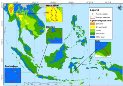
Figure 1.Location of the four watersheds in the agro-ecological zones of Southeast Asia (water towers are defined on the basis of its ability to generate river flow and being in the upper part of a watershed).

a coefficient of variation as parameter. For the Mae Chaem site in northern Thailand, data by Dairaku et al. (2004) sug-gested a mean of less than 3 mm h−1. For the three sites in Indonesia we used 30 mm h−1, based on Kusumastuti et al. (2016). Appendix B provides further detail on the GenRiver model. The model itself, a manual and application case stud-ies, are freely available (http://www.worldAgroforestry.org/ output/genriver-generic-river-model-river-flow; van Noord-wijk et al., 2011).

2.2 Empirical data sets, model calibration

Table 1 and Fig. 1 provide summary characteristics and the location of river flow data used in four meso-scale water-sheds for testing theFpalgorithm and application of the

Gen-River model. Figure 1 includes a water tower category in the agro-ecological zones; this is defined on the basis of a ra-tio of precipitara-tion and potential evapotranspirara-tion of more than 0.65, and a product of that ratio and relative elevation exceeding 0.277.

As major parameters for the GenRiver model were not independently measured for the respective watersheds, we tuned (calibrated) the model by modifying parameters within a predetermined plausible range, and used correspondence with measured hydrograph as test criterion (Kobold et al., 2008). We used the Nash–Sutcliffe efficiency (NSE) parame-ter (target above 0.5) and bias (less than 25 %) as test criparame-teria

and targets. Meeting these performance targets (Moriasi et al., 2007), we accepted the adjusted models as basis for de-scribing current conditions and exploring model sensitivity. The main site-specific parameter values are listed in Table 2 and (generic) land-cover-specific default parameters in Ta-ble 3.

Table 4 describes the six scenarios of land use change that were evaluated in terms of their hydrological impacts. Fur-ther description on the associated land cover distribution for each scenario in the four different watersheds is depicted in Appendix C.

2.3 Bootstrapping to estimate the minimum observation

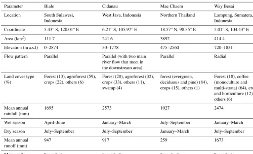
dis-Table 1.Basic physiographic characteristics of the four study watersheds.

Parameter Bialo Cidanau Mae Chaem Way Besai

Location South Sulawesi, West Java, Indonesia Northern Thailand Lampung, Sumatera,

Indonesia Indonesia

Coordinate 5.43◦S, 120.01◦E 6.21◦S, 105.97◦E 18.57◦N, 98.35◦E 5.01◦S, 104.43◦E

Area (km2) 111.7 241.6 3892 414.4

Elevation (m a.s.l) 0–2874 30–1778 475–2560 720–1831

Flow pattern Parallel Parallel (with two main Parallel Radial river flow that meet in

the downstream area)

Land cover type Forest (13), agroforest (59), Forest (20), agroforest (32), forest (evergreen, Forest (18), coffee (%) crops (22), others (6) crops (33), others (11), deciduous and pine) (84), (monoculture and

swamp (4) crops (15), others (1) multi-strata) (64), crop and horticulture (12), others (6)

Mean annual 1695 2573 1027 2474

rainfall (mm)

Wet season April–June January–March July–September January–March

Dry season July–September July–September January–March July–September

Mean annual 947 917 259 1673

runoff (mm)

Major soils Inceptisols Inceptisols Inceptisols Inceptisols

charge data (Zhang et al., 2006). We built a simple macro in R (R Core Team, 2017) that entails the following steps:

i. bootstrap or resample with replacement 1000 times from both time series discharge data with sample sizen; ii. apply the Kolmogorov–Smirnov test to each of the 1000 generated pair-wise discharge data, and record the

pvalue;

iii. perform (i) and (ii) for different size of n, ranging from 5 to 50;

iv, tabulate thep value from the different sample sizen, and determine the value ofnwhen thepvalue reached equal to or less than 0.025 (or equal to the significance level of 5 %); the associatednrepresents the minimum number of observations required.

Appendix D provides an example of the macro in R used for this analysis.

3 Results

3.1 Empirical data of flow persistence as basis for model parameterisation

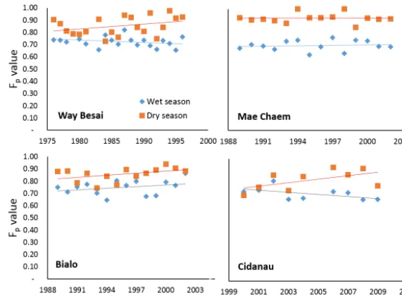
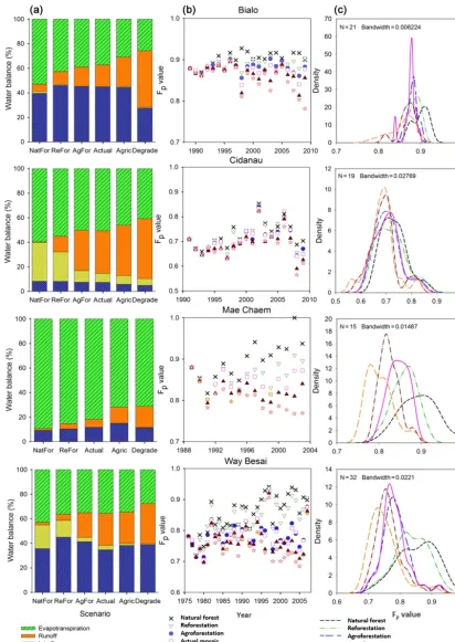
Inter-annual variability ofFpestimates derived for the four

catchments (Fig. 2) was of the order of 0.1 units, while the intra-annual variability between dry and rainy seasons was 0.1–0.2. For all years and locations, rainy-seasonFp

val-ues, with mixed flow pathways, were consistently below dry-season values, dominated by groundwater flows. If we can expectFp,i andFp,0(see Eq. 8 in Part 1, van Noordwijk et

al., 2017) to be approximately 0.5 and 0, this difference be-tween wet and dry periods implies a 40 % contribution of interflow in the wet season, a 20 % contribution of overland flow or any combination of the two effects.

Overall the estimates from modelled and observed data are related with 16 % deviating more than 0.1 and 3 % more than 0.15 (Fig. 3). As the Moriasi et al. (2007) performance criteria for the hydrographs were met by the calibrated mod-els for each site, we tentatively accept the model to be a basis for a sensitivity study ofFp to modifications to land cover

M. van Noordwijk et al.: Flood risk reduction and flow buffering as ecosystem services – Part 2 2345

Figure 2.Flow persistence (Fp) estimates derived from measurements in four Southeast Asian watersheds, separately for the wettest and driest 3-month periods of the year.

Figure 3.Inter-(a)and intra-annual(b)variation in theFpparameter derived from empirical vs. modelled flow: for the four test sites on annual basis(a)or 3-monthly basis(b).

3.2 ComparingFpeffect of rainfall intensity and land

cover change

A direct comparison of model sensitivity to changes in mean rainfall intensity and land use change scenarios is provided in Fig. 4. Varying the mean rainfall intensity over a fac-tor 7 shifted the Fp value by only 0.047 and 0.059 in the

case of Bialo and Cidanau, respectively, but by 0.128 in Way Besai and 0.261 in Mae Chaem (Fig. 4a). The impact of the land use change scenarios onFpwas the smallest in

Cidanau (0.026), intermediate in Way Besai (0.048) and rel-atively large in Bialo and Mae Chaem, at 0.080 and 0.084, respectively (Fig. 4b). The order of Fp across the land use

change scenarios was mostly consistent between the water-sheds, but the contrast between the reforestation and natural forest scenario was the largest in Mae Chaem and the

small-est in Way Besai. In Cidanau, Way Besai and Mae Chaem, variations in rainfall were 2.2 to 3.1 times more effective than land use change in shiftingFp, whereas in Bialo its relative

effect was only 58 %. Apparently, the sensitivity to changes in land use change plus changes in rainfall intensity depends on other characteristics of the watersheds, and generalisa-tions made on the basis of one or two case studies may not hold, even within the same climatic zone.

3.3 Further analysis ofFpeffects for scenarios of land

cover change

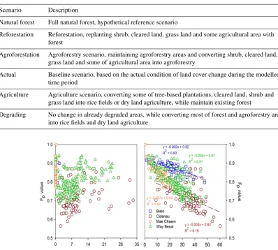
Among the four watersheds there is consistency in that the “forest” scenario has the highest, and the “degraded lands” the lowest,Fp value (Fig. 5), but there are remarkable

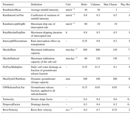
Table 2.Parameters of the GenRiver model used for the four site-specific simulations (van Noordwijk et al., 2011 for definitions of terms; sequence of parameters follows the pathway of water).

Parameter Definition Unit Bialo Cidanau Mae Chaem Way Besai

RainIntensMean Average rainfall intensity mm h−1 30 30 3 30 RainIntensCoefVar Coefficient of variation of mm h−1 0.8 0.3 0.5 0.3

rainfall intensity

RainInterceptDripRt Maximum drip rate of mm h−1 80 10 10 10 intercepted rain

RainMaxIntDripDur Maximum dripping duration h 0.8 0.5 0.5 0.5 of intercepted rain

InterceptEffectontrans Rain interception effect on – 0.35 0.8 0.3 0.8 transpiration

MaxInfRate Maximum infiltration mm day−1 580 800 150 720 capacity

MaxInfSubsoil Maximum infiltration mm day−1 80 120 150 120 capacity of the sub-soil

PerFracMultiplier Daily soil water drainage as – 0.35 0.13 0.1 0.1 fraction of groundwater

release fraction

MaxDynGrWatStore Dynamic groundwater mm 100 100 300 300 storage capacity

GWReleaseFracVar Groundwater release – 0.15 0.03 0.05 0.1 fraction, applied to all

subcatchments

Tortuosity Stream shape factor – 0.4 0.4 0.6 0.45

DispersalFactor Drainage density – 0.3 0.4 0.3 0.45

RiverVelocity River flow velocity m s−1 0.4 0.7 0.35 0.5

M. van Noordwijk et al.: Flood risk reduction and flow buffering as ecosystem services – Part 2 2347

Figure 6.Frequency distribution of expected difference inFpin “paired-plot” comparisons where land cover is the only variable; left panels: all scenarios compared to “reforestation”; right panel: all scenarios compared to degradation; graphs are based on a kernel density estimation (smoothing) approach.

Table 3.GenRiver defaults for land-use-specific parameter values, used for all four watersheds (BD/BDref indicates the bulk density relative to that for an agricultural soil pedotransfer function; see van Noordwijk et al., 2011).

Land cover type Potential Relative Bd/BDref interception drought

(mm day−1) threshold

Forest1 3.0–4.0 0.4–0.5 0.8–1.1 Agroforestry2 2.0–3.0 0.5–0.6 0.95–1.05 Monoculture tree3 1.0 0.55 1.08 Annual crops 1.0–3.0 0.6–0.7 1.1–1.5

Horticulture 1.0 0.7 1.07

Rice field4 1.0–3.0 0.9 1.1–1.2

Settlement 0.05 0.01 1.3

Shrub and grass 2.0–3.0 0.6 1.0–1.07 Cleared land 1.0–1.5 0.3–0.4 1.1–1.2

Note1forest: primary forest, secondary forest, swamp forest, evergreen forest, deciduous forest.2_{agroforest: mixed garden, clove, coffee, cocoa.}

3_{monoculture: coffee;}4_{rice field: irrigation and rainfed.}

is clearly larger than land cover effects, while in the Way Besai the spread in land use scenarios is larger than inter-annual variability. In Cidanau a peat swamp between most of the catchment and the measuring point buffers most of

land-cover-related variation in flow, but not the inter-annual variability. Considering the frequency distributions ofFp

val-ues over a 20-year period, we see one watershed (Way Besai) where the forest stands out from all others, and one (Bialo) where the degraded lands are separate from the others. Given the degree of overlap of the frequency distributions, it is clear that multiple years of empirical observations will be needed before a change can be affirmed.

Figure 5 shows the frequency distributions of expected ef-fect sizes onFp of a comparison of any land cover with

ei-ther forest or degraded lands. Table 5 translates this informa-tion to the number of years that a paired plot (in the absence of measurement error) would have to be maintained to re-ject a null hypothesis of no effect, at 5 % probability (p). As the frequency distributions ofFpdifferences of paired

statis-M. van Noordwijk et al.: Flood risk reduction and flow buffering as ecosystem services – Part 2 2349

Table 4.Land use scenarios explored for four watersheds.

Scenario Description

Natural forest Full natural forest, hypothetical reference scenario

Reforestation Reforestation, replanting shrub, cleared land, grass land and some agricultural area with forest

Agroforestation Agroforestry scenario, maintaining agroforestry areas and converting shrub, cleared land, grass land and some of agricultural area into agroforestry

Actual Baseline scenario, based on the actual condition of land cover change during the modelled time period

Agriculture Agriculture scenario, converting some of tree-based plantations, cleared land, shrub and grass land into rice fields or dry land agriculture, while maintain existing forest

Degrading No change in already degraded areas, while converting most of forest and agroforestry area into rice fields and dry land agriculture

Figure 7.Correlations ofFpwith fractions of rainfall that take overland flow and interflow pathways through the watershed, across all years and land use scenarios of Fig. App2.

tical tests will not emerge, even though effects on watershed health are real.

At process level the increase in “overland flow” in re-sponse to soil compaction due to land cover change has a clear and statistically significant relationship with decreas-ing Fp values in all catchments (Fig. 6), but both

year-to-year variation within a catchment and differences between catchments influence the results as well, leading to consider-able spread in the bi-plot. Contrary to expectations, the dis-appearance of “interflow” by soil compaction is not reflected in measurable change in Fp value. The temporal difference

between overland and interflow (1 or a few days) gets eas-ily blurred in the river response that integrates over multi-ple streams with variation in delivery times; the difference between overland- or interflow and base flow is much more pronounced. Apparently, according to our model, the high macroporosity of forest soils that allows for interflow, and may be the “sponge” effect attributed to forest, delays de-livery to rivers by 1 or a few days, with little effect on the

flow volumes at locations downstream where flow of multi-ple days accumulates. The difference between overland- or interflow and base flow in time-to-river of rainfall peaks is much more pronounced.

Table 5.Number of years of observations required to estimate flow persistence to reject the null hypothesis of “no land use effect”, at

p value=0.05 using Kolmogorov–Smirnov test. The probability of the test statistic in the first significant number is provided between brackets and where the number of observations exceeds the time series available, results are given in italics.

(a) Natural forest as reference

Way Besai (N=32) Reforestation Agroforestation Actual Agricultural Degrading Reforestation – 20 (0.0035) 16 (0.037) 13 (0.046) 11 (0.023)

Agroforestation – – n.s n.s. n.s.

Actual – – – n.s. n.s.

Agricultural – – – – n.s.

Degrading – – – – –

Bialo (N=18) Reforestation Agroforestation Actual Agricultural Degrading

Reforestation – n.s. n.s. 37 (0.04) 27 (0.040)

Agroforestation – – n.s n.s. n.s.

Actual – – – n.s. n.s.

Agricultural – – – – n.s.

Degrading – – – – –

Cidanau (N=20) Reforestation Agroforestation Actual Agricultural Degrading

Reforestation – n.s. n.s. 32 (0.037) 48 (0.043)

Agroforestation – – n.s n.s. n.s.

Actual – – – n.s. n.s.

Agricultural – – – – n.s.

Degrading – – – – –

Mae Chaem (N=15) Reforestation Actual Agricultural Degrading

Reforestation – n.s. 23 (0.049) 18 (0.050)

Actual – – 45 (0.037) 33 (0.041)

Agricultural – – – 33 (0.041)

Degrading – – – –

(b) Degrading scenario as reference

Way Besai (N=32) Natural forest Reforestation Agroforestation Actual Agricultural Natural forest – n.s. 17 (0.042) 13 (0.046) 7 (0.023) Reforestation – – 21 (0.037) 19 (0.026) 7 (0.023)

Agroforestation – – – n.s. 28 (0.046)

Actual – – – – 30 (0.029)

Agricultural – – – – –

Bialo (N=18) Natural forest Reforestation Agroforestation Actual Agricultural

Natural forest – n.s. n.s. 41 (0.047) 19 (0.026)

Reforestation – – n.s. n.s. 32 (0.037)

Agroforestation – – – n.s. n.s.

Actual – – – – n.s.

Agricultural – – – – –

Cidanau (N=20) Natural forest Reforestation Agroforestation Actual Agricultural

Natural forest – n.s. n.s. 33 (0.041) 8 (0.034)

Reforestation – – n.s. n.s. 15 (0.028)

Agroforestation – – – n.s. n.s.

Actual – – – – 25 (0.031)

Agricultural – – – – –

Mae Chaem (N=20) Natural forest Reforestation Actual Agricultural

Natural forest – n.s. 25 (0.031) 12 (0.037)

Reforestation – – n.s. 18 (0.050)

Actual – – – 18 (0.050)

M. van Noordwijk et al.: Flood risk reduction and flow buffering as ecosystem services – Part 2 2351

flow persistence are small relative to inter-annual variabil-ity due to specific rainfall patterns, and that it will be hard for any empirical data process to pickup such effects, even if they are qualitatively aligned with valid process-based mod-els.

4 Discussion

In the discussion of Part 1 (van Noordwijk et al., 2017), the credibility questions on replicability of theFpmetric and its

sensitivity to details of rainfall pattern vs. land cover as po-tential causes of variation were seen as requiring case stud-ies in a range of contexts. Although the four case studstud-ies in Southeast Asia presented here cannot be claimed to repre-sent the global variation in catchment behaviour (with ab-sence of a snowpack and its dynamics as an obvious element of flow buffering not included), the diversity of responses among these four already point to challenges for any generic interpretation of the degree of flow persistence that can be achieved under natural forest cover, as well as its response to land cover change.

Where Fig. 8 in Part 1 (van Noordwijk et al., 2017) explored the relationship in inter-annual variation between flashiness index andFpin the actual data for the four

water-sheds, we can now repeat the analysis for the modelled re-sults for each scenario. Figure 8 presents two examples with, again, evidence that the flashiness index andFpare related,

but with considerable variation between the watersheds and a lower slope for the Cidanau watershed with its downstream flow buffering.

The empirical data summarised here for (sub)humid trop-ical sites in Indonesia and Thailand show that values ofFp

above 0.9 are scarce in the case studies provided, but val-ues above 0.8 were found, or inferred by the model, for forested landscapes. Agroforestry landscapes generally pre-sented Fp values above 0.7, while open-field agriculture or

degraded soils led toFpvalues of 0.5 or lower. Due to

differ-ences in local context, it may not be feasible to relate typical

Fpvalues to the overall condition of a watershed, but

tempo-ral change inFpcan indicate degradation or restoration if a

location-specific reference can be found. The difference be-tween wet- and dry-seasonFpcan be further explored in this

context. The dry-seasonFpvalue primarily reflects the

un-derlying geology, with potential modification by engineering and operating rules of reservoirs, the wet-seasonFpis

gen-erally lower due to partial shifts to overland and interflow pathways. Where further uncertainty is introduced by the use of modelled rather than measured river flow, the lack of fit of models similar to the ones we used here would mean that sce-nario results are indicative of directions of change rather than a precision tool for fine-tuning combinations of engineering and land cover change as part of integrated watershed man-agement.

The differences in relative response of the watersheds to changes in mean rainfall intensity and land cover change suggest that generalisations derived from one or a few case studies are to be interpreted cautiously. If land cover change would influence details of the rainfall generation process (ar-row 10 in Fig. 1 of Part 1, (van Noordwijk et al., 2017); e.g. through release of ice-nucleating bacteria, (Morris et al., 2014; van Noordwijk et al., 2015b; Ellison et al., 2017) this can easily dominate over effects via interception, transpira-tion and soil changes.

Our results indicate an intra-annual variability ofFpvalues

between wet and dry seasons of around 0.2 in the case stud-ies, while inter-annual variability in either annual or seasonal

Fp was generally in the 0.1 range. The difference between

observed and simulated flow data as basis forFpcalculations

was mostly less than 0.1. With current methods, it seems that effects of land cover change on flow persistence that shift the

Fpvalue by about 0.1 are the limit of what can be asserted

from empirical data (with shifts of that order in a single year a warning sign rather than a firmly established change). When derived from observed river flow data,Fpis suitable for

mon-itoring change (degradation, restoration) and can be a seri-ous candidate for monitoring performance in outcome-based ecosystem service management contracts. Choice of the part of the year for whichFpchanges are used as indicator may

have to depend on the seasonal patterns of rainfall.

In view of our results, the lack of robust evidence in the literature of effects of change in forest and tree cover on flood occurrence may not be a surprise; effects are subtle and most data sets contain considerable variability. Yet, such effects are consistent with current process and scaling knowledge of watersheds.

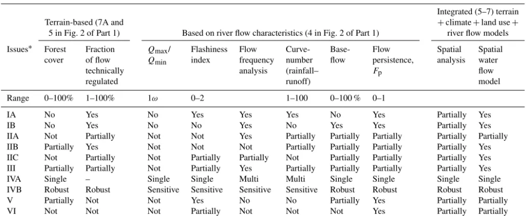
In summarising findings on theFp metric, we can

com-pare it with existing ones across the seven questions raised in Fig. 1 of Part 1 (van Noordwijk et al., 2017). Compara-tor metrics can be derived from various data sources, includ-ing the amount (and/or quality) of forest cover upstream, the fraction of flows that is technically controlled, direct records of river flow (over a short or longer time period), records of rainfall and/or models that combine landscape properties, climate and land cover. Tentative scoring for these metrics (Table 6) suggests that theFpmetric is an efficient tool for

data-scarce environments, as it indicates aspects of hydro-graphs that so far required multi-annual records of river flow.

5 Conclusions

Figure 8.Relationship betweenFpvalue and R–B Flashiness index across years in four Southeast Asian watersheds under a “natural forest” and “degrading” scenario, simulated with the GenRiver model.

Table 6.Comparison of metrics at various points in the causal network (Fig. 2 of Part 1, van Noordwijk et al., 2017) that can support watershed management and prevention of flood damage on the list of seven issues (I–VII) introduced in Fig. 1 Part 1∗.

Integrated (5–7) terrain

Terrain-based (7A and +climate+land use+

5 in Fig. 2 of Part 1) Based on river flow characteristics (4 in Fig. 2 of Part 1) river flow models

Issues∗ Forest Fraction Qmax/ Flashiness Flow Curve- Base- Flow Spatial Spatial

cover of flow Qmin index frequency number flow persistence, analysis water

technically analysis (rainfall– Fp flow

regulated runoff) model

Range 0–100% 1–100% 1ω 0–2 1–100 0–100 % 0–1

IA No Yes No Yes Yes Yes No Yes Partially Yes

IB No Yes No No Yes No Yes Yes Partially Yes

IIA Not Partially Not Not Yes Partially Partially Partially Partially Partially IIB Partially Yes Not Not Not Partially Partially Partially Partially Yes IIC Not Partially Not Partially Partially Not Partially Partially Partially Yes III Partially Partially Not Partially Yes Partially Partially Partially Partially Yes IVA Single – Single Single Multi Multi Single Single Single Single IVB Robust Robust Sensitive Sensitive Sensitive Sensitive Robust Robust Robust Robust V Partially Not Not Yes No No Partially Yes Partially Partially VI Not Not Not Partially Not Not Not Yes Partially Partially VII Not Neutral Not Yes Yes Neutral Neutral Yes Yes Yes

(I) Does the indicator relate to important aspects of watershed behaviour (A. flood damage prevention; B. low flow water availability)? (II) Does its quantification help to select management actions (A. risk assessment, insurance design; B. Sspatial planning, engineering interventions; C. fine-tuning land use)? (III) Is it consistent with current understanding of key processes? (IV) Are data requirements feasible (A. lowest temporal resolution for estimates (years); B. consistency of numerical results and sensitivity to bias and random error in data sources)? (V) Does it match local knowledge and concerns? (VI) Can it be used to empower local stakeholders of watershed management through performance-based (outcome) contracts? (VII) Can it inform local risk management?

influence details of the rainfall generation process this can easily dominate over effects via interception, transpiration and soil changes. Multi-year data will generally be needed to attribute observed changes in flow buffering to degrada-tion/restoration of watersheds, rather than specific rainfall events. With current methods, it seems that effects of land cover change on flow persistence that shift theFpvalue by

about 0.1 are the limit of what can be asserted from empiri-cal data, with shifts of that order in a single year a warning sign rather than a firmly established change. When derived from observed river flow data,Fpis suitable for monitoring

change (degradation, restoration) and can be a serious

candi-date for monitoring performance in outcome-based ecosys-tem service management contracts. Watershed health is here characterised through the flow pattern it generates, leaving the attribution to land cover, rainfall pattern and engineering of that pattern and of changes in pattern to further location-specific analysis, in the same way a symptom of a high body temperature can indicate health, but not diagnose the specific illness causing it.

val-M. van Noordwijk et al.: Flood risk reduction and flow buffering as ecosystem services – Part 2 2353

ues beyond the measurement period in which they were de-rived. While a major strength of the Fp method over

exist-ing procedures for parameterisexist-ing curve number estimates, for example, is that the latter depends on scarce observations during extreme events andFpcan be estimated for any part

of the flow record, the reliability of Fp estimates will still

increase with the length of the observation period.

Further tests on the performance of theFpmetric and its

standard incorporation into the output modules of river flow and watershed management models will broaden the basis for interpreting the value ranges that can be expected for well-functioning watersheds in various conditions of climate, topography, soils, vegetation and engineering interventions. Such a broader empirical base could test the possible use of

Fpas a performance metric for watershed rehabilitation

Appendix A: Data availability

M. van Noordwijk et al.: Flood risk reduction and flow buffering as ecosystem services – Part 2 2355

Table A1.Data availability.

Bialo Cidanau Mae Chaem Way Besai

Rainfall 1989–2009, source: BWS 1998–2008, source: 1998–2002, source: 1976–2007, source: data Sulawesiaand PUSAIRb; BMKGc WRD55, MTD22, BMKG, PUdand PLNe

average rainfall data from the RYP48, GMT13, (interpolation of 8 stations Moti, Bulo-bulo, Seka WRD 52 rainfall stations using

and Onto Thiessen polygon)

River flow 1993–2010, source; BWS 2000–2009, source: 1954–2003, source: 1976–1998, source: data Sulawesi and PUSAIR KTIf ICHARMg PU and PUSAIR

Reference 1 2 3 4

of detailed report

Note:aBWS: Balai Wilayah Sungai (Regional River Agency).bPUSAIR: Pusat Litbang Sumber Daya Air (Centre for Research and Development on Water Resources).cBMKG: Badan Meteorologi Klimatologi dan Geofisika (Agency on Meteorology, Climatology and Geophysics).dPU: Dinas Pekerjaan Unum (Public Work Agency).e_{PLN: Perusahaan Listrik Negara (National Electric Company).}f_{KTI: Krakatau Tirta Industri, a private steel}

company.gICHARM: The International Centre for Water Hazard and Risk Management.

Figure B1.Overview of the GenRiver model.

Appendix B: Genriver model for effects of land cover on river flow

The Generic River flow (GenRiver) model (van Noordwijk et al., 2011) is a simple hydrological model that simulates river flow based on water-balance concept with a daily time step and a flexible spatial subdivision of a watershed that influ-ences the routing of water. The core of the GenRiver model is a “patch” level representation of a daily water balance, driven by local rainfall and modified by the land cover and land cover change and soil properties. The model starts ac-counting of rainfall or precipitation (P) and traces the sub-sequent flows and storage in the landscape that can lead to either evapotranspiration (E), river flow (Q) or change in storage (1S) (Fig. B1):

P =Q+E+1S. (B1)

The model may use measured rainfall data, or use a rain-fall generator that involves Markov chain temporal autocor-relation (rain persistence). The model can represent spatially explicit rainfall, with stochastic rainfall intensity (parameters RainIntensMean, RainIntensCoefVar in Table 2) and partial spatial correlation of daily rainfall between subcatchments. Canopy interception leads to direct evaporation of an amount of water controlled by the thickness of water film on the leaf area that depends on the land cover, and a delay of water reaching the soil surface (parameter RainMaxIntDripDur in Table 2). The effect of evaporation of intercepted water on other components of evapotranspiration is controlled by the InterceptEffectontrans parameter that in practice may depend on the time of day rainfall occurs and local climatic condi-tions such as wind speed).

At patch level, vegetation influences interception, reten-tion for subsequent evaporareten-tion and delayed transfer to the soil surface, as well as the seasonal demand for water. Veg-etation (land cover) also influences soil porosity and infil-tration, modifying the inherent soil properties. Groundwa-ter pool dynamics are represented at subcatchment rather than patch level, integrating over the land cover fractions within a subcatchment. The output of the model is river flow, which is aggregated from three types of streamflow: surface flow on the day of the rainfall event, interflow on the next day and base flow gradually declining over a pe-riod of time. The multiple subcatchments that make up the catchment as a whole can differ in basic soil properties, land cover fractions that affect interception, soil structure (infil-tration rate) and seasonal pattern of water use by the vegeta-tion. The subcatchment will also typically differ in “routing time” or in the time it takes the streams and river to reach any specified observation point (with default focus on the out-flow from the catchment). The model itself (currently imple-mented in Stella plus Excel), a manual and application case studies are freely available (http://www.worldAgroforestry. org/output/genriver-generic-river-model-river-flow; van No-ordwijk et al., 2011.

Appendix C: Watershed-specific consequences of the land use change scenarios

M. van Noordwijk et al.: Flood risk reduction and flow buffering as ecosystem services – Part 2 2357

Appendix D: Example of a macro in R to estimate number of observation required using bootstrap approach

#The bootstrap procedure is to calculate the minimum sample size (number of observation) required

#for a significant land use effect onFp

#bialo1 is a data set contains deltaFpvalues for two different

from Bialo watershed #read data

bialo1<- read.table(”bialo1.csv”, header=TRUE, sep=”,”) #name each parameter

BL1<- bialo1$ReFor BL5<- bialo1$Degrade N = 1000 #number replication n<- c(5:50) #the various sample size

J <- 46 #the number of sample size being tested (∼ number of actual year observed in the data set)

P15= matrix(ncol=J, nrow=R) #variable for storing p-value

P15Q3<- numeric(J) #for storing p-Value at 97.5 quantile for (j in 1:J) #estimating for different n

#bootstrap sampling {

for (i in 1:N) {

#sampling data

S1=sample(BL1, n[j], replace = T) S5=sample(BL5, n[j], replace = T)

#Kolmogorov–Smirnov test for equal distribution and get thepvalue

KS15 <- ks.test(S1, S5, alt = c(”two.sided”), exact = F) P15[i,j]<- KS15$p.value

}

#Confidence interval of CI

P15Q3[j]<- quantile(P15[,j], 0.975) }

#saving P value data and CI

M. van Noordwijk et al.: Flood risk reduction and flow buffering as ecosystem services – Part 2 2359 The Supplement related to this article is available online

at doi:10.5194/hess-21-2341-2017-supplement.

Author contributions. Meine van Noordwijk designed the method and wrote the paper, Lisa Tanika refined the empirical algorithm and handled the case study data and modelling for Part 2, and Betha Lu-siana contributed statistical analysis; all contributed and approved the final manuscript.

Competing interests. The authors declare that they have no conflict of interest.

Acknowledgements. This research is part of the Forests, Trees and Agroforestry research program of the CGIAR. Several colleagues contributed to the development and early tests of theFpmethod. Thanks are due to Eike Luedeling, Sonya Dewi, Sampurno Brui-jnzeel and three anonymous reviewers for comments on an earlier version of the manuscript.

Edited by: J. Seibert

Reviewed by: D. C. Le Maitre and two anonymous referees

References

Andréassian, V.: Waters and forests: from historical controversy to scientific debate, J. Hydrol., 291, 1–27, 2004.

Baker, D. B., Richards, R. P., Loftus, T. T., and Kramer, J. W.: A newflashiness index: Characteristics and applications to mid-western rivers and streams, J. Am. Water Resour. Assoc., 40, 503–522, 2004.

Bruijnzeel, L. A.: Hydrological functions of tropical forests: not seeing the soil for the trees, Agr. Ecosyst. Environ., 104, 185– 228, 2004.

Dairaku, K., Emori, S., and Taikan, T.: Rainfall Amount, Intensity, Duration, and Frequency Relationships in the Mae Chaem Wa-tershed in Southeast Asia, J. Hydrometeorol., 5, 458–470, 2004. Efron, B and Tibshirani, R.: Bootstrap Methods for Standard Er-rors, Confidence Intervals, and Other Measures of Statistical Ac-curacy, Stat. Sci., 1, 54–75, 1986.

Ellison, D., Morris, C. E., Locatelli, B., Sheil, D., Cohen, J., Mur-diyarso, D., Gutierrez, V., van Noordwijk, M., Creed, I. F., Poko-rny, J., Gaveau, D., Spracklen, D., Tobella, A. B., Ilstedt, U., Teuling, R., Gebrehiwot, S. G., Sands, D. C., Muys, B., Verbist, B., Springgay, E., Sugandi, Y., and Sullivan, C. A.: Trees, forests and water: cool insights for a hot world, Global Environ. Change, 43, 51–61, 2017.

Gassman, P. W., Reyes, M. R., Green, C. H., and Arnold, J. G.: The soil and water assessment tool: historical development, applica-tions, and future research direcapplica-tions, T. ASABE, 50, 1211–1250, 2007.

Joshi, L., Schalenbourg, W., Johansson, L., Khasanah, N., Stefanus, E., Fagerström, M. H., and van Noordwijk, M.,: Soil and water movement: combining local ecological knowledge with that of modellers when scaling up from plot to landscape level, in: Be-lowground Interactions in Tropical Agroecosystems, edited by:

van Noordwijk, M., Cadisch, G., and Ong, C. K., CAB Interna-tional, Wallingford, UK, 349–364, 2004.

Kobold, M., Suselj, K., Polajnar, J., and Pogacnik, N.: Calibra-tion Techniques Used For HBV Hydrological Model In Savinja Catchment, in: XXIVth Conference of the Danubian Countries on the Hydrological Forecasting and Hydrological Bases of Wa-ter Managemet, 2–4 June 2008, Slovenia, 2008.

Kusumastuti, D. I., Jokowinarno, D., van Rafi’i, C. H., and Yuniarti, F.: Analysis of rainfall characteristics for flood estimation in Way Awi watershed, Civ. Eng. Dimens., 18, 31–37, 2016

Leimona, B., Lusiana, B., van Noordwijk, M., Mulyoutami, E., Ekadinata, A., and Amaruzama, S.: Boundary work: knowledge co-production for negotiating payment for watershed services in Indonesia, Ecosyst. Serv., 15, 45–62, 2015.

Ma, X., Lu, X. X., van Noordwijk, M., Li, J. T., and Xu, J. C.: Attribution of climate change, vegetation restoration, and engi-neering measures to the reduction of suspended sediment in the Kejie catchment, southwest China, Hydrol. Earth Syst. Sci., 18, 1979–1994, doi:10.5194/hess-18-1979-2014, 2014.

Moriasi, D. N., Arnold, J. G., Van Liew, M. W., Bingner, R. L., Harmel, R. D., and Veith, T. L.: Model Evaluation Guidelines For Systematic Quantification Of Accuracy In Watershed Simu-lations, Am. Soc. Agr. Biol. Eng., 20, 885–900, 2007.

Morris, C. E., Conen, F., Huffman, A., Phillips, V., Pöschl, U., and Sands, D. C.: Bioprecipitation: a feedback cycle linking Earth history, ecosystem dynamics and land use through biological ice nucleators in the atmosphere, Global Change Biol., 20, 341–351, 2014.

Ponce, V. M. and Hawkins, R. H.: Runoff curve number: Has it reached maturity?, J. Hydrol. Eng., 1, 11–19, 1996

R Core Team: R: A language and environment for statistical com-puting, R Foundation for Statistical Comcom-puting, Vienna, Austria, http://www.R-project.org/, last access: 27 April 2017.

Tan-Soo, J. S., Adnan, N., Ahmad, I., Pattanayak, S. K., and Vin-cent, J. R.: Econometric Evidence on Forest Ecosystem Services: Deforestation and Flooding in Malaysia, Environ. Resour. Econ., 63, 25–44, 2016.

van Dijk, A. I., van Noordwijk, M., Calder, I. R., Bruijnzeel, L. A., Schellekens, J., and Chappell, N. A.: Forest-flood relation still tenuous-comment on ‘Global evidence that deforestation am-plifies flood risk and severity in the developing world’, Global Change Biol., 15, 110–115, 2009.

van Noordwijk, M., Widodo, R. H., Farida, A., Suyamto, D., Lu-siana, B., Tanika, L., and Khasanah, N.: GenRiver and Flow-Per: Generic River and Flow Persistence Models, User Manual Version 2.0, World Agroforestry Centre (ICRAF) Southeast Asia Regional Program, ICRAF, Bogor, Indonesia, 2011.

van Noordwijk, M., Leimona, B., Jindal, R., Villamor, G. B., Vard-han, M., Namirembe, S., Catacutan, D., Kerr, J., Minang, P. A., and Tomich, T. P.: Payments for Environmental Services: evolu-tion towards efficient and fair incentives for multifuncevolu-tional land-scapes, Annu. Rev. Environ. Resour., 37, 389–420, 2012. van Noordwijk, M., Leimona, B., Xing, M., Tanika, L., Namirembe,

van Noordwijk, M., Bruijnzeel, S., Ellison, D., Sheil, D., Morris, C., Gutierrez, V., Cohen, J., Sullivan, C., Verbist, B., and Muys, B.: Ecological rainfall infrastructure: investment in trees for sus-tainable development, ASB Brief no. 47, ASB Partnership for the Tropical Forest Margins, Nairobi, 2015b.

van Noordwijk, M., Kim, Y.-S., Leimona, B., Hairiah, K., Fisher, L. A.: Metrics of water security, adaptive capacity and Agroforestry in Indonesia, Curr. Opin. Environ. Sustain., doi:10.1016/j.cosust.2016.10.004, in press, 2016.

van Noordwijk, M., Tanika, L., and Lusiana, B.: Flood risk reduc-tion and flow buffering as ecosystem services – Part 1: Theory on flow persistence, flashiness and base flow, Hydrol. Earth Syst. Sci., 21, 2321–2340, doi:10.5194/hess-21-2321-2017, 2017.

Verbist, B., Poesen, J., van Noordwijk, M., Widianto, Suprayogo, D., Agus, F., and Deckers, J.: Factors affecting soil loss at plot scale and sediment yield at catchment scale in a tropical volcanic Agroforestry landscape, Catena, 80, 34–46, 2010.