www.hydrol-earth-syst-sci.net/20/685/2016/ doi:10.5194/hess-20-685-2016
© Author(s) 2016. CC Attribution 3.0 License.
Technical Note: The impact of spatial scale in bias correction of
climate model output for hydrologic impact studies
E. P. Maurer1, D. L. Ficklin2, and W. Wang3
1Santa Clara University, Civil Engineering Department, Santa Clara, CA 95053-0563, USA 2Indiana University, Department of Geography, Bloomington, IN 47405, USA
3California State University at Monterey Bay, Department of Science and Environmental Policy and NASA Ames Research Center, Moffett Field, CA 94035, USA
Correspondence to: E. P. Maurer ([email protected])
Received: 21 July 2015 – Published in Hydrol. Earth Syst. Sci. Discuss.: 23 October 2015 Revised: 15 January 2016 – Accepted: 26 January 2016 – Published: 12 February 2016
Abstract. Statistical downscaling is a commonly used tech-nique for translating large-scale climate model output to a scale appropriate for assessing impacts. To ensure down-scaled meteorology can be used in climate impact studies, downscaling must correct biases in the large-scale signal. A simple and generally effective method for accommodat-ing systematic biases in large-scale model output is quan-tile mapping, which has been applied to many variables and shown to reduce biases on average, even in the presence of non-stationarity. Quantile-mapping bias correction has been applied at spatial scales ranging from hundreds of kilometers to individual points, such as weather station locations. Since water resources and other models used to simulate climate impacts are sensitive to biases in input meteorology, there is a motivation to apply bias correction at a scale fine enough that the downscaled data closely resemble historically ob-served data, though past work has identified undesirable con-sequences to applying quantile mapping at too fine a scale. This study explores the role of the spatial scale at which the quantile-mapping bias correction is applied, in the context of estimating high and low daily streamflows across the western United States. We vary the spatial scale at which quantile-mapping bias correction is performed from 2◦(∼200 km) to 1/8◦ (∼12 km) within a statistical downscaling procedure,
and use the downscaled daily precipitation and temperature to drive a hydrology model. We find that little additional benefit is obtained, and some skill is degraded, when us-ing quantile mappus-ing at scales finer than approximately 0.5◦ (∼50 km). This can provide guidance to those applying the
quantile-mapping bias correction method for hydrologic im-pacts analysis.
1 Introduction
Climate modeling is an imperfect science, with uncertain-ties in simulated land-surface climate that vary in space and with the forecast time horizon (Hawkins and Sutton, 2009, 2011). This presents a challenge when projecting climate change impacts at a local and regional scale. The most re-cent coordinated global climate model (GCM) experiments conducted as part of the fifth Coupled Model Intercompari-son Project (CMIP5; Taylor et al., 2012) have been used to simulate historic and future climate. These CMIP5 runs have demonstrated improvements over earlier generations of mod-els, both in the representation of physical processes and the simulated fields (Flato et al., 2013; Watterson et al., 2014). While improved skill over the United States has been found for both mean and variability of climate (Sheffield et al., 2013a, b), biases remain that must be accommodated for projecting future impacts, e.g., on streamflow characteristics (Wood et al., 2004).
2011). While quantile-mapping bias correction does inher-ently assume that the biases exhibited by a climate model re-main constant in future projections, there is some indication that this is not an unreasonable assumption (Maraun, 2012; Maurer et al., 2013), especially where biases are driven by persistent climate model characteristics, such as inadequate representation of topography. Other discrepancies between historic climate model simulations and observations, espe-cially due to internal natural variability (for example, El Niño events simulated by a freely evolving GCM not coinciding with observations), are not necessarily model biases (Eden et al., 2012), but are corrected nonetheless by quantile mapping, which is blind to the source of the bias. For this reason, the training (or calibration) period for the bias correction should be long enough (typically 10–30 years) so that internal vari-ability is not a dominant source of bias between the climate model and observations.
In statistical downscaling approaches that incorporate a quantile-mapping bias correction, large-scale climate model output is typically first interpolated onto a regular grid and then bias corrected using quantile mapping with a gridded observational data set at the same spatial resolution (Mau-rer et al., 2010b; Thrasher et al., 2012). This was originally developed as a method of convenience to place the climate models, which operate natively at many different spatial res-olutions, onto a single grid to enable straightforward inter-comparisons. Using a common grid for all climate models also ensures that the bias corrected output from each (regrid-ded) climate model, for the time period on which the quantile mapping is calibrated, is statistically identical.
The scale at which global climate models were bias cor-rected for the archive of downscaled climate model output (from the prior CMIP3 experiment; Meehl et al., 2007), de-scribed by Maurer et al. (2007) for the conterminous United States, was 2◦ (latitude and longitude) or roughly 200 km, approximately corresponding to the finest spatial resolution of the participating climate models. Using similar logic, for the expansion of the archive with downscaled CMIP5 climate model output (Maurer et al., 2014), which included climate models operating at higher spatial resolutions, the resolution at which bias correction was performed was refined to 1◦. Of course, when further spatial disaggregation to finer scale is performed after the bias correction, the correspondence be-tween bias corrected climate model output and observations at the fine scale degrades, since fine-scale climate informa-tion is not incorporated in the bias correcinforma-tion.
To ensure closer correspondence between the final down-scaled product and observations, a temptation is to apply quantile-mapping bias correction at a finer scale, which in its limit would be applied at the scale of observations (either at the original grid scale, or even to point observation stations). This approach has been applied to climate model output at many spatial scales: for example, Wood et al. (2004) applied it at a 2◦(∼200 km) spatial scale, Li et al. (2010) used quan-tile mapping at 1◦ (∼100 km), Hwang and Graham (2013)
and Tian et al. (2014) applied it at 1/8◦(∼12 km),
Abatza-glou and Brown (2012) applied quantile mapping at 1/12◦
(∼8 km), and Tryhorn and DeGaetano (2011) used quantile mapping to bias correct to point observations of precipitation and temperature.
One problem with applying quantile mapping at fine scales has been identified by Maraun (2013, 2014). In summary, the adjustment by quantile mapping inappropriately applies a deterministic variance correction, implicitly assuming that any unexplained variance at the fine spatial scale can be ac-commodated by rescaling the variance from the large scale. In other words, a climate model grid scale precipitation value (representing average precipitation over approximately 10 000 km2)would be used to adjust the precipitation (prob-ability distribution) at a much smaller scale (for example, 100 km2). In essence, this assumes the unexplained variabil-ity of fine-scale precipitation can be described with a de-terministic function of large-scale precipitation variability. Since variability at the coarse-scale (due to synoptic circu-lation, for example) and fine-scale (due to local topographic features, land–atmosphere interactions, etc.) have distinct sources, application of quantile mapping to simultaneously include spatial downscaling is arguably inappropriate. For example, Maraun (2013) highlighted an example where a high large-scale precipitation value is translated by quantile mapping to high values at all points within the large-scale grid box, producing an erroneously large and uniform extent of an extreme event; fine-scale variability among the points is not replicated by the deterministic transformation of quan-tile mapping. It should be noted that where downscaling to point observations is required, others have proposed alter-native approaches that expand beyond the quantile mapping used in this study (e.g., Haerter et al., 2015).
Another issue with fine-scale application of quantile map-ping of precipitation has been related to spatial correlation of storm events (Bárdossy and Pegram, 2012). They found quantile-mapping bias correction of precipitation at 25 km decreased spatial correlation with observations, and hence underestimated areal precipitation at larger scales. This could have potential negative effects on flood estimates for large river basins, and Bárdossy and Pegram (2012) proposed a re-correlation technique to restore some of the observed spa-tial structure of precipitation events. A further consideration, when applying quantile mapping to future precipitation pro-jections, is that the relationship between the spatial scale of fine- and coarse-scale precipitation may change in ways that could affect extreme runoff projections (Li et al., 2015).
Figure 1. Schematic of bias correction–spatial disaggregation
pro-cess used in this experiment. Values forXvary from 2◦ (latitude-longitude) to 0.125◦as described in the text.
2012; Mehrotra and Sharma, 2015; Zhang and Georgakakos, 2012). The probability transformations in quantile mapping are incapable of correcting for GCM biases in low-frequency variability, and autoregressive and spectral transformations have been developed to accommodate these biases where im-portant (Mehrotra and Sharma, 2012; Pierce et al., 2015). While we recognize the deficiencies in quantile mapping, as discussed for statistical bias correction in general by Ehret et al. (2012), and there is the promise of recent advances in bias correction, it remains that quantile mapping is widely used and generally effective at removing biases (Gudmundsson et al., 2012), even in the presence of some non-stationarity (La-fon et al., 2012; Maurer et al., 2013; Teutschbein and Seibert, 2013). Our aim in this study is not to advocate for a specific downscaling method, but to understand a specific aspect of this widely used method.
The question we aim to address in this study is whether there is a practical limit to spatial scale that should be con-sidered when applying quantile-mapping bias correction in statistical downscaling in the context of projecting
hydro-logic impacts. Past work on western US hydrology has found negligible predictive skill, and in some locations a degrada-tion, when bias correction is performed at a fine spatial scale (Maurer et al., 2010b).
To assess this, we begin with large-scale climate data (ap-proximately 200 km spatial scale) and perform a quantile-mapping bias correction at a variety of spatial scales, as part of a statistical downscaling approach, to obtain fine-scale gridded daily precipitation and temperature values. These downscaled meteorological data are used to drive a hydro-logical model over the western United States to simulate streamflow at sites where streamflow is observed, represent-ing drainage areas from approximately 100 to 600 000 km2. Skill is assessed by comparing the streamflow simulated by the downscaled meteorology and the streamflow from a sim-ulation using observed meteorology. Ultimately, we aim to determine whether the improved correspondence between downscaled large-scale climate and fine-scale observed me-teorology comes with a cost of degraded skill outside of the training period used for bias correction. This can be helpful for guiding future downscaling efforts for assessing the im-pacts of climate change on water resources.
2 Data and methods
The quantile-mapping bias correction is performed as a first step in the bias correction–spatial disaggregation (BCSD; Wood et al., 2004) technique. A schematic of the procedure is shown in Fig. 1. Observations of gridded daily precipitation and temperature (Livneh et al., 2013) are available at a 1/16◦ spatial resolution; to reduce the computational load they are aggregated to a 1/8◦(0.125◦) resolution for this experiment. The Livneh et al. data use approximately 20 000 sites with daily meteorological records to define their field. These 1/8◦ gridded observations are then aggregated to different spatial resolutions to match the interpolated large-scale daily data (X◦in Fig. 1).
A quantile-mapping approach is used to bias correct the large-scale data, in which empirical cumulative distribution functions (CDFs) are developed for both the aggregated ob-servations and the interpolated large-scale data for a calibra-tion period. The quantile for each large-scale value is then determined using its CDF, and the value is transformed to the observed value at the same quantile. This transfer function, following Li et al. (2010), can be written as
climatolog-ical mean for the moving window, using a difference for temperature and a fraction for precipitation. These anoma-lies are interpolated from the large scale to the final 1/8◦
grid and applied to climatological values to obtain final daily downscaled data. Details of the quantile mapping and BCSD method as applied here are available elsewhere (Maurer et al., 2010b; Thrasher et al., 2012).
The large-scale climate data we use are daily precipitation and maximum and minimum surface air temperature from the National Centers for Environmental Prediction and the National Center of Atmospheric Research (NCEP/NCAR) reanalysis (Kalnay et al., 1996) as a surrogate for a GCM. Be-cause NCEP/NCAR reanalysis ingests some atmospheric ob-servations (though, importantly, not precipitation) in its pro-duction, it exhibits a higher skill than possible with GCMs (Reichler and Kim, 2008). While it arguably represents a best possible simulation capability of a GCM, it still can exhibit substantial regional biases, especially in precipitation (Mau-rer et al., 2001; Widmann and Bretherton, 2000; Wilby et al., 2000). The assimilation of some observed atmospheric states means that NCEP/NCAR reanalysis can be expected to have some correspondence to observed events, which would be impossible with a freely evolving GCM. These characteris-tics make the use of reanalysis data for evaluating bias cor-rection and downscaling procedures common practice (e.g., Huth, 2002; Schmidli et al., 2006; Vrac et al., 2007).
Reanalysis data are available on a T62 Gaussian grid (ap-proximately 1.9◦ square), a resolution comparable to cur-rent GCMs. Daily reanalysis precipitation, maximum and minimum temperature are bilinearly interpolated onto reg-ular grids of varying spatial resolutions (designated asXin Fig. 1) prior to bias correction: 2.0, 1.0, 0.5, 0.25, 0.125◦.
The gridded observations are aggregated to the same spatial scale as the interpolated reanalysis data and the bias correc-tion is then performed at that scale. The period 1960–1989 is used to calibrate or train the bias correction, and 1990–2011 is used to validate the downscaled data. This analysis was conducted over the conterminous United States for all of the spatial resolutions except the 0.125◦experiment, which used a smaller domain over the western United States for compu-tational reasons.
Both the downscaled meteorology and the gridded obser-vations were used to drive three Soil Water and Assessment Tool (SWAT; Arnold et al., 1998) hydrologic models over the western United States (for the Columbia River basin, Sierra Nevada, and Upper Colorado River basin). SWAT sim-ulates the entire hydrologic cycle, including surface runoff, snowmelt, lateral soil flow, evapotranspiration, infiltration, deep percolation, and groundwater return flows, at the sub-basin scale. The subsub-basins delineated for these SWAT models have average areas ranging from 246 km2(for the Colorado basin) to 191 km2(for the Sierra), comparable to that of the 1/8◦gridded observational data (approximately 140 km2per grid cell). Each SWAT subbasin uses the meteorology from the nearest 1/8◦grid cell. Calibration was performed at 185
different streamflow sites, shown in Fig. 2, where natural-ized or unimpaired streamflow observations were available. All SWAT models were calibrated and validated, at the 185 sites, during the 1950–2005 time period, though because ob-servations were not complete at all sites some gauges did not encompass the entire period. The contributing drainage areas of these sites varied from approximately 100 to 600 000 km2, and these calibration sites are the locations where stream-flows are analyzed for this study. The parameterization, cali-bration, and validation of the SWAT model used in this study for three major western US river basins are described in de-tail in other references (Ficklin et al., 2012, 2013, 2014).
The streamflow metrics applied in this study are the annual 3-day peak flow and 7-day low flow at each site, and only the validation period of 1990–2011 is used. These metrics aim to quantify extreme high and low values without applying a the-oretical distribution, as would be required to estimate more rare events from the relatively short validation period. The 3-day peak flow is a widely used measure for flood planning purposes (e.g., Das et al., 2013) and the 7-day low flow is fre-quently used for characterizing water quality and ecosystem impacts (WMO, 2009). The annual extreme streamflow val-ues are analyzed using the non-parametric Mann–Whitney Utest (Haan, 2002) for equality of medians to determine the significance of the difference between flows driven by obser-vations and those driven by downscaled reanalysis data.
3 Results and discussion
Figure 3. Mean precipitation bias, measured as the difference between reanalysis and observations for the calibration (1960–1989) and
Figure 4. Cumulative distribution function plots (for quantiles 0.5–
0.99) of bias-corrected and spatially disaggregated daily precipita-tion for a single grid cell at latitude 45, longitude−116. Spatial resolution in degrees at which the bias correction is performed is indicated in the legend. “Obs” is the CDF for the observations at 1/8◦spatial resolution.
change in bias (by dividing the bias at each grid cell by the mean observed precipitation) shows higher non-stationarity, and the amplification at some locations, to occur not only in some mountainous areas but also more broadly over much of the domain, including some prominent valleys such as Cal-ifornia’s Central Valley. The mechanisms driving the spatial variability in bias non-stationarity, and its amplification when bias correcting at finer scales, is reserved for future research. These locations where non-stationarity is amplified could be a concern for cases where bias correction is applied at fine scales, as there would be increased risk that the bias correc-tion could ultimately degrade the skill of the climate data. A similar plot to Fig. 3, but for annual maximum precipitation, showed comparable patterns and characteristics.
To illustrate how these characteristics vary at different scales, Fig. 4 shows the impact of bias correction at differ-ent spatial scales on the downscaled precipitation at a single grid cell. Only quantiles above 0.5 (50 % non-exceedance probability) are shown to focus on the higher precipitation values. While not used for quantitative analysis at this point, Fig. 4 does demonstrate some of the impacts of performing bias correction at different scales. As would be expected, in-terpolating the reanalysis data to the 1/8◦spatial scale prior
[image:7.612.45.287.66.249.2]to bias correction (reversing the process to the SDBC tech-nique) provides the best fit to the observations for the calibra-tion period. However, Fig. 4 shows that this also provides the worst correspondence to the CDF for observations at most quantiles during the validation period, illustrating that the in-stability of the biases at the finer scale may be a disincentive to performing the bias correction at too fine a scale. In other words, the CDF of precipitation at the finest resolution used
Figure 5. Similar to Fig. 4, but for the validation period for
mini-mum daily temperature (upper panel) and maximini-mum daily tempera-ture (lower panel).
here (1/8◦) is likely not as stationary between two time pe-riods as a CDF at a larger spatial scale would be. It should be noted that this stark of an example will not exist at every grid cell. Eden et al. (2012) suggest that model errors due to unrepresented topographic effects on precipitation or inade-quate climate model parameterization are most successfully corrected by quantile mapping, so where other small-scale variability is less important there may be more successful re-moval of biases using quantile mapping at finer scales.
While precipitation is the primary variable affecting streamflow, in many parts of the western US temperature has a large impact in the hydrologic response to a chang-ing climate, due to its effect on the nature of precipitation and the rate of snowmelt (Barnett et al., 2008). Figure 5 is similar to the lower panel of Fig. 4, showing the CDFs (for quantiles above 0.5) for the validation period for maximum and minimum daily temperatures for the same location. At this one sample point performing the bias correction of mini-mum temperatures at the finer spatial resolution provides the closest correspondence to the observations at these higher quantiles, with progressively worse results with bias correc-tion at the larger scales. For maximum temperature, the re-sults are inverted, with bias correction at the largest scale ap-pearing slightly closer to observations, though all resolutions are clustered together. This shows how the results can vary across quantiles, for different variables, as well as with loca-tion (shown in Fig. 3).
Figure 6. Cumulative distribution function for the daily streamflows
at the Tule River gauge. The full CDF is in left panel, upper right panel expands the highest 10 % of flows, and the lower right high-lights the 10 % lowest flows.
area of 1015 km2, approximately equivalent to 1/3◦ spatial resolution. The simulated flows are overpredicted at all quan-tiles for this location, with the departure more visible at the high and low extremes. The upper right panel of Fig. 6 shows that for the highest 10 % of daily flows performing bias cor-rection at the coarsest 2◦resolution results produces less cor-respondence with observations than bias correcting at finer resolutions, while other spatial resolutions are more tightly clustered. Only the most extreme flows (the highest 1 %) show a change in the spatial resolution with the higher skill, where the 0.5◦ experiment more closely resembles the ob-served flow probabilities. The lower right panel in Fig. 6 plots the lower 10 % of streamflows, showing the 2◦and 1◦ experi-ments overpredicting the observed flow frequency more than those at 0.5, 0.25, and 0.125◦, which are all nearly coinci-dent.
As a point of contrast, Fig. 7 shows the same informa-tion as Fig. 6 but for a larger basin, the Sacramento River (see Fig. 2), which has a drainage area of 18 835 km2, ap-proximately equivalent to a 1.4◦spatial scale. Similar to the smaller Tule River site, the experiment with the bias correc-tion performed at 2◦performed worst overall, especially
evi-dent at high flows (shown in the upper right panel of Fig. 7). The 1◦ bias correction produced the best correspondence
with observed flows at the low extremes (lower right panel), with the coarse 2◦overpredicting daily low-flow magnitudes and the finer scale 0.25 and 0.125◦ bias correction under-predicting low flows to the greatest degree. As with Fig. 6, Fig. 7 shows worse performance of bias correction in many cases at the high and low extremes compared to the center of the distribution, as would be expected with fewer
observa-Figure 7. Similar to Fig. 6, but for the Sacramento River stream
gauge site.
tions for defining the driving precipitation and temperature CDFs in the relatively short calibration period. Thus, while quantile mapping generally reduces the biases compared to using raw GCM output, significant biases may remain, es-pecially at the tails of the distributions. If streamflows pro-duced using bias corrected and downscaled GCM output are to be used for analysis of extreme events, it may be desirable to use a further bias correction (such as quantile mapping of simulated streamflows to match observed streamflows), as has been done for water resources system operations and sea-sonal forecasting (Snover et al., 2003; Yuan and Wood, 2012) to ensure downscaled streamflows are comparable to obser-vations at all quantiles.
[image:8.612.308.548.66.262.2]correspon-Table 1. Summary of the percentage of streamflow sites withp< 0.1 andp< 0.05 (shown in Figs. 8 and 9).
Percent of sites withp< 0.1 Percent of sites withp< 0.05
Spatial resolution used 3-day maximum 7-day minimum 3-day maximum 7-day minimum
for bias correction flows flows flows flows
2.0◦ 22.0 30.6 17.7 23.7
1.0◦ 12.4 19.9 5.9 14.5
0.5◦ 6.5 13.5 4.3 8.1
0.25◦ 9.1 17.2 4.3 10.8
[image:9.612.46.287.187.410.2]0.125◦ 9.1 18.3 5.4 15.1
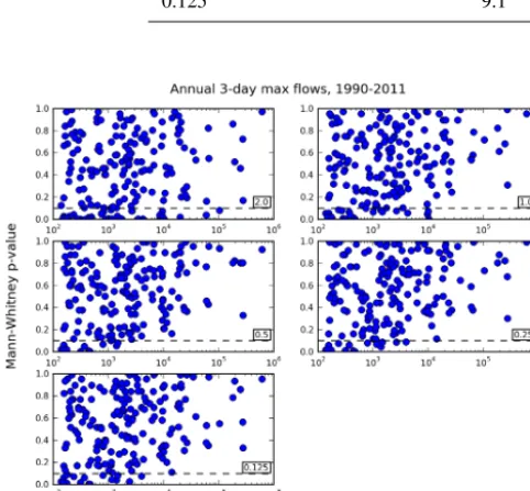
Figure 8.Pvalues from the Mann–WhitneyUtest vs. the drainage area for each of the streamflow sites in Fig. 2. The dashed hori-zontal line at p=0.1 is shown for reference;p values less than this are indicative of poor correspondence between observation- and reanalysis-driven streamflows.
dence between observation- and reanalysis-driven stream-flows is weak. Bias correction at scales smaller than 0.5◦ appears to offer little improvement in skill, and may even result in more streamflow sites having poor skill (p< 0.1). This apparent 0.5◦limit may reflect both the finest scale at which the large-scale reanalysis variance in meteorology can be effectively rescaled (Maraun, 2013) and the degradation of larger-scale spatial structure of driving meteorology (Bár-dossy and Pegram, 2012) when applying quantile-mapping bias correction at finer spatial scales.
Figure 9 shows the relationship between the Mann– Whitneypvalue and the drainage area for each of the stream-flow sites for 7-day minimum stream-flows. Similar to the 3-day peak flows, there is a weak correspondence between the scale at which the bias correction is performed and the skill for basins of different drainage areas. As with 3-day peak flows, bias correction at 0.5◦appears as a point at which finer scale bias correction does not offer any improvement, and may
in-Figure 9. Similar to Fig. 8, but for the 7-day low flows at each
streamflow site.
crease the number of streamflow sites with poor correspon-dence with observation-driven streamflows. Table 1 summa-rizes the results of Figs. 8 and 9, listing the number of stream-flow sites for which skill is low, both forp< 0.1 andp< 0.05. The bias correction being performed at 0.5◦ is revealed as an optimum, confirming the visual interpretations of Figs. 8 and 9.
[image:9.612.312.549.214.412.2]influ-ence of each step in the BCSD process (as shown in Fig. 1) on the biases, though this could be a fruitful avenue for future research.
4 Conclusions
When applying statistical downscaling methods to adapt cli-mate model data for use in regional hydrologic impacts stud-ies, a bias correction step is typically included. A common method for bias correction is quantile mapping, which can be performed in many different ways. One way in which ap-plications of quantile mapping vary is in the spatial scale at which it is applied, which can range from the large scale of climate model output (generally 1 to 4◦ latitude-longitude) down to the finest resolution of observed data. This experi-ment investigated the effect of the spatial scale at which pre-cipitation (and temperature) is bias corrected (as part of a sta-tistical downscaling approach) on the streamflow produced by a hydrologic model.
Similar to many prior studies, as a surrogate for climate model data, this experiment used reanalysis data, which is at a spatial scale of approximately 1.9◦. A gridded obser-vational data set of daily precipitation and temperature was used as the observational baseline, and was aggregated to spatial resolutions of 0.125, 0.25, 0.5, 1.0, and 2.0◦ to be used in the bias correction step of the statistical downscal-ing scheme. The principal finddownscal-ings were that bias correction at the coarsest scale (2.0◦) performed worst, and performing bias correction at scales finer than 0.5◦ produced little ad-ditional benefit, and even degraded the correspondence be-tween observation-driven streamflows and those driven by downscaled meteorology.
This suggests that the primary assumption inherent in quantile-mapping bias correction, namely, that the biases be-tween modeled and observed meteorological variables for a calibration period are relatively stationary in time and can be applied to a projected period, may become less valid at spa-tial resolution finer than approximately 0.5◦. This may indi-cate a shift in the sources of uncertainty causing the biases as spatial resolution changes. Some biases, such as those caused by inadequate topographic representation in the large-scale model, are better described at fine scales and benefit from having bias correction performed at as fine a scale as pos-sible. Other biases, due to incorrect location of climate fea-tures at the larger scale, may be less able to be corrected at very fine spatial scales (e.g., Maraun and Widmann, 2015). For the region and data sources used in this study, the spatial resolution of 0.5◦, or approximately a 50 km scale, appears to provide an optimal balance between these competing effects. The findings of this study caution against the temptation to apply quantile-mapping bias correction at the finest possi-ble scale, even though it provides the closest correspondence to observations for the calibration period. For independent validation periods, these findings suggest that very fine scale
quantile mapping will perform no better, and possibly worse, than coarsening observations to approximately 0.5◦, and
ap-plying bias correction at that scale.
Author contributions. E. P. Maurer designed the experiment and performed the downscaling. D. L. Ficklin conducted hydrologic modeling. W. Wang provided interpretation of results. E. P. Mau-rer prepared the manuscript with contributions from all co-authors.
Acknowledgements. This work was supported by NASA Earth Exchange (NEX, https://nex.nasa.gov/) at NASA Ames Research Center and the Bay Area Environmental Research Institute.
Edited by: A. Bàrdossy
References
Abatzoglou, J. T. and Brown, T. J.: A comparison of statistical downscaling methods suited for wildfire applications, Int. J. Cli-matol., 32, 772–780, doi:10.1002/joc.2312, 2012.
Arnold, J. G., Srinivasan, R., Muttiah, R. S., and Williams, J. R.: Large Area Hydrologic Modeling and Assessment Part I: Model Development, J. Am. Water Resour. As., 34, 73–89, doi:10.1111/j.1752-1688.1998.tb05961.x, 1998.
Bárdossy, A. and Pegram, G.: Multiscale spatial recorrelation of RCM precipitation to produce unbiased climate change scenar-ios over large areas and small, Water Resour. Res., 48, W09502, doi:10.1029/2011wr011524, 2012.
Barnett, T. P., Pierce, D. W., Hidalgo, H. G., Bonfils, C., Santer, B. D., Das, T., Bala, G., Wood, A. W., Nozawa, T., Mirin, A. A., Cayan, D. R., and Dettinger, M. D.: Human-Induced Changes in the Hydrology of the Western United States, Science, 319, 1080– 1083, doi:10.1126/science.1152538, 2008.
Das, T., Maurer, E. P., Pierce, D. W., Dettinger, M. D., and Cayan, D. R.: Increases in flood magnitudes in Cal-ifornia under warming climates, J. Hydrol., 501, 101–110, doi:10.1016/j.jhydrol.2013.07.042, 2013.
Eden, J. M., Widmann, M., Grawe, D., and Rast, S.: Skill, Correc-tion, and Downscaling of GCM-Simulated PrecipitaCorrec-tion, J. Cli-mate, 25, 3970–3984, doi:10.1175/jcli-d-11-00254.1, 2012. Ehret, U., Zehe, E., Wulfmeyer, V., Warrach-Sagi, K., and Liebert,
J.: HESS Opinions “Should we apply bias correction to global and regional climate model data?”, Hydrol. Earth Syst. Sci., 16, 3391–3404, doi:10.5194/hess-16-3391-2012, 2012.
Ficklin, D. L. and Barnhart, B. L.: SWAT hydrologic model parame-ter uncertainty and its implications for hydroclimatic projections in snowmelt-dependent watersheds, J. Hydrol., 519, 2081–2090, doi:10.1016/j.jhydrol.2014.09.082, 2014.
Ficklin, D. L., Stewart, I. T., and Maurer, E. P.: Projections of 21st Century Sierra Nevada Local Hydrologic Flow Compo-nents Using an Ensemble of General Circulation Models1, J. Am. Water Resour. As., 48, 1104–1125, doi:10.1111/j.1752-1688.2012.00675.x, 2012.
in the Upper Colorado River Basin, PLoS ONE, 8, e71297, doi:10.1371/journal.pone.0071297, 2013.
Ficklin, D. L., Barnhart, B. L., Knouft, J. H., Stewart, I. T., Mau-rer, E. P., Letsinger, S. L., and Whittaker, G. W.: Climate change and stream temperature projections in the Columbia River basin: habitat implications of spatial variation in hydrologic drivers, Hydrol. Earth Syst. Sci., 18, 4897–4912, doi:10.5194/hess-18-4897-2014, 2014.
Flato, G., Marotzke, J., Abiodun, B., Braconnot, P., Chou, S. C., Collins, W., Cox, P., Driouech, F., Emori, S., Eyring, V., Forest, C., Gleckler, P., Guilyardi, E., Jakob, C., Kattsov, V., Reason, C., and Rummukainen, M.: Evaluation of Climate Models, in: Cli-mate Change 2013: The Physical Science Basis. Contribution of Working Group I to the Fifth Assessment Report of the Intergov-ernmental Panel on Climate Change, edited by: Stocker, T. F., Qin, D., Plattner, G.-K., Tignor, M., Allen, S. K., Boschung, J., Nauels, A., Xia, Y., Bex, V., and Midgley, P. M., Cambridge Uni-versity Press, Cambridge, United Kingdom and New York, NY, USA, 741–866, 2013.
Gudmundsson, L., Bremnes, J. B., Haugen, J. E., and Engen-Skaugen, T.: Technical Note: Downscaling RCM precipitation to the station scale using statistical transformations – a com-parison of methods, Hydrol. Earth Syst. Sci., 16, 3383–3390, doi:10.5194/hess-16-3383-2012, 2012.
Haan, C. T.: Statistical Methods in Hydrology, second edition, Iowa State Press, Ames, IA, USA, 496 pp., 2002.
Haerter, J. O., Eggert, B., Moseley, C., Piani, C., and Berg, P.: Sta-tistical precipitation bias correction of gridded model data us-ing point measurements, Geophys. Res. Lett., 42, 1919–1929, doi:10.1002/2015gl063188, 2015.
Hawkins, E. and Sutton, R.: The Potential to Narrow Uncertainty in Regional Climate Predictions, B. Am. Meteorol. Soc., 90, 1095– 1107, doi:10.1175/2009BAMS2607.1, 2009.
Hawkins, E. and Sutton, R.: The potential to narrow uncertainty in projections of regional precipitation change, Clim. Dyn., 37, 407–418, doi:10.1007/s00382-010-0810-6, 2011.
Huth, R.: Statistical downscaling of daily temperature in Central Europe, J. Climate, 15, 1731–1742, 2002.
Hwang, S. and Graham, W. D.: Development and comparative evaluation of a stochastic analog method to downscale daily GCM precipitation, Hydrol. Earth Syst. Sci., 17, 4481–4502, doi:10.5194/hess-17-4481-2013, 2013.
Kalnay, E., Kanamitsu, M., Kistler, R., Collins, W., Deaven, D., Gandin, L., Iredell, M., Saha, S., White, G., Woollen, J., Zhu, Y., Leetmaa, A., and Reynolds, B.: The NCEP/NCAR 40-year reanalysis project, B. Am. Meteorol. Soc., 77, 437–472, 1996. Lafon, T., Dadson, S., Buys, G., and Prudhomme, C.: Bias
correction of daily precipitation simulated by a regional cli-mate model: a comparison of methods, Int. J. Climatol., 1–15, doi:10.1002/joc.3518, 2012.
Li, H., Sheffield, J., and Wood, E. F.: Bias correction of monthly precipitation and temperature fields from Intergovern-mental Panel on Climate Change AR4 models using equidis-tant quantile matching, J. Geophys. Res., 115, D10101, doi:10.1029/2009jd012882, 2010.
Li, J., Sharma, A., Johnson, F., and Evans, J.: Evaluating the effect of climate change on areal reduction factors using re-gional climate model projections, J. Hydrol., 528, 419–434, doi:10.1016/j.jhydrol.2015.06.067, 2015.
Livneh, B., Rosenberg, E. A., Lin, C., Nijssen, B., Mishra, V., An-dreadis, K. M., Maurer, E. P., and Lettenmaier, D. P.: A Long-Term Hydrologically Based Dataset of Land Surface Fluxes and States for the Conterminous United States: Update and Exten-sions, J. Climate, 26, 9384–9392, doi:10.1175/jcli-d-12-00508.1, 2013.
Maraun, D.: Nonstationarities of regional climate model biases in European seasonal mean temperature and precipitation sums, Geophys. Res. Lett., 39, L06706, doi:10.1029/2012gl051210, 2012.
Maraun, D.: Bias Correction, Quantile Mapping, and Downscal-ing: Revisiting the Inflation Issue, J. Climate, 26, 2137–2143, doi:10.1175/jcli-d-12-00821.1, 2013.
Maraun, D.: Reply to “Comment on ‘Bias Correction, Quantile Mapping, and Downscaling: Revisiting the Inflation Issue”’, J. Climate, 27, 1821–1825, doi:10.1175/jcli-d-13-00307.1, 2014. Maraun, D. and Widmann, M.: The representation of location by a
regional climate model in complex terrain, Hydrol. Earth Syst. Sci., 19, 3449–3456, doi:10.5194/hess-19-3449-2015, 2015. Maraun, D., Wetterhall, F., Ireson, A. M., Chandler, R. E., Kendon,
E. J., Widmann, M., Brienen, S., Rust, H. W., Sauter, T., The-meßl, M., Venema, V. K. C., Chun, K. P., Goodess, C. M., Jones, R. G., Onof, C., Vrac, M., and Thiele-Eich, I.: Precipi-tation downscaling under climate change: Recent developments to bridge the gap between dynamical models and the end user, Rev. Geophys., 48, RG3003, doi:10.1029/2009rg000314, 2010. Maurer, E. P., O’Donnell, G. M., Lettenmaier, D. P., and Roads, J.
O.: Evaluation of the land surface water budget in NCEP/NCAR and NCEP/DOE reanalyses using an off-line hydrologic model, J. Geophys Res., 106, 17841–17862, 2001.
Maurer, E. P., Brekke, L. D., Pruitt, T., and Duffy, P. B.: Fine-resolution climate change projections enhance regional climate change impact studies, Eos Trans. AGU, 88, 504, doi:10.1029/2007EO470006, 2007.
Maurer, E. P., Brekke, L. D., and Pruitt, T.: Contrasting Lumped and Distributed Hydrology Models for Estimating Climate Change Impacts on California Watersheds1, J. Am. Water Resour. As., 46, 1024–1035, doi:10.1111/j.1752-1688.2010.00473.x, 2010a. Maurer, E. P., Hidalgo, H. G., Das, T., Dettinger, M. D., and Cayan,
D. R.: The utility of daily large-scale climate data in the assess-ment of climate change impacts on daily streamflow in Califor-nia, Hydrol. Earth Syst. Sci., 14, 1125–1138, doi:10.5194/hess-14-1125-2010, 2010b.
Maurer, E. P., Das, T., and Cayan, D. R.: Errors in climate model daily precipitation and temperature output: time invariance and implications for bias correction, Hydrol. Earth Syst. Sci., 17, 2147–2159, doi:10.5194/hess-17-2147-2013, 2013.
Maurer, E. P., Brekke, L., Pruitt, T., Thrasher, B., Long, J., Duffy, P., Dettinger, M., Cayan, D., and Arnold, J.: An enhanced archive facilitating climate impacts and adaptation analysis, B. Am. Me-teorol. Soc., doi:10.1175/bams-d-13-00126.1, 2014.
Meehl, G. A., Covey, C., Delworth, T., Latif, M., McAvaney, B., Mitchell, J. F. B., Stouffer, R. J., and Taylor, K. E.: The WCRP CMIP3 multimodel dataset: A new era in climate change re-search, B. Am. Meteorol. Soc., 88, 1383–1394, 2007.
Mehrotra, R. and Sharma, A.: Correcting for systematic biases in multiple raw GCM variables across a range of timescales, J. Hy-drol., 520, 214–223, doi:10.1016/j.jhydrol.2014.11.037, 2015. Panofsky, H. A. and Brier, G. W.: Some Applications of Statistics
to Meteorology, The Pennsylvania State University, University Park, PA, USA, 224 pp., 1968.
Piani, C., Haerter, J., and Coppola, E.: Statistical bias correction for daily precipitation in regional climate models over Europe, Theor. Appl. Climatol., 99, 187–192, doi:10.1007/s00704-009-0134-9, 2010.
Pierce, D. W., Cayan, D. R., Maurer, E. P., Abatzoglou, J. T., and Hegewisch, K. C.: Improved Bias Correction Techniques for Hy-drological Simulations of Climate Change, J. Hydrometeorology, 16, 2421–2442, doi:10.1175/JHM-D-14-0236.1, 2015.
Reichler, T. and Kim, J.: How Well Do Coupled Models Simu-late Today’s Climate?, B. Am. Meteorol. Soc., 89, 303–311, doi:10.1175/BAMS-89-3-303, 2008.
Schmidli, J., Frei, C., and Vidale, P. L.: Downscaling from GCM precipitation: A benchmark for dynamical and statistical down-scaling, Int. J. Climatol., 26, 679–689, 2006.
Sheffield, J., Barrett, A., Colle, B., Fernando, D. N., Fu, R., Geil, K. L., Hu, Q., Kinter, J., Kumar, S., Langenbrunner, B., Lom-bardo, K., Long, L. N., Maloney, E., Mariotti, A., Meyerson, J. E., Mo, K. C., Neelin, J. D., Nigam, S., Pan, Z., Ren, T., Ruiz-Barradas, A., Serra, Y. L., Seth, A., Thibeault, J. M., Stroeve, J. C., Yang, Z., and Yin, L.: North American Climate in CMIP5 Experiments. Part I: Evaluation of Historical Simulations of Con-tinental and Regional Climatology, J. Climate, 26, 9209–9245, doi:10.1175/jcli-d-12-00592.1, 2013a.
Sheffield, J., Camargo, S. J., Fu, R., Hu, Q., Jiang, X., Johnson, N., Karnauskas, K. B., Kim, S. T., Kinter, J., Kumar, S., Langenbrun-ner, B., Maloney, E., Mariotti, A., Meyerson, J. E., Neelin, J. D., Nigam, S., Pan, Z., Ruiz-Barradas, A., Seager, R., Serra, Y. L., Sun, D.-Z., Wang C., Xie, S.-P., Yu, J.-Y., Zhang, T., and Zhao, M.: North American climate in CMIP5 experiments, Part II: Evaluation of historical simulations of intraseasonal to decadal variability, J. Climate, 26, 9247–9290, doi:10.1175/JCLI-D-12-00593.1, 2013b.
Snover, A. K., Hamlet, A. F., and Lettenmaier, D. P.: Climate-Change Scenarios for Water Planning Studies: Pilot Applications in the Pacific Northwest, B. Am. Meteorol. Soc., 84, 1513–1518, doi:10.1175/BAMS-84-11-1513, 2003.
Taylor, K. E., Stouffer, R. J., and Meehl, G. A.: An Overview of CMIP5 and the experiment design, B. Am. Meteorol. Soc., 93, 485–498, doi:10.1175/BAMS-D-11-00094.1, 2012.
Teutschbein, C. and Seibert, J.: Is bias correction of re-gional climate model (RCM) simulations possible for non-stationary conditions?, Hydrol. Earth Syst. Sci., 17, 5061–5077, doi:10.5194/hess-17-5061-2013, 2013.
Themeßl, M., Gobiet, A., and Leuprecht, A.: Empirical-statistical downscaling and error correction of daily precipitation from regional climate models, Int. J. Climatol., 31, 1530–1544, doi:10.1002/joc.2168, 2011.
Thrasher, B., Maurer, E. P., McKellar, C., and Duffy, P. B.: Techni-cal Note: Bias correcting climate model simulated daily temper-ature extremes with quantile mapping, Hydrol. Earth Syst. Sci., 16, 3309–3314, doi:10.5194/hess-16-3309-2012, 2012. Tian, D., Martinez, C. J., and Graham, W. D.: Seasonal
Predic-tion of Regional Reference EvapotranspiraPredic-tion Based on Climate Forecast System Version 2, J. Hydrometeorol., 15, 1166–1188, doi:10.1175/jhm-d-13-087.1, 2014.
Tryhorn, L. and DeGaetano, A.: A comparison of techniques for downscaling extreme precipitation over the Northeastern United States, Int. J. Climatol., 31, 1975–1989, doi:10.1002/joc.2208, 2011.
Vrac, M., Stein, M., and Hayhoe, K.: Statistical downscaling of pre-cipitation through nonhomogeneous stochastic weather typing, Clim. Res., 34, 169–184, doi:10.3354/cr00696, 2007.
Watterson, I. G., Bathols, J., and Heady, C.: What Influences the Skill of Climate Models over the Continents?, B. Am. Meteorol. Soc., 95, 689–700, doi:10.1175/bams-d-12-00136.1, 2014. Widmann, M. and Bretherton, C. S.: Validation of mesoscale
pre-cipitation in the NCEP reanalysis using a new grid-cell precipi-tation dataset for the Northwestern United States, J. Climate, 13, 1936–1950, 2000.
Wilby, R. L., Hay, L. E., Gutowski, W. J., Arritt, R. W., Takle, E. S., Pan, Z., Leavesley, G. H., and Clark, M. P.: Hydrologi-cal responses to dynamiHydrologi-cally and statistiHydrologi-cally downsHydrologi-caled climate model output, Geophys. Res. Lett., 27, 1199–1202, 2000. WMO: Manual on Low-flow Estimation and Prediction,
Opera-tional Hydrology Report No. 50, World Meteorological Organi-zation, Geneva, Switzerland, 138, 2009.
Wood, A. W., Leung, L. R., Sridhar, V., and Lettenmaier, D. P.: Hy-drologic implications of dynamical and statistical approaches to downscaling climate model outputs, Climatic Change, 62, 189– 216, 2004.
Yuan, X. and Wood, E. F.: Downscaling precipitation or bias-correcting streamflow? Some implications for coupled general circulation model (CGCM)-based ensemble sea-sonal hydrologic forecast, Water Resour. Res., 48, W12519, doi:10.1029/2012WR012256, 2012.