Multi-objective routing aware of mixed IoT traffic for low-cost wireless Backhauls

(1)

R E S E A R C H

Open Access

Multi-objective routing aware of mixed

IoT traffic for low-cost wireless Backhauls

Vinícius N. Medeiros

*

, Bruno Silvestre and Vinicius C. M. Borges

Abstract

The futuristic wireless networks expects to provide adequate support for distinct kind of applications, their diverse requirements, and scenarios for future Internet systems, such as Internet of Things based on multimedia and sensor data, while figuring out low cost solutions to offload the mobile communication core. In this context, Low-cost Wireless Backhauls (LWBs) can be useful, since they are based on cheap WLAN technologies, such as Wireless Mesh Networks that provide capacity for future IoT applications based on mixed traffic. The routing is a fundamental process to provide communication in these multi-hop networks and multi-objective routing optimization algorithms based on Integer Linear Programming (ILP) models have been studied in the literature to address this problem, but there is a lack of solutions for mixed traffic. For this reason, we propose a novel ILP multi-objective approach, called Multi-objective routing Aware of miXed traffIc (MAXI), which employs three weighted objectives to guide the routing in WMNs with different applications and requirements. In addition, we provide a comparative analysis with other relevant approaches of routing using NS-3 to evaluation based on simulation, that takes into account different types and levels of interference (e.g. co-channel interference and external interference) focused on mixed IoT traffic for elderly healthcare scenario. Finally, we demonstrate the effectiveness of the proposed approach to support the requirements of each application through the appropriate combination of objective functions, mainly in dense scenarios with high level of interference.

Keywords: Low-cost wireless Backhauls, Integer linear programming, Multi-objective routing, Mixed and multiple IoT applications, Wireless mesh networks

1 Introduction

Internet of Things (IoT) has emerged as an important technology for smart environments, because it provides a set of operations (sensing, processing, and communi-cation) combined in small devices. It will give rise to a vast number of applications, such as environmental

mon-itoring [1–3], real time applications [4, 5], surveillance

[6], healthcare [7,8], and agriculture [9,10]. These appli-cations will include IoT appliappli-cations based on general sensing data (low sending rates with or without a time restriction) and multimedia applications (video or vir-tual reality with high transmission rate demand mostly

with delivery restriction) [11]. IoT devices are inexpensive

and are being deployed and connected in large numbers and many public places to enable smart environments

*Correspondence:[email protected]

Instituto de Informática (INF) - UFG, Alameda Palmeiras, Quadra D, Câmpus Samambaia, 74690-900 Goiânia, Brazil

based on a mixed of applications. Thus, there is a huge demand for coverage involving these low-power devices, the aggregate throughput demand, and reduce the end-to-end delay.

The next generations of wireless/mobile networks should support a huge increase in the data traffic demand

[12], diversity of performance requirements and

appli-cations (e.g. augmented reality, telemedicine, M2M/IoT, ultra-resolution videos) and to provide high ubiquity

lev-els. Some new technologies [13] are being developing

to achieve the ultra requirements, such as interference cancellation, LTE-U, FoG, Could-RAN, multi-access edge computing, millimeter wave, and massive MIMO. Besides, the futuristics wireless and mobile networks will also be under significant pressure to keep control of CAPEX and

OPEX costs [12, 14, 15], since mobile operators

can-not count transfer the costs top the mobile users’ bills to pay the development and deployment of these new technologies. In this context, the employment of cheap

(2)

approaches is incentived, such as infrastructure and

spec-trum sharing [16] and heterogeneous networks composed

of existing technologies [17,18]. For instance, Wi-Fi and

ZigBee are the most used and cheap wireless technologies

in heterogeneous networks [19].

In developing and big countries, such as Brazil, Mexico, India, and South Africa, there are a lot of poor and dense communities, which really needs low-cost mobile Internet access options, because they are not able to pay for mobile data plans based on LTE or millimeter wave technologies. Low-cost Wireless Backhauls (LWBs) are based on Wi-Fi technologies and can be a method that enables mobile operator to extend their network access infrastructures to these communities, offering affordable mobile data plans. LWBs have made the Internet ubiquitous through some facilities such as the mobility, low-cost, and versa-tility of the equipment that is installed, which previously depended on fixed and network cable points.

Wireless Mesh Networks (WMNs) can be seen as a

LWBs [20], since they are generally built with low-cost

off-the-shelf hardware, such as Wi-Fi standards (IEEE 802.11a, n, b/g). They provide a solution with a wider range (100 meters) and higher transmission rates (300 Mbps in the IEEE 802.11n standard), and can thus provide increased aggregate throughput through the use of multi-ple wireless network interfaces and multi-channel. WMNs are also a multi-hop communication networks, i.e., the information is forwarded (routed) by a mesh router until it reaches the Internet gateway, where it is processed or

stored in the Internet [21, 22]. Moreover, the Wireless

Sensor Networks (WSNs) can be connected to WMNs through the brigde technologies, for instance Raspberry Pi. Thus, WMNs are a promising communication technol-ogy for IoT applications, because they provide a notably high performance and low cost wireless backbone for data in remote locations, when forwarding data from/to the Internet. Hence, WMNs and WSNs can be integrated to allow scenarios with a wide range of IoT applications, in order to reach balance between performance, cost, and ubiquity.

WMNs have a features that directly affect the perfor-mance of these networks, such as multi-hop communi-cation, with a gateway for connection to other wireless or wired networks (by clustering generated data or send-ing data to these networks), as well as interference which restricts the useful capacity of these kinds of networks. In addition, other factors arise as a result of the multi-hop communication carried out by wireless networks, i.e. a) the path size that affects the contention level in the net-work and end-to-end delay (which is important for critical IoT applications) and b) the bottlenecks that are points where nodes are overloaded with traffic and need to be smoothed over to improve the QoS parameters (losses, flow, delay). It should be noted that load balancing, path

length, and interference can be in conflict with each other. For instance, improving load balancing routing leads to an increase in the path length, as well as prevent interfer-ence can impair load balancing and increase path length. In addition, owing to the complex hop-to-hop nature of the communication in these wireless networks, the effec-tiveness of the routing algorithms have a great influence on the quality of the network.

This paper aims to propose an extension of the

multi-objetive routing ILP model in [23], which was carried out

in Wireless Sensor Networks (WSNs), to the routing opti-mization problem in WMNs towards IoT system, with focus on multimedia applications and sensing data from WSNs. The routing problem is based on three objectives: (i) minimize the path length (number of hops), (ii) mini-mize the bottleneck, and (iii) minimini-mize the interference in the path.

The limited transmission speed provided by the IEEE 802.15.4 used in WSNs and the simple traffic application of WSN (i.e. single kind of application) did not enable to

apply the existing model and algorithm in [23] for WMNs

with mixed traffic, since the capacity and constraints char-acteristics of these wireless networks are very different. Therefore we present a reformulation of most objective functions in order to adequate to WMNs based on mixed traffic of future IoT as well as a novel multi-objective routing algorithm. As a result of this, we can take full advantage of WMN characteristics to achieve the overall network performance.

To the best of our knowledge, this is the first work in WMNs that takes into account these three conflict-ing objectives to achieve a more optimized selection of data routes for IoT applications based on mixed traffic. In addition, a comparative analysis is conducted between

two multi-objective routing algorithms [21,22] for

multi-hop wireless networks against the proposed algorithm in this article that are based on ILP (Integer Linear Pro-gramming) mathematical models. In this way it can enable us to analyze important aspects of multi-hop wireless communications in greater depth.

The algorithms were simulated in a multi-channel net-work scenario. Mixed traffic models were used to repre-sent current IoT applications with several requirements, such as video, audio, and sensing data. Moreover this arti-cle also provides the first study of multi-objective routing optimization algorithms based on ILP for multi-hop wire-less networks. Furthermore, it should be emphasized that none of the approaches were previously assessed in a sce-nario with external interference, and thus this study can make a valuable contribution to research by carrying this out here.

This article is structured as follows: In Section 2,

(3)

networks. In Section 3, there will be a description of model multi-objective and present the algorithm MAXI (Multi-objective routing Aware of miXed traffIc for low-cost wireless backhauls) with main features of approach.

In Section 4, we set out the simulation results in

NS-3. The conclusion and suggestions for future work are

summarized in Section5.

2 Related Works

The described studies in this section focus on works that offer solutions that involve the use of multiple objectives to determine the routing.

Boushaba, Hafid, and Gendreau [24] proposed a

source-based routing approach for WMNs, which aims to improve network efficiency by introducing a new metric to determine the link quality, by combining the packet loss rate with interference caused by the inter-flow and intra-flow. This approach seeks to maintain the balance of the gateway by selecting the interface that receives flows on the basis of the average queue size. When two metrics are combined, routes of a good standard can be selected. However, the problem of the bottleneck is critical in the neighborhood of the gateway, when it is not addressed at the intermediate links of the path. Links that are unable to directly bind to the gateway cause secondary bottle-neck points on links with good quality, resulting in packet retransmission and packet loss rate because the device has a full queue.

The study with the title Quality of Experience-based

Routing in Multi-Service Wireless Mesh Networks [25]

employs a QoE-based method of unsupervised reinforced learning to determine the routing in WMNs, and seeks a better experience for the user. The network flows are divided into three types of services (video, audio, and data transfer), and there is a knowledge database of QoS con-straints (delay, packet lost rate, etc.) for each service to determine the routes. At each time interval, this informa-tion is disseminated so that the nodes can update their QoE values through objective calculations. The approach determines individual routes for each type of service with-out taking account of the load balancing in the network.

Zimian Hao and Yingxia Li propose a routing approach

for multi-mesh gateways [26] which includes an

adap-tation of the AODV protocol to disseminate load-aware metrics across the network. The RREQ messages from AODV aims to update the route tables with information about the traffic load on each channel. The RREP mes-sages are used to update the tables with the paths when the destination is found, by determining which links will be used on the route. Although this type of approach seeks to optimize the transmission medium, it creates an over-load of control packets that will reduce the efficiency of the network, as well as controlling the path length needed to reach a certain gateway. In this way, it can both increase

the packet delay and the number of packets delivered, as it adds to contention and bottleneck in the network.

Alwan and Nuha [27] conducted an analysis and

employed a multi-objective optimization method to per-form the WMN routing using Dijkstra’s algorithm and the weighted sum of the objectives (delay and link capac-ity) to determine the WMN routes. The demonstrated method only applies to objectives with linear behavior, and restricts the use of other metrics to determine the routes. The results obtained should be investigated in more realistic environments for a better analysis of the objectives; for example the delay in the delivery of packets might be caused by several situations such as interference, path length, and fairness.

A mathematical formulation for the multi-objective routing problem in hybrid WMN for smart city scenarios

is proposed in [28], where there is a wide range of devices

such as routers, mobile phones, sensors, notebooks, etc. The approach sets out four main factors that must be optimized: path length, delay, packet loss, and energy consumption. In general, energy consumption is not a cru-cial concern in WMN, since in most cases, this kind of network does not have serious energy constraints. The mathematical model is solved through an evolutionary approach, this involves the Strength Pareto Evolutionary Algorithm (SPEA) in a distributed way, since each node is able to calculate its own route (source node) to any other node (target node) by following the mathematical model. All the tests were carried out without the use of a sim-ulator or testbed to validate the definitions specified by the approach. However, this approach is based on some unrealistic assumptions such as the fact that delay is stati-cally defined for each link. Besides, delay and path length are overlapped objectives, since the path length influences significantly the end-to-end delay. In addition, the packet loss rate in a link is determined by means of the distance between the devices that make up the link that is designed to establish the signal strength in the receiver node, which does not depict precisely the link quality. Despite the delay and packet loss are results of regions of load bottlenecks, it is interesting to include an objective function based on load balancing in order to minimize the bottlenecks and thus it can avoid the delay and packet loss before they happen.

Gálvez and Ruiz proposed the routing algorithm called Joint Routing, Channel Assignment and Rate allocation

Heuristic (JRCAR) in [21]. JRCAR determines the

(4)

This approach selects paths that reduce the network bottleneck (load balancing) to enable the algorithm to distribute the flows in a larger number of links. JRCAR defines the bottleneck of any path in WMN as the high-est communication link usage, where the term “usage” is defined as the number of routes that are included in the link. The aim of this study is to balance the instan-taneous traffic in the network through the distribution of the flows, by optimizing the allocation of the channel links to achieve equitable loads in the network. This approach does not take account of the quality of the links and all the tests were carried out with a single type of simple and not very realistic traffic (i.e. only TCP application).

JRCAR generates the routes in the network by means of a pre-established order of flows. The path for each flow is calculated through the number of candidate paths in ascending order. In other words, the routes of the nodes which have fewest alternatives are calculated first. As a result, JRCAR can keep control of its path length, since the most feasible paths have a greater chance of obtaining a path with a similar/equal number of hops while it does not increase the number of bottlenecks.

Mello et al. [22] present a heuristic called Joint approach

for Improving Load balancing and Path length (JILP) for a bi-objective optimization of WMN, where the routes with shortest paths are selected. JILP is responsible for finding solutions for a integer linear multi-objective pro-gramming model that can reduce the number of hops and bottlenecks of the routes in a WMN. This model is able to maintain the lowest bottlenecks in the net-work, and keep control of the routing stability to avoid any unnecessary change of routes. The routing approach is then combined with a channel assignment algorithm to improve network efficiency. However, this approach does not take into account that the scenario is influ-enced by natural physical phenomena, such as inter-ference and signal fading. This may not be enough to provide a good performance, largely because it is sub-ject to signal quality degradation in some regions of the network.

The JILP algorithm is used to add or remove new routes when the flows of the network begin or finish, respectively. If adding a new route leads to an increase in the bottleneck, JILP recalculates the routes involved in the affected links. In a similar way to the JRCAR approach, JILP controls the maximum length of the paths, by means of the same stretch factor as JRCAR, to avoid any degrada-tion of the network performance, although it selects short paths when these include only the flows that pass through the bottleneck. Hence, JILP provides a local routing solu-tion based on traffic demand, which reduces the routing overhead and route fluctuations. However, it can priori-tize the load balancing routing rather than the path length, since it seeks to keep control of the local bottleneck when adding or removing the flow. In addition, it only attempts to reduce the path length for the flows that pass through the bottleneck if it is impossible to obtain the previous smaller value of the bottleneck.

2.1 Comparative Analysis of Related Works

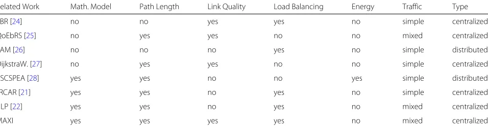
Table1provides a comparison between different routing

approaches of WMNs. This table shows that in the scenar-ios of both WMNs there have been few papers that set out a mathematical model to represent the problem of routing in wireless networks and that use two or more objec-tives to determine the routes. It is important to stress out that none of these approaches addresses the requirements of each application of the mixed traffic when calculat-ing the routes. There are two similar approaches among

those included, JRCAR [21] and JILP [22], that stand out

being the most efficient. This is because they are based on the ILP mathematical model and take into account the main objectives that either directly or indirectly influence the performance parameters (delay, throughput, packet loss rate). However, the used scenarios to evaluate these approaches lack features for current and future applica-tions (such as traffic with different QoS requirements and transmission data rate) and network scenario (such as, a physical layer model that reproduces different levels of interference).

Table 1Related work comparison

Related Work Math. Model Path Length Link Quality Load Balancing Energy Traffic Type

SBR [24] no no yes yes no simple centralized

QoEbRS [25] no yes yes no no mixed centralized

LAM [26] no no no yes no simple distributed

DijkstraW. [27] no yes yes no no simple centralized

RSCSPEA [28] yes yes no no yes simple distributed

JRCAR [21] yes yes no yes no simple centralized

JILP [22] yes yes no yes no mixed centralized

(5)

3 MAXI – Multi-objective routing Aware of miXed traffIc for Low-cost Wireless Backhauls

In this section, we describe the mathematical multi-objective optimization model of ILP (Integer Linear Programming) and an algorithm called MAXI — Multi-objective routing Aware of miXed traffIc to address the single-path routing problem in WMNs. The MAXI algo-rithm employs techniques to simplify the complex task of selecting the set of Pareto optimal solutions.

3.1 Integer Linear Programming Model

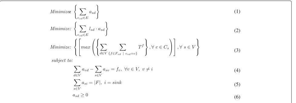
The proposed multi-objective optimization model for the routing in the WMNs is based on three objectives: reduc-ing the number of hops, reducreduc-ing the network bottleneck links, and avoiding the use of low quality links, which significantly affects the application traffic performance of WMNs. These objectives conflict with each other because there is no best solution to achieve all three objectives to an optimal degree. First of all, the number of hops in a required path must be minimized in order to reduce

the end-to-end delay and contention. Figure1shows the

proposed the ILP optimization model.

The interference and contention caused by external and internal sources have a serious impact on the WMN traf-fic performance. However, the physical layer described by the IEEE 802.11 standards can enable the metrics to mea-sure the quality of transmission of a wireless link in a more precise way [29].

One key feature of the future IoT applications is the provision of communication services for the most diverse types of applications, which can allow the transmission and reception of mixed traffic. WMNs must offer var-ied levels of quality of service (QoS) for different types of traffic (data, voice, video), which requires a greater transmission capacity. To achieve this, the objective

function of load balancing must take into account the dif-ferent features of each type of traffic, because applications (e.g. video streaming) with higher transmission rates consume more bandwidth resources in WMNs and for this reason cannot be equated with applications (sensor data) that have considerably lower transmission rates.

It is possible to assign channels between different radios in WMNs that may exist on the devices, and thus improve the data traffic and reduce network contention. The use of multiple channels and multiple radios benefits load bal-ancing between the wireless links since it relieves the total amount of data that make use of the spectrum. Each link has a maximum resource capacity that can be used by the network before it starts causing bottleneck problems, for instance packet loss rate.

WMNs were modeled as a graphG= (V, E), whereV

is the set of vertices that represents the WMN nodes, and

Eis the set of communication links between two network

devices. The link esd ∈ E between the nodess,d ∈ V

can only exist if the devicesaccomplishes a data

trans-mission to the noded. Every node s ∈ V − {i}, where

i is the sink, can be responsible for originating one or

more data streams calledfs ∈ F, whereF is defined as

the set of all the flows generated in the network. All the

flows of the WMNs have the Internet node (sink nodei)

as their destination node. The Internet node is respon-sible for establishing Internet connection with wired networks.

Following this, we will outline the proposed ILP model

(shown in Fig.1), and describe each objective function.

Table2describes the list of variables used in the model.

Number of Hops.A linear programming model is used

to find the shortest paths for f flows in F; the purpose

of the objective function (1) in the model is to find the

minimum number of hops for the solution.

e (1)

(2)

(3)

(4)

(5)

(6)

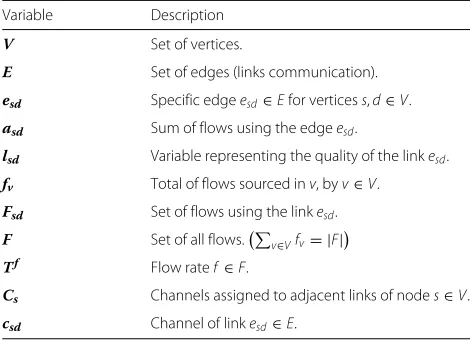
Table 2Description of variables used in system model

Variable Description

V Set of vertices.

E Set of edges (links communication).

esd Specific edgeesd∈Efor verticess,d∈V.

asd Sum of flows using the edgeesd.

lsd Variable representing the quality of the linkesd.

fv Total of flows sourced inv, byv∈V.

Fsd Set of flows using the linkesd.

F Set of all flows._v_∈_Vfv= |F|

Tf _{Flow rate}_f_∈_F_.

Cs Channels assigned to adjacent links of nodes∈V.

csd Channel of linkesd∈E.

Wireless Links with Low QualityThe objective

func-tion (2) uses the l_sd variable to minimize the use of

low-quality links for the paths.

A transmission originating from a node to any other neighbor node is only successful if the Signal to Interfer-ence plus Noise Ratio (SINR) for the receiving node is above a certain threshold. The value of SINR is used as a

basis for obtaining theIR(Interference Ratio) quality

met-ric [24,30] in which the values are represented in a range

from 0 to 1. TheIRis obtained by calculating the relation

between the value of the SINR and the SNR (maximum

tolerable interference level) for the node receptor. TheIR

will be used as a quality metric for the WMNs since it is a more accurate alternative for link quality measurements in

wireless networks. The variation ofIRrepresents an

inter-val from 0 to 1 in which the links can be classified in terms

of their quality. Equation (7) normalizes theIRvalues so

that the link can be classified into low, intermediary and high quality categories.

The variablelsdis responsible for storing the normalized

value of IR, represented by theIRsd variable, which will

indicate the quality of the link between the source node (s)

and the destination node (d) as expressed in Eq. (7). The

lsdvariable is used by the objective function that reduces

the number of low quality links (Eq.2) and must have a

value equal to zero (as defined in Eq. (7-a) so that it can

represent links with a high quality. This is because these links do not add value at the cost of the objective func-tion if the link is used. However, when a link has low or

medium quality (as defined in Eqs. (7-b) and (7-c)) the

value of l_sd must be greater than zero and lower than,

or equal to, 1 (which represents a link with very poor

quality). Hence,IRwas normalized so that the link

qual-ity is classified in a range from 0 (low qualqual-ity) to 1 (high

quality) and moreover, objective function (2) seeks to

min-imize the utilization of links for the path with high values oflsd(one).

An empirical study was carried out to estimate these three link classifications through a set of simulations, i.e. five topologies and six random seeds were generated for each configuration of the number of nodes (10, 20, 30, 40, 50 nodes), resulting in a total of 30 simulations for each

set of node. Table3shows the main configuration

param-eters of scenario of the empirical study, however all the

parameters can be seen in Table6.

lsd=

⎧ ⎪ ⎨ ⎪ ⎩

0, IRsd ≥ Th (a)

1− IRsd−Tl

Th−Tl

, (Th>IRsd >Tl) (b)

1, IRsd ≤ Tl (c)

(7)

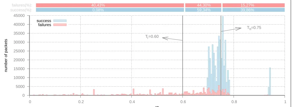
TheTlandThthresholds were fixed so that the the link

quality could be divided in accordance with theIRvalue

that is obtained. Figure2shows the histogram of number

of packet transmissions with failures and successes related

to the Tl andTh thresholds, respectively, as well as the

value ofIR. It is important to note that the packets of this

histogram are only derived from the physical layer taking into account the thresholds of SINR and SNR.

TheTlthreshold was set at 0.60, as there were very few

successful transmissions when the IR was lower than this value; for example, there were 40.43% failed transmissions and 0.08% successful transmissions, so the chances of

suc-cess are low. TheT_hthreshold was set at 0.75, since there

were very few failures in the transmissions when IRwas

higher than, or equal, to 0.75; 15.27% of the transmissions failed and 39.86% of the transmissions were carried out successfully, so the chances of success were high. In light

of this, theTlandThthreshold values were set at 0.60 and

0.75, respectively.

In Fig.2, 44.3% of failures and 59.34% of successes occur

when the value of the IR lies between the limits of Tl

andTh, i.e. there is little difference between success and

failure when links with levels of intermediary quality are used. It is also worth noting that a number of representa-tive success and failure packets are found in this interval.

Equation (7b) assigns the value of thelsd variable in this

interval close to 0 when the IR value approximates to the

value ofT_h, which is the region where the highest

num-ber of successful transmission occurs, and close to 1 when

the IR approximates to the value of Tl, a region where

Table 3Empirical study: NS-3 simulation parameters

Transmission Power 22 (dBm)

Power Detection Threshold -78.0 (dBm)

Carrier Detection Threshold -62.0 (dBm)

Channel Width 20 MHz

Propagation Loss Model Log Distance

Physical layer (NS-3) 802.11n (SpectrumWifiPhy)

(7)

Fig. 2Histogram of successes and failures in transmission as estimated by the IR (link quality metric)

there are no or few attempts that result in a successful transmission.

Network BottleneckOn the one hand, the distribution

of flows in a non-balanced way increases the number of agglomerated flows at the same node (i.e. cause a bottle-neck). This increases the number of forwarded packets and hence leads to delay and adds to the packet loss rate. However, it is possible to employ a set of non-overlapping channels between the different radios presents in the mesh routers through a channel assignment algorithm so that the contention can be mitigated and there can be an improvement in the data traffic performance. Hence,

objective function (3) minimizes the network bottleneck

through a reduction of the largest amount of flow data used by a single channel for all the nodes of network.

ConstraintsThe model imposes three constraints that

can assist in providing a valid solution, i.e. a route in the

network topology. The constraint (4) ensures that every

node (vertex) can only generate a specific numberfv of

flows and the constraint (5) ensures that the Internet

Gateway (i.e. the Internet node) is only able to receive the number of flows generated in the network. This

combi-nation of restrictions (4) and (5) ensures that all the flows

have a path to the Internet node. The constraint (6)

pro-vides non-negative values for the number of flows on the

links inasd(The variableasdis defined as the sum of the

flows that use the edgeesdon their route). Although

con-straints (4), (5), and (6) do not guarantee that there will

not be any loops, the constraint (6) ensures that if there

is a viable solution for creating loops, this will increase the cost of the objective function. As a result, this solu-tion will not be an optimal for minimizasolu-tion problem on the basis of the optimality principle of Dijkstra routing algorithm [31].

3.2 Multi-objective routing Aware of miXed traffIc for

low-cost wireless backhauls (MAXI)

The Multi-objective routing Aware of miXed traffIc (MAXI) is a multi-objective algorithm for solving the routing problem that was modeled in the previous sub-section. The MAXI basically uses an algorithm to determine paths at a lower cost (e.g by using Dijk-stra’s algorithm) in a graph that represents a WMN. The values related to the objective functions, i.e the values associated with edges, are changed depending on which nodes have already been assigned their flow routes.

The MAXI algorithm combines three weighted

objec-tive functions (path length minimization (1),

minimiza-tion of links with low quality (2) and mitigation of network

bottlenecks (3)) at each iteration, to calculate a route for

the new flow. Algorithm 1 employs the weighted sum method to assign the weights for each objective function to meet the requirements of the specific application of that flow in line 4. After this, a minimum cost path is

cre-ated using theMCPathfunction(sender;receiver;GRAPH)

for thefs_{flow (line 5), and the path is incorporated in the}

solution set that will contain all the routes for every flow (as can be observed in line 6).

The procedureupdate_values_edges(wp,wl,wb)defined

in lines 10 to 20, calculates the single objective func-tion by combining the three objectives shown in

subsec-tion3.1, where thewp,wl,wbvariables are weighted path

(8)

channels for a set of nodes that use the same channel are calculated in line 15. After this sum has been

cal-culated for the value of the load variable, it is divided

by the maximum load of the network so that it can be standardized in the interval [0,1]. Finally, the values of the

objectives are combined in the single objective function by using the weights assigned in line 18 of the MAXI Algorithm.

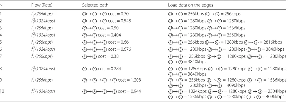
A route is generated for a given flow type at every

iteration algorithm. The Table4shows the stages for

cal-culating the routes represented by Fig.3. Assuming that

the opening sequence of the flows in mesh routers is given

by F = {D,C,A,E,B} and that each mesh router will

generate two types of flows, i.e.f1andf2. The application

that generates f1has a rate of 256kbps and its assigned

weights arewl = 0.6,wp =0.2 andwb=0.2. In contrast,

the application that generatesf2has a rate of 1024kbps

and its assigned weights are as follows:wl = 0.2,wp =

0.2 andw_b=0.6. Given theForder of the devices,

prior-ity is given to every node so that it can generate the routes between the flows originating in that node, as is shown in

the example given in Table4, where initially, the route for

every node is generated for the flow of 256kbpsand soon

afterwards for the flow with a transmission rate equal to

1024kbps.

For each sequence, the Table4shows the data load on

each edge that is used by one or more flows. After adding up all the loads of every flow by means of a specific link, the values are incremented as soon as the new routes have been calculated. The cost variable displays the value of the

path selected for thef_sxstream, wheresis the source node

andxthe type of flow.

The ninth and tenth stages show the difference between

the routing for each flow type: thef_b1flow prefers paths

that have better quality indicators, since they have a greater weight for the quality objective function of the

links (wl). However, a path that distributes the data load

in a balanced way over the network, has been selected

for the f_b2 flow. Thus, distinct paths are selected for

each flow, even though they have the same source node

(i.e. theBnode).

Table 4MAXI Execution sequence

N Flow (Rate) Selected path Load data on the edges

1 f1

d(256kbps) →D →C S cost = 0.70 →D C = 256kbps→C S = 256kbps

2 f2

d(1024kbps) →D →C S cost = 0.548 →D C = 1280kbps→C S = 1280kbps

3 f1

c(256kbps) →C S cost = 0.50 →D C = 1280kbps→C S = 1536kbps

4 f2

c(1024kbps) →C S cost = 0.404 →D C = 1280kbps→C S = 2560kbps

5 f1

a(256kbps) →A →C S cost = 0.66 →A C = 256kbps→D C = 1280kbps→C S = 2816kbps

6 f2

a(1024kbps) →A →C S cost = 0.676 →A C = 1280kbps→D C = 1280kbps→C S = 3840kbps

7 f1

e(256kbps) →E S cost = 0.38 →E S = 256kbps→A C = 1280kbps→D C = 1280kbps

C

→S = 3840kbps

8 f2

e(1024kbps) →E S cost = 0.284 →E S = 1280kbps→A C = 1280kbps→D C = 1280kbps C

→S = 3840kbps

9 f_b1(256kbps) →B →A →C S cost = 1.208 →B A = 256kbps→E S = 1280kbps→A C = 1536kbps

D

→C = 1280kbps→C S = 4096kbps

10 f2

b(1024kbps) →B →A →E S cost = 0.944 →A E = 1024kbps→B A = 1280kbps→E S = 2304kbps A

(9)

Fig. 3Example topology of an WMN

4 Simulation Results

This section presents the comparison of the most rel-evant multi-objective routing algorithms based on ILP model JRCAR, JILP, and MAXI (proposed in the previous section) in the context of future IoT applications based on mixed traffic through a simulation study. The WMNs employed in the performance evaluation should provides key factors to enable an analysis to be conducted of the algorithms:

– The possibility of traffic with high capacity, to support a wide range of applications that may exist in an future IoT context.

– The risk of internal interference, caused by the network nodes themselves, and external interference, caused by devices that are not a part of the network.

For these reasons, we chose an elderly monitoring sys-tem as a suitable example of a set of IoT applications and the NS-3 network simulator to model WMNs that can support the performance requirements of this kind of system as well as to design different levels/types of interference for the wireless network and the applications running on it. This section is structured as follows: there is an outline of the IoT applications and wireless

net-work scenario that is employed in Sub-sections4.1 and

4.2, respectively. The simulation results are discussed in

Sub-section4.3.

4.1 Description of the IoT Applications

WMNs provide a multi-hop wireless infrastructure that enables high-bandwidth traffic to support a wide range of

applications, and allows it to be used in several areas such as scenarios that require higher bandwidth (multimedia applications) or have variable requirements for each appli-cation (for instance, sensors). It should be noted that future IoT applications will combine several applications

with different requirements [32,33]. Owing to the

inher-ent features of future IoT applications, we believe this is a useful application scenario to compare the algorithms studied, since it provides a large number of applications and constraints that can be applied to the infrastructure of a LWB like WMNs.

One example of a future IoT application is the health-care information system where advances in the portable

wireless monitoring system [34] make it more

comfort-able, for example, for an elderly person to be cared for at a nursing home where he/she can be monitored by a portable system. In light of these healthcare applications, there are specific monitoring systems for particular health

problems or preventive monitoring [32, 33]. The cost of

health services and public welfare has been increasing in recent years, especially in countries where people have a high life expectancy. Thus, the challenges to obtain qual-ity services, which meet the needs of elderly people for

example, require these monitoring systems to evolve [35].

(10)

Finally, it is possible to collect information about mobility or falls [32,34–38].

The monitoring devices can be grouped according to

their purpose, location, and monitoring systems [36], for

example:

• Devices for individual use as an accessory (watches, bracelets, necklaces, bandanas).

• Implantable devices (miniaturized video cameras, gastric pressure measurement, continuous glucose monitoring).

• Devices or multimedia systems (video cameras, depth sensor cameras, microphones, smartphones).

• Devices incorporated into clothing.

• Devices adapted to objects, furniture or the floor of the house.

All devices present in a monitoring system for the elderly should have a mean of communicating with the health monitoring center, which manages the care ser-vices and makes it possible to route the data collected by the sensors. Each application, which is built on a set of devices, has different specifications such as data rate

and latency [34, 39]. Thus, the wireless backhaul of the

WMN is a very important to support mixed traffic origi-nating from more than one application using the network to forward the data to a given environment.

In general, the communication architecture for health services can be divided into three categories. The first consists of a network of sensors and devices that is directly linked to the monitored individual. The second level is the WMN which is responsible for sending information from the sensors/devices to the Internet. The third level is the wired network that forward the gathered data by the WMN to the remote monitoring center. Usually, the third level is not necessary if there is a local monitoring center, i.e. it is in the same place that the health services is offered. Thus, all the WSN traffic or that from a spe-cific device (video, microphone, smartphone) is passed through the mesh routers to the medical staff for local

or remote monitoring center [35,40]. We assume a local

monitoring center in this article. The healthcare informa-tion system has several critical requirements that must be taken into account, such as reliable data delivery, privacy,

system response time, etc. [40]. The communication

net-work must provide support to meet these requirements, this means that the links must have enough transfer capac-ity to ensure the generated information can be transmitted and the data is sent using links with good quality to ensure better efficiency.

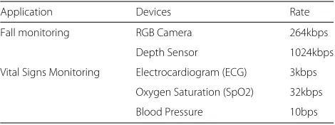
The healthcare system involves a set of devices, each one with specific purpose, constraints, and responsible for generating a flow in the network. In this article, an elderly monitoring is made up of two applications: a

fall monitoring application, generating multimedia flow classes, and a vital sign monitoring application, generating

sensor data flow classes [32,33,36]. Each application flow

has restrictions for these parameters: the fall monitor-ing application uses multimedia traffic and has inherent restrictions of the loss rate, being desirable no more than 20% to 30% losses during data transmission. However, the vital sign monitoring application has delayed packet deliv-ery restrictions, and it is desirable a delay less than 125 ms [34,38].

These two applications can share the same LWB infras-tructure when sending their data. The fall monitoring application can use video devices such as an RGB cam-era, which has a data rate of approximately 264kbps, and

a depth sensor [32], which generates a flow at an

approx-imate rate of 1Mbps. The vital signs monitoring applica-tion uses a set of sensors that perform measurements of a patient’s signals. This set of sensors may vary in accor-dance with the type of monitoring that needs to be carried out; however, most of them are connected to the patient’s

body [34, 35]. In this article, the vital signs monitoring

application employs three types of sensors (each one being responsible for generating a type of flow in the network): electrocardiogram (ECG), with a data rate of 3kbps, oxy-gen saturation (SpO2), with a rate of 32kbps, and blood

pressure sensor, with a rate of 10bps [34,38]. Table5

sum-marizes the applications used to perform the tests and the types of flows that each device generates.

The choice of weights are based on the set of require-ments of the QoS parameters on each application as well as the combination of them in the elderly monitoring system, i.e. loss rate between 20% and 30% for fall mon-itoring application and delay less than 125ms for vital

sign monitoring application [34,38]. In other words, the

requirements and objective functions are associated by giving more and less weight to the objective functions that is somehow influenced and related to the set of applica-tion requirements as well as we set distinct weights for the same objective functions in different applications so that these applications can coexist in the network by taking advantage of the set of alternative routes.

The weights used in the MAXI approach during the

sim-ulations are:wp = 0.50,wl = 0.20,wb = 0.30 for vital

Table 5Summary of the monitoring system for the elderly used in the simulations

Application Devices Rate

Fall monitoring RGB Camera 264kbps

Depth Sensor 1024kbps

Vital Signs Monitoring Electrocardiogram (ECG) 3kbps

Oxygen Saturation (SpO2) 32kbps

(11)

signs monitoring andwp=0.35,wl=0.45 andwb=0.15

for fall monitoring. As the application for vital signs mon-itoring have strong end-to-end delay constraints of the

packets, it was decided to give more weights to thewp

which is referring to the path length. MAXI uses a median

value for the load balancing weightwb= 0.30 in order to

reduce the delay as this helps to reduce waiting time in the queue.

The weights for the fall monitoring application aims to achieve low packet loss rates, so higher values are assigned for the quality goals of the links and path length. The MAXI approach has the weight for the set of links with

low quality (wl = 0.45) and the weight for path length

(wp = 0.35) high, so the selected paths tend to have few

hops and few links with low quality. The fall monitoring has preference in the order of selection of the routes.

4.2 Network Scenario

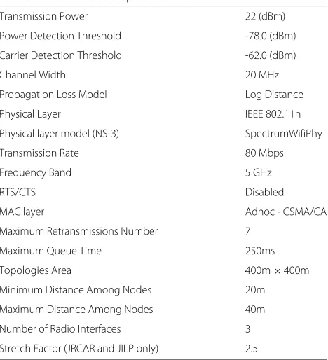
The NS-3 simulator was used in the tests for a better analysis of each algorithm’s performance. NS-3 enables the simulation of a WMN by gathering a more complete

set of the network features. Table 6 shows the general

parameters used in the simulation.

Physical layer model. Physical layer models are mainly

responsible for modeling the reception and transmission of packets and recording energy consumption. The NS-3 simulator provides by default two modules to represent the physical layer of devices for wireless networks:

Yan-sWifiPhy [41] and SpectrumWifiPhy [42].

Table 6NS-3 simulation parameters

Transmission Power 22 (dBm)

Power Detection Threshold -78.0 (dBm)

Carrier Detection Threshold -62.0 (dBm)

Channel Width 20 MHz

Propagation Loss Model Log Distance

Physical Layer IEEE 802.11n

Physical layer model (NS-3) SpectrumWifiPhy

Transmission Rate 80 Mbps

Frequency Band 5 GHz

RTS/CTS Disabled

MAC layer Adhoc - CSMA/CA

Maximum Retransmissions Number 7

Maximum Queue Time 250ms

Topologies Area 400m×400m

Minimum Distance Among Nodes 20m

Maximum Distance Among Nodes 40m

Number of Radio Interfaces 3

Stretch Factor (JRCAR and JILP only) 2.5

The YansWifiPhy model is the standard adopted by NS-3 and is the most widely used model in studies and

implementations, such as in JRCAR [21] and JILP [22], of

Wi-Fi solutions using the NS-3 simulator. Nevertheless, the SpectrumWifiPhy model is an alternative implemen-tation and allows scenarios to be created with the aid several technologies that coexist in the same channel, and thus cause interference among the channels in the same band. In addition, SpectrumWifiPhy provides tools capable of simulating external interference through the

generation of noise [42]. For these reasons, we adopt the

SpectrumWifiPhy model as physical layer model in the simulations.

In this study, the channel assignment algorithm

pro-posed by Gálvez et al. [21] is used which relies on the

distance (in hops) from the devices to the gateway and the quality of the links. This algorithm has been employed in

related works of WMN [21,22].

In this way, the simulations were performed in scenar-ios where the number of nodes ranged from 10 to 50

nodes (Table6) that, on average, represents the number

of devices in the monitoring applications for falls and vital signs. The configuration of traffic loading in the WMNs based on the percentage of mesh routers that actually gen-erate flows, i.e. the percentage of active nodes, which is 100% of active nodes. Each mesh router generates two flows for every IoT device, i.e. 10 flows (two different

applications, displayed in the Table5). Ten topologies and

four random seeds were generated for each configuration of the number of nodes, resulting in a total of 40 simu-lations for each set of nodes. There is a single Internet gateway which is placed in a central position in every topology. The positions of the mesh routers in each topol-ogy were generated through a normal distribution over a limited area, using the topology generation algorithm

from Machado et al. [43]. This ensures that none of the

nodes remain isolated from the network.

4.3 Results Analysis

The results obtained in the simulations will be analyzed using confidence interval based on confidence level of 95% of following performance parameters: throughput, end-to-end delay, path length, and packet loss rate. These parameters are to some extent directly related to each of the objectives that the three approaches (JRCAR, JILP, and MAXI) seek to achieve. This means it will be possible to understand the traffic performance when these routing approaches are taken into account for different numbers of nodes, loads, and interference. The results will be

ana-lyzed in the next sub-sections as follows: Sub-section4.3.1

evaluates the influence of the interference co-channel in

the routing approaches. Sub-section 4.3.2 discusses the

(12)

and routing algorithms for every kind of flow in the healthcare monitoring system.

4.3.1 Co-channel Interference Analysis

The co-channel interference is caused by the activation of the radio on the nodes themselves for data transmis-sion when the same channel or adjacent channels are using

same frequency in a range area [24]. In this context,

sta-tions employ a CSMA/CA protocol and will check if the medium is busy or idle. If the medium is busy, they will defer transmission until it is free. Otherwise, they will attempt to transmit data. Co-channel interference has a negative effect on wireless networks when there is an increase in contention. For instance, as wireless devices attempt to use the spectrum in an area of extreme density, they may have to wait for other devices to complete their transmissions.

Thus, there is a need to evaluate the impact of the co-channel interference on the analyzed algorithms. The SpectrumWifiPhy model simulates the wireless network where it is possible to model interference in a more versatile way. This allows to analyze the impact of the co-channel interference on the network. In this subsec-tion, simulation tests are carried out by using the Spec-trumWifiPhy as a physical layer model varying the number of nodes in the network and making use of 100% of active nodes. This analysis aims to assess the impact of dif-ferent levels of co-channel interference on every routing approach.

Figures 4 and5show the Packet Loss Rate (PLR) and

Average Flow Throughput (AFT) when the number of nodes in the network is increased. It should also be pointed out that MAXI results in the lowest PLR and highest AFT for high density network (i.e. 40 and 50 nodes) with a very high level of contention and interfer-ence. This can be explained by facts that MAXI employs the link quality objective, beyond the two objectives also used in JRCAR and JILP, that minimizes the selection of

Fig. 4PLR - packet loss rate varying the quantity of nodes

Fig. 5Throughput varying the quantity of nodes/load

links with high level of interference as well as giving more weigthed to the load balancing objective function in the vital signs application and link quality objective function in fall monitoring application. JILP and JRCAR achieve similar PLR, since they do not take into consideration the link quality function objective.

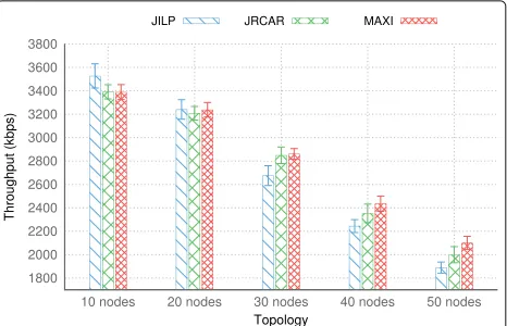
An alternation between JILP and JRCAR can be

observed in throughput (Fig.5). JILP results in a slightly

higher throughput than JRCAR in 10 and 20 nodes, whereas JRCAR achieves the highest throughput in 30, 40, and 50 nodes because it reaches the lowest delay in packet delivery rates and very similar PLR. This can also be explained by the fact that as the number of nodes/load increases, there is also a rise in the contention level. This means that the routing approaches that result in the short-est paths (JRCAR) improve the throughput by reducing contention levels, since they need a lower number of active links to forward the traffic.

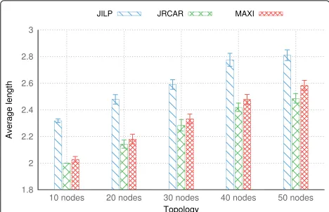
Figure 6 shows the end-to-end delay obtained by the

approaches and Fig.7shows the average path length (in

hops). JRCAR has the lowest average delay, due to the shortest paths achieved by this approach. There are some

(13)

Fig. 7Average path length varying the quantity of nodes

features that explain the delay caused by JRCAR, the stretch factor used in candidate paths and pre-order of flow calculation based on ascending order (i.e. the routes of nodes with the smallest number of alternatives are firstly calculated) and the tie-breaking criteria based on shorter paths when multiple paths have the same values for bottlenecks. As a result of the priorization of load bal-ancing objective, JILP obtains the highest average path length, and therefore, it achieves the highest average delay. MAXI presents an intermediary average delay since it seeks a trade-off among three weighted objectives. There-fore it achieves slightly higher average delay than JRCAR and slightly lower than JILP.

4.3.2 Analyzing the External Interference by varying the number of interferer nodes

Currently, the link quality is the main factor that influ-ences the efficiency of the wireless networks and will continue to do so for some years ahead. Even in the case of IEEE 802.11 standards that still operate in unloaded bands, for instance 5GHz, this issue must be taken into account. This is because the increasing presence of devices with these standards, for instance the IEEE 802.11n and IEEE 802.11ac, will provide greater levels of interference in the future wireless networks that employ these Wi-Fi standards. These devices may have other access points and networks that do not belong to that particular network but by coincidence make use of the same channel. For instance, the LTE-U (LTE-Unlicensed) that proposes the LTE networks use unlicensed spectrum,

mainly in 5Ghz frequency range [18,44]. It is important

to stress out that transmission power of LTE base stations is much higher than Wi-Fi access point and therefore it causes high level of interference. Hence, these examples will certainly occur in extremely dense scenarios which will become increasingly more common in future

net-works [45]. This underlines the importance of analyzing

the results in a scenario where there is a variation of interference levels within the network.

The SpectrumWiFiPhy model makes it possible to include nodes that create electromagnetic waves at certain frequencies, including Wi-Fi, ZigBee, LTE-U, etc., which means these nodes can be used to simulate the interfer-ence caused by devices or even other networks different from WMNs. Simulation tests were carried out to make it easier to assess the impact that the generation of external interference has on the routing approaches, and involved varying the number of nodes that generate external inter-ference from 1 up to 4 nodes. Each node had a power of 0.01 mW and was positioned at the extreme ends of the simulation area so that each interference node is at the same distance to the Internet gateway, as it is shown in

Fig.8. We evaluated the impact of the generated data on

each application listed in Table5.

The power of the interference is modeled by the Power Spectral Density (PSD), and can be defined as the energy distribution per unit of time in a spectrum frequency. In the NS-3 simulation, the PSD is represented by a set of discrete scalar values for each subband of a determined

frequency [42]. This allows the PSD describe how the

power of a signal or times series is distributed over a spec-trum for continuous signals, such as stationary processes

[46]. In this scenario, the interferer node of a spectrum

frequency is other devices (access points) employing IEEE 802.11n or LTE-U. Hence, as the number of interferer nodes increases, there is a rise in the interference level in the network.

(14)

Fig. 9Transmission power - PSD equivalence between a Wi-Fi node and and interference node of the NS-3 interference generator

As it is shown in Fig. 9, an empirical study of

differ-ent transmission power values shows that an interference node of the NS-3 interference generator, when transmit-ting data, using power of 0.01 mW results in a similar PSD of a Wi-Fi node in the IEEE 802.11n (5Ghz)

stan-dard using transmission power about 36 dBm. Table 7

shows the packet delivery rate according to the distance of the receiver node, from 250 meters, the delivery rate decreases a lot (smaller than 40%). It is important to point out that maximum transmission power change accord-ing to country, frequency range, and MCS rate. Under-developed countries such as Lithuania, Indonesia, Thai-land, and South Africa and developed countries such as USA, Canada, China, and Germany usually employ access

points with 36 dBm of maximum transmission power [47].

Many people have acquired in the market Wi-Fi signal amplifiers with low cost or changed the maximum trans-mit power of their routers that can transtrans-mit at maximum power without being aware that they may be causing high levels of interference in other WLAN networks in the area.

Table 7Distance by power reference on NS-3

distance (m) 22dBm 36dBm

40m 100.00% 100.00%

60m 100.00% 100.00%

70m 75.00% 100.00%

71m 70.00% 100.00%

73m 27.50% 100.00%

74m 00.00% 100.00%

220m 0.00% 100.00%

250m 0.00% 84.62%

260m 0.00% 38.46%

262m 0.00% 25.64%

263m 0.00% 0.00%

Given the size of the simulated scenario area, it is pos-sible to assume that there may be a few nodes that use Wi-Fi access points with this transmission power (approx-imately 36 dBm) that can cause considerable interference, especially when considering densely populated areas. For these reasons, a scenario was modeled in this sub-section with some interferer nodes using power of 0.01 mW posi-tioned at the ends to assess traffic performance basing on different routing solutions with different levels of external interference.

Figure10shows the PLR for the three approaches and

all applications. MAXI achieves the lowest PLR in most of the configurations and applications, especially when the number of the interferer node increases. These results can be achieved because MAXI assigns significant weights to

the load balancing objective function (wb = 0.30) in the

vital signs application (Fig.10a, b, and c) and link quality

objective function (wl = 0.45) in fall monitoring

appli-cation (Fig. 10d and e) employs an objective function.

Besides it takes into account of the link quality as objec-tive function. This means that when the links have their quality degraded by the highest number of the interferer nodes, the MAXI approach can find out routes which have a higher link quality, and can thus it achieves a better performance.

JRCAR and JILP fail to take account of the quality of the links in their proposals, which results in a higher packet loss rate. Again, there is an alternation between JILP and JRCAR when varying the number of interferer nodes, JILP reaches lower PLR than JRCAR in one inter-ferer node whereas JRCAR reaches lower PLR for 2, 3, and 4 interferer nodes. Since JILP results in paths with a greater number of hops (as is shown in previous sub-section), this increases the chances of it to use low quality links, that reduce the delivery rate of the data. Basing on this fact, MAXI employs high weights for the path

length objective function in both vital signs (wp = 0.50)

and fall monitoring (wp = 0.35) applications, which also

helps to achieve the lowest PLR for both applications with high level of interference (i.e. 3 and 4 interferer nodes). Although MAXI seeks the equilibrium among number of hops, load balancing, and link quality, it gives preference to the objective functions that can take more advan-tage of specific condition of the scenario to improve the application performance.

Figure11shows the AFT for all applications, where the

MAXI algorithm achieves the highest AFT in most cases of level of interference and applications (especially when the number of the interferer nodes increases). It is worth noting that MAXI keeps the throughput in a very simi-lar value for all levels of interference, whereas JRCAR and JILP diminish the AFT for Blood Pressure, Depth

Sen-sor, and RGB camera video (Fig.11a, d, and e) when the

(15)

0 2 4 6 8 10 12 14 16

1 node 2 nodes 3 nodes 4 nodes

Loss rate (%)

INTERFERER NODES

JILP JRCAR MAXI

10 12 14 16 18 20 22 24 26

Loss rate (%)

INTERFERER NODES

JILP JRCAR MAXI

0 5 10 15 20 25

Loss rate (%)

INTERFERER NODES

JILP JRCAR MAXI

20 22 24 26 28 30 32 34 36

Loss rate (%)

INTERFERER NODES

JILP JRCAR MAXI

20 22 24 26 28 30 32 34

Loss rate (%)

INTERFERER NODES

JILP JRCAR MAXI

(a)

(d) (e)

(b) (c)

Fig. 10Loss rate when varying the number of interferer nodes

increases the AFT in high level of interference (i.e. 3 and

4 interferer nodes) for ECG and RGB camera (Fig.11b

and e) due to fact that link quality objective has the

high-est weigth (wl = 0.45). As JRCAR and JILP do not take

account of the link quality when selecting the routes, the packet loss rate increases which causes a reduction in the throughput, main in JILP.

Figure12(a), (b), and (c) show the average delay obtained

for the flows arising from the vital signs monitoring appli-cations, which needs ultra-low delays due to the urgency of the data delivery, even when there is an increase in the number of interferer nodes. JRCAR results in the low-est delay for most scenarios. However, MAXI results in lower or similar delay compared with JRCAR for some

0.0126 0.0128 0.013 0.0132 0.0134 0.0136 0.0138 0.014 0.0142 0.0144 0.0146 0.0148

Throughput (kbps)

INTERFERER NODES JILP JRCAR MAXI

1 2 3 4 5 6 7 8

Throughput (kbps)

30 32 34 36 38 40 42 44 46

Throughput (kbps)

700 750 800 850 900 950 1000

Throughput (kbps)

220 230 240 250 260 270 280

Throughput (kbps)

(a) (b)

(d) (e)

(c)

(16)

0 5 10 15 20 25

Delay (ms)

0 10 20 30 40 50 60 70 80 90 100

Delay (ms)

0 2 4 6 8 10 12 14

Delay (ms)

150 200 250 300 350 400

Delay (ms)

100 150 200 250 300 350

Delay (ms)

(a)

(d) (e)

(b) (c)

Fig. 12Delay when varying the number of interferer nodes

interference levels and the vital signs monitoring appli-cations, because the path length objective employs the

highest weight for vital signs monitoring (wp= 0.5).

Different levels of interference directly affect the traffic performance, mainly the delay, through the selected route by all routing approaches. As the number of interferer nodes increases, MAXI seeks to determine routes that avoid the use of regions with high levels of interfer-ence. Thus, interference results in a rise in the number of hops, and increases the average end-to-end delay, but not too much when MAXI is employed and moreover, MAXI keeps the delay smaller than the time restriction (125ms). It is important to stress out only the success-ful transmission packets are taken into account for the delay calculation. JRCAR results in higher PLR and lower AFT than MAXI for most interference levels and appli-cations, thus the end-to-end delay can not be too much precise parameter of traffic performance for all routing approaches.

Besides MAXI results in more constant loss rate and throughput when increasing interference and traffic load, the proposal show statistically significant difference,

based on the 2-Sample T test [48], with the second best

approach (JILP or JRCAR) in throughput and loss rate when there are high levels of external interference (i.e. 3 and 4 interferer nodes). In a confidence level of 95%, the 2-Sample T test evidenced a significant difference between the two samples (MAXI and the best second approach (JILP or JRCAR)) for the most network

configu-rations, due the resultantP-value, as it is shown in Table8

whenP-value<0.05, it indicates a significant difference between two samples. In addition, MAXI enables much lesser loss rate (50%, on average of all applications) and higher throughput.

5 Conclusion and Suggestion for Future Works

There is a lacking of routing solutions to support different requirements of mixed traffic for future IoT applications. In this article, we set to cover this gap by introducing a more efficient multi-objetive routing ILP model and algo-rithm, called MAXI, which maximizes the overall mixed traffic performance through supporting the requirements of each application in mixed IoT system. In addition, this article has carried out an in-depth and detailed study of comparison between the main multi-objective routing algorithms for WMNs based on the ILP model, e.g. JRCAR and JILP. The current and future IoT system (monitor-ing for the elderly) with different kinds of applications (camera video RGB, sensor depth, ECG, blood pressure, etc.) and different types of interference (co-channel inter-ference and external interinter-ference) were assessed in a simulated scenario.

(17)

Table 82-Sample T test between MAXI and the second best approach (JILP or JRCAR)

MAXI Second Best Approach

Result Figure Mean Std. Dev. Mean Std. Dev. P-value Approach

PLR Packet Loss Rate 50 node. Figure4 20.88% 4.1777 22.85% 3.7374 0.0291798 JILP

Throughput - (kbps) 50 nodes Figure5 2099.60 176.7813 1999.80 214.1429 0.0258763 JRCAR

PLR Packet Loss Rate 3 interferer nodes Figure10.a 3.88% 3.64508 8.77% 4.3487 6.01526e-7 JRCAR

PLR Packet Loss Rate 4 interferer nodes Figure10.a 4.71% 3.79077 10.87% 4.7405 1.12835e-8 JRCAR

PLR Packet Loss Rate 3 interferer nodes Figure10.b 14.73% 6.0360 20.68% 5.1981 0.000010434 JRCAR

PLR Packet Loss Rate 4 interferer nodes Figure10.b 16.59% 5.8581 21.74% 6.4999 0.000375204 JRCAR

PLR Packet Loss Rate 3 interferer nodes Figure10.c 10.38% 6.3970 15.27% 5.8087 0.0005940690 JILP

PLR Packet Loss Rate 4 interferer nodes Figure10.c 11.39% 6.4491 18.20% 6.2584 0.0771206e-4 JRCAR

PLR Packet Loss Rate 3 interferer nodes Figure10.d 26.11% 6.6300 28.63% 6.0063 0.078334* JRCAR

PLR Packet Loss Rate 4 interferer nodes Figure10.d 25.46% 6.9406 29.58% 6.5963 0.0078889 JRCAR

PLR Packet Loss Rate 3 interferer nodes Figure10.e 24.92% 5.7788 28.29% 7.0203 0.0214786 JILP

PLR Packet Loss Rate 4 interferer nodes Figure10.e 25.46% 6.6399 29.50% 7.0977 0.0103543 JRCAR

Throughput - (kbps) 3 interferer nodes Figure11.a 0.0142 0.0005 0.0129 0.0007 4.73843e-13 JILP

Throughput - (kbps) 4 interferer nodes Figure11.a 0.0141 0.0005 0.0132 0.0007 3.87685e-9 JRCAR

Throughput - (kbps) 3 interferer nodes Figure11.b 5.6153 7.4809 3.8274 3.0998 0.168543* JILP

Throughput - (kbps) 4 interferer nodes Figure11.b 4.2828 1.8386 3.6457 0.2723 0.0360313 JRCAR

Throughput - (kbps) 3 interferer nodes Figure11.c 42.5862 6.0842 37.7976 0.2702 0.00001364 JILP

Throughput - (kbps) 4 interferer nodes Figure11.c 39.6792 3.0428 37.1380 3.0790 0.00038309 JRCAR

Throughput - (kbps) 3 interferer nodes Figure11.d 894.7601 82.7290 903.9110 88.4366 0.634047* JRCAR

Throughput - (kbps) 4 interferer nodes Figure11.d 908.0184 91.2944 900.2777 78.0516 0.684719* JRCAR

Throughput - (kbps) 3 interferer nodes Figure11.e 271.6090 21.8762 258.0036 19.8047 0.0046429 JRCAR

Throughput - (kbps) 4 interferer nodes Figure11.e 268.8379 21.9425 257.3389 26.0504 0.0359653 JRCAR

*_{samples with a}_P-value_≥_0.05

and loss rate are improved significantly when MAXI is employed in network configurations with high levels of external and co-channel interference. In future work, this article will raise an open issue that needs attention, i.e. how to adapt dynamically the weights for mixed IoT

traf-fic based on regular and sporadic data and, theThandTl

thresholds ofIR.

5.1 Source codes

All source codes for the algorithms used in this article

are at the following link::https://github.com/vnmedeiros/

MAXI.

Acknowledgments

This work has been partially supported by the CAPES (Brazil).

Funding

CAPES provided a grant scholarhip during this reseach development. CAPES is a Brazilian government agency awarding scholarship grants to graduate and posgraduate students at universities and research centers.

Availability of data and materials

Not applicable.

Authors’ contributions

VN proposed and developed the work and, carried out the simulation assessment, wrote the article. BS was the co-advisor that help to define the

problem and review the article suggesting a lot of content and corrections to the article. VB was the advisor that defined the initial problem and make many suggestions to improve the research and this article. All authors read and approved the final manuscript.

Competing interests

The authors declare that they have no competing interests.

Publisher’s Note

Springer Nature remains neutral with regard to jurisdictional claims in published maps and institutional affiliations.

Received: 20 November 2018 Accepted: 4 March 2019

References

1. Mainwaring A, Culler D, Polastre J, Szewczyk R, Anderson J. Wireless sensor networks for habitat monitoring. In: Proceedings of the 1st ACM International Workshop on Wireless Sensor Networks and Applications. New York: ACM; 2002. p. 88–97.

2. Cerpa A, Elson J, Estrin D, Girod L, Hamilton M, Zhao J. Habitat monitoring: Application driver for wireless communications technology. ACM SIGCOMM Comput Commun Rev. 2001;31(2 supplement):20–41. 3. Oliveira L, Rodrigues J. Wireless sensor networks: a survey on

environmental monitoring. J Commun. 2011;6(2):143–51. 4. Alanazi A, Elleithy K. Real-time QoS routing protocols in wireless

multimedia sensor networks: Study and analysis. Sensors. 2015;15(9): 22209.https://doi.org/10.3390/s150922209.