R E S E A R C H
Open Access
A nonmonotone hybrid conjugate gradient
method for unconstrained optimization
Wenyu Li and Yueting Yang
**Correspondence:
[email protected] School of Mathematics and Statistics, Beihua University, Jilin Street No. 15, Jilin, China
Abstract
A nonmonotone hybrid conjugate gradient method is proposed, in which the
technique of the nonmonotone Wolfe line search is used. Under mild assumptions,
we prove the global convergence and linear convergence rate of the method.
Numerical experiments are reported.
Keywords:
unconstrained optimization; nonmonotone hybrid conjugate gradient
algorithm; global convergence; linear convergence rate
1 Introduction
Let us take the following unconstrained optimization problem:
min
x∈Rn
f
(
x
),
()
where
f
:
R
n→
R
is continuously differentiable. For solving (), the conjugate gradient
method generates a sequence
{
x
k}
:
x
k+=
x
k+
α
kd
k,
d
= –
g
, and
d
k= –
g
k+
β
kd
k–, where
the stepsize
α
k> is obtained by the line search,
d
kis the search direction,
g
k=
∇
f
(
x
k) isthe gradient of
f
(
x
) at the point
x
k, and
β
kis known as the conjugate gradient parameter.
Different parameters correspond to different conjugate gradient methods. A remarkable
survey of conjugate gradient methods is given by Hager and Zhang [].
Plenty of hybrid conjugate gradient methods were presented in [–] after the first
hy-brid conjugate algorithm was proposed by Touati-Ahmed and Storey []. In [], Lu
et al.
proposed a new hybrid conjugate gradient method (LY) with the conjugate gradient
pa-rameter
β
kLY,
β
kLY=
⎧
⎨
⎩
gkT(gk–dk–)
dTk–(gk–gk–)
,
if
|
–
gkTdk–
gk
| ≤
μ
,
μgk
dTk–gk–λdTk–gk–
,
otherwise,
()
where <
μ
≤
λ––σσ,
σ
<
λ
≤
. Numerical experiments show that the LY method is
effec-tive.
At each iteration, the current function value is defined as follows:
f
l(k)=
max
≤j≤m(k)
f
(
x
k–j),()
where
m
() = ,
≤
m
(
k
)
≤
min
{
m
(
k
– ) + ,
M
}
,
M
is some positive integer. Zhang and
Hager [] proposed another nonmonotone line search technique, they adopted
C
kto
replace the current function
f
k, whereC
k=
ζ
k–Q
k–C
k–+
f
kQ
k,
()
Q
= ,
C
=
f
(
x
),
ζ
k–∈
[, ], and
Q
k=
ζ
k–Q
k–+ .
()
To obtain the global convergence (see [, –]) and implement the algorithms, the line
search in the conjugate gradient is usually chosen by a Wolfe line search; the stepsize
α
ksatisfies the following two inequalities:
f
(
x
k+
α
kd
k)
≤
f
(
x
k) +
ρα
kg
kTd
k,
()
g
(
x
k+
α
kd
k)
Td
k≥
σ
g
kTd
k,
()
where <
ρ
<
σ
< . In particular, a nonmonotone version line search can relax the choice
of the stepsize. Therefore the nonmonotone Wolfe line search requires the stepsize
α
kto
satisfy
f
(
x
k+
α
kd
k)≤
f
l(k)+
ρα
kg
kTd
k()
and (), or
f
(
x
k+
α
kd
k)≤
C
k+
ρα
kg
kTd
k()
and ().
The aim of this paper is to propose a nonmonotone hybrid conjugate gradient method
which combines the nonmonotone line search technique with the LY method. It is based
on the idea that the larger values of the stepsize
α
kmay be accepted by the nonmonotone
algorithmic framework and improve the behavior of the LY method.
The paper is organized as follows. A new nonmonotone hybrid conjugate gradient
al-gorithm is presented and the global convergence of the alal-gorithm is proved in Section .
The line convergence rate of the algorithm is shown in Section . In Section , numerical
results are reported.
2 Nonmonotone hybrid conjugate gradient algorithm and global convergence
Now we present a nonmonotone hybrid conjugate gradient algorithm.
Algorithm
Step
. If
g
k<
, then stop. Otherwise, compute
α
kby () and (), set
x
k+=
x
k+
α
kd
k.
Step
. Compute
β
k+by (), set
d
k+= –
g
k++
β
k+d
k,k
:=
k
+ , and go to Step .
Assumption
We make the following assumptions:
(i) The level set
=
{
x
∈
R
n:
f
(
x
)
≤
f
(
x
)
}
is bounded, where
x
is the initial point.
(ii) The gradient function
g
(
x
) =
∇
f
(
x
)
of the objective function
f
is Lipschitz
continuous in a neighborhood
N
of level set
,
i.e.
there exists a constant
L
≥
such that
g
(
x
) –
g
(
x
¯
)
≤
L
x
–
x
¯
,
for any
x
,
x
¯
∈
N
.
Lemma .
Let the sequence
{
x
k}
be generated by Algorithm
.
Then d
kTg
k<
holds for all
k
≥
.
Proof
From Lemma and Lemma in [], the conclusion holds.
Lemma .
Let Assumption
hold and the sequence
{
x
k}
be obtained by Algorithm
,
α
ksatisfies the nonmonotone Wolfe conditions
()
and
().
Then
α
k≥
σ
–
L
g
kTd
kd
k.
()
Proof
From (), we have
(
g
k+–
g
k)Td
k≥
(
σ
– )
g
Tkd
kand by (ii) of Assumption it implies that
(
g
k+–
g
k)
Td
k≤
α
kL
d
k.
By combining these two inequalities, we obtain
α
k≥
σ
–
L
g
Tk
d
kd
k.
Lemma .
Let the sequence
{
x
k}
be generated by Algorithm
and d
Tkg
k<
hold for all
k
≥
.
Then
f
k≤
C
k.
()
Proof
See Lemma . in [].
Lemma .
Let Assumption
hold
,
and the sequence
{
x
k}
be obtained by Algorithm
,
Then
k≥
Q
k+(
d
kTg
k)d
k< +
∞
.
()
Proof
By () and (), we have
f
k+≤
C
k–
c
(
d
T kg
k)d
k,
()
where
c
=
ρ
( –
σ
)/
L
.
From (), (), and (), we have
C
k+=
ζ
kQ
kC
k+
f
(
x
k+)
Q
k+≤
ζ
kQ
kC
k+
C
k–
c
(dTkgk)
dk
Q
k+≤
C
k–
c
Q
k+(
d
T kg
k)
d
k.
()
Since
f
(
x
) is bounded from below in the level set
and by () for all
k
, we know that
C
kis bounded from below. It follows from () that () holds.
Theorem .
Suppose that Assumptions
hold and the sequence
{
x
k}
is generated by the
Algorithm
.
If
ζ
max< ,
then either g
k=
for some k or
lim
k→∞
inf
g
k= .
()
Proof
We prove by contradiction and assume that there exists a constant
> such that
g
k≥
,
k
= , , , , . . . .
()
By Lemma in [], we have
|
β
k|
LY≤
μgk
dTk–gk–λdkT–gk–
. Then we have
d
k
= (
β
LY)
×
d
k––
g
kTd
k–
g
k≤
(
μgk
dTk–gk–λdTk–gk–
)
d
k–
–
g
kTd
k–
g
k. The rest of the proof
is similar to Theorem and Theorem in [], and we also conclude
(
g
T kd
k)d
k≥
k
.
Furthermore, by
ζ
max< and (), we have
Q
k= +
k– j= j i=ζ
k––i≤
–
ζ
max,
()
then
Q
k+(
g
kTd
k)d
k≥
( –
ζ
max)k
,
which indicates
∞ i=
Q
k+(
g
kTd
k)d
k= +
∞
.
3 Linear convergence rate of algorithm
We analyze the linearly convergence rate of the nonmonotone hybrid conjugate gradient
method under the uniform convex assumption of
f
(
x
). The nonmonotone strong Wolfe
line search is adopted in this section, given by () and
g
(
x
k+
α
kd
k)
Td
k≤
–
σ
g
kTd
k.
()
We suppose that the object function
f
(
x
) is twice continuously differentiable and
uni-formly convex on the level set
. Then the point
x
∗denotes a unique solution of the
problem (); there exists a positive constant
τ
such that
f
(
x
) –
f
x
∗≤
∇
f
(
x
)
x
–
x
∗≤
τ
∇
f
(
x
)
,
for all
x
∈
R
n.
()
The above conclusion () can be found in [].
To analyze the convergence of the nonmonotone line search hybrid conjugate gradient
method, the main difficulty is that the search directions do not usually satisfy the direction
condition:
g
kTd
k≤
–
c
g
k,
()
for some constant
c
> and all
k
≥
. The following lemma has proven that the
direc-tion generated by Algorithm with the strong Wolfe line search () and () in this paper
satisfies the direction condition () by the observation for
g
Tkd
k–.
Lemma .
Suppose that the sequence
{
x
k}
is generated by Algorithm
with the strong
Wolfe line search
()
and
(), <
σ
<
λ+μ
.
Then there exists some constant c
>
such that
the direction condition
()
holds
.
Proof
According to the choice of the conjugate gradient parameter
β
kLY, the result is
dis-cussed by two cases. In the first case,
–
g
T k
d
k–g
k≤
μ
,
i.e.
–
μ
≤
g
T k
d
k–g
k≤
+
μ
,
()
then
β
k=
gTk(gk–dk–)
dT
k–(gk–gk–)
. If
β
k≥
, then, by () and
d
T
k–
g
k–< ,
d
kT–g
k≥
and
g
kT(
g
k–
d
k–)
≥
. Furthermore, we have, by (),
g
kTd
k= –
g
k+
g
Tk
(
g
k–
d
k–)
d
Tk–(
g
k–
g
k–)
g
kTd
k–≤
–
g
k–
σ
g
Tk
(
g
k–
d
k–)
d
kT–(
g
k–
g
k–)
g
Tk–d
k–≤
–
g
k–
σ
g
Tk
(
g
k–
d
k–)
–
d
Tk–g
k–g
kT–d
k–= –
g
k+
σ
g
k–
g
kTd
k–≤
–( –
σ
)
g
k–
σ
( –
μ
)
g
k= –( –
σ μ
)
g
k.
()
If
β
k< , we have, by () and (),
g
kTd
k= –
g
k+
g
Tk
(
g
k–
d
k–)
d
Tk–(
g
k–
g
k–)
g
kTd
k–≤
–
g
k+
σ
g
Tk
(
g
k–
d
k–)
d
Tk–(
g
k–
g
k–)
g
kT–d
k–≤
–
g
k+
σ
g
Tk
(
g
k–
d
k–)
–
d
T k–g
k–g
kT–d
k–≤
–
g
k–
σ
g
k–
g
kTd
k–= –( +
σ
)
g
k+
σ
g
kTd
k–= –( +
σ
)
g
k+
σ
( +
μ
)
g
k= –( –
σ μ
)
g
k.
()
In the second case,
–
g
T kd
k–g
k>
μ
,
()
then
β
k=
μgk
dTk–gk–λdTk–gk–
> . By (), we have
g
kTd
k= –
g
k+
μ
g
kd
Tk–
g
k–
λ
d
Tk–g
k–g
kTd
k–≤
–
g
k–
σ μ
g
k(
σ
–
λ
)
d
Tk–
g
k–g
kT–d
k–= –
–
μσ
λ
–
σ
g
k.
()
From () and (), we obtain (), where
c
=
min
{
–
σ μ
, –
λμσ–σ}
> . The proof is
completed.
Lemma .
Suppose the assumptions of Lemma
.
hold and
,
for all k
,
d
k≤
c
g
k,
()
then there exists a constant c
>
such that
α
k≥
c
,
for all k
.
()
Proof
By Lemma . and Lemma ., we have
α
k≥
σ
–
L
g
kTd
kd
k≥
–
σ
–
L
c
g
kc
g
k≥
c
,
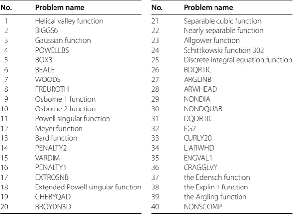
Table 1 Test problems
No. Problem name
1 Helical valley function
2 BIGGS6
3 Gaussian function 4 POWELLBS
5 BOX3
6 BEALE
7 WOODS
8 FREUROTH 9 Osborne 1 function 10 Osborne 2 function 11 Powell singular function 12 Meyer function 13 Bard function 14 PENALTY2
15 VARDIM
16 PENALTY1 17 EXTROSNB
18 Extended Powell singular function
19 CHEBYQAD
20 BROYDN3D
No. Problem name
21 Separable cubic function 22 Nearly separable function 23 Allgower function 24 Schittkowski function 302 25 Discrete integral equation function 26 BDQRTIC 27 ARGLINB 28 ARWHEAD 29 NONDIA 30 NONDQUAR 31 DQDRTIC 32 EG2 33 CURLY20 34 LIARWHD 35 ENGVAL1 36 CRAGGLVY
37 the Edensch function 38 the Explin 1 function 39 the Argling function
40 NONSCOMP
Theorem .
Let x
∗be the unique solution of problem
()
and the sequence
{
x
k}
be
gen-erated by Algorithm
with the nonmonotone Wolfe conditions
()
and
(), <
σ
<
λ+μ
.
If
α
k≤
ν
and
ζ
max< ,
then there exists a constant
ϑ
∈
(, )
such that
f
k–
f
x
∗≤
ϑ
kf
–
f
x
∗.
()
Proof
The proof is similar to that Theorem . given in []. By (), (), and (), we have
f
k+≤
C
k+
ρα
kg
kTd
k≤
C
k–
cc
ρ
g
k.
()
By (ii) in Assumption ,
x
k+=
x
k+
α
kd
kand (), we have
g
k+ ≤g
k+–
g
k+
g
k≤
α
kL
d
k+
g
k≤
( +
c
ν
L
)
g
k.
()
In the first case,
g
k≥
β
(
C
k–
f
(
x
∗)), where
β
= /
cc
ρ
+
τ
( +
c
ν
L
)
.
()
By () and (), we have
C
k+–
f
x
∗=
ζ
kQ
k(
C
k–
f
(
x
∗)) + (
f
k+
–
f
(
x
∗))
+
ζ
kQ
k≤
ζ
kQ
k(C
k–
f
(
x
∗)) + (
C
k–
f
(
x
∗)) –
cc
ρ
g
k +
ζ
kQ
k=
C
k–
f
x
∗–
cc
ρ
g
k
Q
k+.
()
Since
Q
k+≤
–ζmaxby (), we have
C
k+–
f
x
∗≤
C
k–
f
x
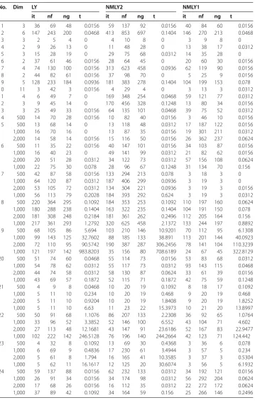
∗Table 2 Numerical comparisons of LY, NMLY1, and NMLY2
No. Dim LY NMLY2 NMLY1
it nf ng t it nf ng t it nf ng t
1 3 36 69 48 0.0156 59 137 92 0.0156 40 84 60 0.0156
2 6 147 243 200 0.0468 413 853 697 0.1404 146 270 213 0.0468
3 3 2 5 4 0 4 10 8 0 3 9 8 0
4 2 9 26 13 0 11 48 28 0 13 38 17 0.0312
5 3 15 28 19 0 29 75 68 0.0312 14 35 28 0
6 2 37 61 46 0.0156 28 64 45 0 20 60 30 0.0156
7 4 74 130 100 0.0156 313 623 458 0.0936 62 119 90 0.0156
8 2 44 82 61 0.0156 37 98 70 0 5 25 9 0.0156
9 5 128 233 184 0.0936 181 383 278 0.1404 104 199 153 0.078
10 11 3 42 3 0.0156 4 29 4 0 3 13 3 0.0312
11 4 6 49 7 0 169 348 254 0.0468 59 121 77 0.0312
12 3 9 45 14 0 170 456 328 0.1248 13 80 34 0.0156
13 3 25 49 33 0.0156 64 135 101 0.0468 39 75 52 0.0312
14 500 14 70 28 0.0156 10 82 40 0.0156 3 46 10 0.0156
15 500 13 68 14 0 13 118 48 0.0312 17 187 122 0.0156
1,000 16 70 16 0 13 87 35 0.0156 19 301 211 0.0312
2,000 14 58 14 0.0156 15 116 50 0.0156 26 362 237 0.0624 16 500 11 35 22 0.0156 40 147 101 0.0156 34 103 87 0.0156
1,000 16 40 23 0 49 141 99 0.0312 21 82 62 0.0156
2,000 20 51 28 0.0312 34 122 73 0.0312 57 156 108 0.0624 1,000 22 75 30 0.078 28 96 67 0.1248 31 134 70 0.156
17 500 42 87 58 0.0156 133 294 213 0.078 3 18 3 0
1,000 64 120 87 0.0312 187 406 299 0.0936 3 19 3 0 2,000 53 105 72 0.0312 134 304 221 0.0936 3 19 3 0.0156 1,000 56 113 79 0.2028 184 393 292 0.624 3 19 3 0.0312 18 500 220 364 295 0.1092 184 353 253 0.1092 110 197 160 0.0624 1,000 180 288 238 0.1404 163 322 235 0.1404 104 191 150 0.078 2,000 181 308 248 0.2184 181 361 262 0.2496 112 205 164 0.156 1,000 217 361 293 1.2792 320 625 458 2.1372 133 244 197 0.8892 19 500 68 105 86 5.694 103 210 146 10.9201 70 112 95 6.1308 1,000 99 143 125 32.7602 88 185 133 38.891 113 201 144 40.0923 2,000 72 110 95 90.5742 190 387 287 306.2456 78 141 104 110.3239 1,000 121 197 142 983.8203 35 156 80 708.6189 24 67 45 322.8129
20 500 51 74 60 0.0468 55 114 73 0.0156 53 83 68 0.0312
1,000 54 78 62 0.0312 55 117 73 0.0312 93 143 115 0.0468 2,000 44 74 58 0.0312 58 130 87 0.0624 33 61 39 0.0156 1,000 43 69 57 0.1872 52 115 71 0.1872 42 75 59 0.1248
21 500 4 9 8 0.0468 10 20 19 0.1092 8 18 17 0.1092
1,000 5 11 10 0.234 10 20 19 0.468 9 20 19 0.468
2,000 5 11 10 0.9204 10 20 19 1.8408 9 20 19 1.8252
1,000 5 11 10 6.63 11 23 22 15.3973 10 21 20 13.8997 22 500 50 91 68 1.1076 86 207 133 2.2308 36 92 65 1.0764 1,000 33 96 52 3.3852 52 146 100 6.552 43 104 71 4.602 2,000 27 113 48 12.1681 43 147 91 23.6186 52 167 83 22.9477 1,000 102 222 142 246.5128 76 196 140 244.2664 42 123 71 124.442
23 500 4 32 8 0.1092 13 69 30 0.4368 3 36 6 0.078
1,000 6 69 9 0.4836 17 230 61 3.4944 3 57 5 0.234
2,000 5 61 8 1.794 16 165 41 10.3585 3 37 3 0.5304
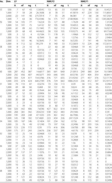
Table 2 (Continued)
No. Dim LY NMLY2 NMLY1
it nf ng t it nf ng t it nf ng t
25 500 7 67 43 12.8545 13 85 53 15.9589 13 80 26 10.4521 1,000 7 59 28 26.7698 8 78 51 41.9019 47 229 130 115.8931 2,000 22 141 90 275.5914 7 55 28 96.081 7 68 28 107.2507 1,000 7 63 36 716.4346 16 175 117 2148.9606 11 115 63 1265.6829 26 500 54 105 77 1.6224 55 127 88 1.7628 46 97 68 1.3728 1,000 53 101 75 5.4132 92 195 140 10.4053 46 94 69 5.0856 2,000 42 89 62 15.1945 71 162 113 27.5654 40 92 65 16.0213 1,000 29 68 43 44.4603 58 150 105 110.0275 44 97 68 69.7168
27 500 3 52 4 0.2184 11 178 91 1.9968 9 152 12 0.6708
1,000 13 193 99 8.7049 5 68 13 1.5756 7 106 27 2.9484 2,000 5 101 46 16.3645 7 141 40 16.5205 7 141 48 18.7045 1,000 9 112 32 99.279 8 140 33 112.5859 13 224 48 172.6151
28 500 8 23 10 0 22 60 38 0.0468 19 45 27 0.0156
1,000 9 25 13 0.0156 7 45 31 0.0156 11 59 43 0.0312
2,000 16 60 26 0.0312 13 78 42 0.0624 16 72 36 0.0468
1,000 5 22 7 0.0312 10 53 30 0.2496 11 60 40 0.2808
29 500 28 65 41 0.0468 13 69 52 0.0312 13 50 27 0.0312
1,000 4 17 5 0 22 86 53 0.0468 11 56 34 0.0156
2,000 7 23 8 0 10 49 26 0.0468 13 66 35 0.0468
1,000 7 26 9 0.0624 4 40 28 0.156 12 124 101 0.7332
30 500 287 452 387 14.6017 365 691 649 21.0913 249 380 334 10.1089 1,000 292 456 407 44.5071 343 646 593 69.3736 257 404 359 40.8411 2,000 343 524 477 154.3786 376 721 655 213.9242 271 457 376 122.1176 1,000 310 474 424 640.2749 376 729 663 1006.2533 236 412 337 512.9157 31 500 70 110 87 0.3276 73 158 113 0.39 58 115 90 0.2964
1,000 49 88 66 0.468 50 131 93 0.624 30 68 45 0.312
2,000 38 69 49 0.7644 64 142 103 1.3416 34 75 49 0.6396 1,000 27 52 32 2.0904 53 128 90 6.1152 34 85 60 4.0248
32 500 6 50 9 0.0156 53 144 89 0.0624 4 60 6 0
1,000 30 88 44 0.0468 18 211 35 0.0468 6 93 7 0.0156
2,000 3 23 6 0.0156 10 107 16 0.0468 4 45 5 0.0156
1,000 5 39 10 0.0936 8 80 17 0.1872 4 55 8 0.0936
33 500 320 442 406 7.6596 427 822 614 11.8405 4 24 7 0.1248 1,000 268 381 342 20.6233 338 652 483 29.1566 4 25 7 0.39 2,000 195 269 248 47.1435 235 461 342 66.7996 4 25 7 1.2792 1,000 145 198 182 137.4681 223 434 326 247.1524 4 25 7 4.5396 34 500 105 187 146 0.1404 101 234 162 0.156 98 191 143 0.1404 1,000 33 76 49 0.1248 73 197 136 0.2496 97 203 156 0.2028 2,000 123 226 172 0.39 173 416 306 0.6708 89 196 141 0.312 1,000 175 311 243 2.6676 236 537 395 4.6176 151 319 239 2.6676
35 500 12 25 14 0.0468 13 35 23 0.078 5 18 5 0.0156
1,000 12 25 14 0.078 11 30 19 0.1248 5 18 5 0.0312
2,000 11 23 13 0.1716 11 34 23 0.2808 5 18 5 0.0624
1,000 10 23 14 0.9984 10 31 22 1.56 5 18 5 0.2808
36 500 37 228 122 0.6864 10 78 17 0.1404 9 34 16 0.078
1,000 17 75 25 0.2652 11 78 20 0.234 9 51 13 0.156
2,000 37 137 57 1.1076 11 101 21 0.5148 15 90 34 0.6864
1,000 16 82 23 2.496 10 82 18 2.1684 15 76 21 2.106
37 500 11 25 16 0.0156 10 33 19 0 3 17 6 0
1,000 12 26 15 0.0156 11 29 19 0.0156 3 17 6 0
2,000 10 22 12 0.0312 10 27 18 0.0312 3 18 6 0.0156
5,000 8 18 10 0.0936 10 27 18 0.156 3 18 6 0.0624
38 500 6 75 50 0.0156 10 123 72 0.0624 8 105 51 0.0312
1,000 4 63 22 0.0156 7 107 43 0.0468 4 56 24 0.0156
2,000 7 121 65 0.0624 13 211 130 0.1248 8 132 68 0.078
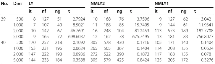
[image:9.595.119.478.122.710.2]Table 2 (Continued)
No. Dim LY NMLY2 NMLY1
it nf ng t it nf ng t it nf ng t
39 500 8 127 51 2.7924 10 168 76 3.7596 9 127 62 3.042
1,000 7 107 40 8.5021 11 188 85 15.7405 9 144 61 11.9341 2,000 10 142 67 46.7691 16 248 104 81.2453 113 573 189 182.7708 5,000 9 165 72 698.6037 12 162 78 675.7495 13 181 83 756.8077 40 500 170 257 218 0.1092 305 578 430 0.1716 105 171 140 0.1404 1,000 153 231 196 0.0624 265 505 367 0.1404 114 208 155 0.0624 2,000 147 222 190 0.0936 272 522 390 0.1872 117 188 155 0.078 5,000 144 233 184 0.3588 305 579 425 0.8424 125 205 172 0.3276
By
g
k≥
β
(
C
k–
f
(
x
∗)), we have
C
k+–
f
x
∗≤
ϑ
C
k–
f
x
∗,
()
where
ϑ
= –
cc
ρβ
( –
ζ
max)∈
(, ).
In the second case,
g
k<
β
(
C
k–
f
(
x
∗)). By () and (), we have
f
k+–
f
x
∗≤
τ
( +
c
ν
L
)
g
k≤
τβ
( +
c
ν
L
)
C
k–
f
x
∗.
By combining the equality, the first equation of (), and
Q
k+≤
–ζmax,
ζ
max< and (),
we obtain
C
k+–
f
x
∗≤
ζ
kQ
k(C
k–
f
(
x
∗)) +
τβ
( +
c
ν
L
)
(
C
k–
f
(
x
∗))
+
ζ
kQ
k=
–
–
τβ
( +
c
ν
L
)
Q
k+C
k–
f
x
∗=
–
–
τβ
( +
c
ν
L
)
( –
ζ
max)C
k–
f
x
∗=
–
cc
ρβ
( –
ζ
max)C
k–
f
x
∗≤
ϑ
C
k–
f
x
∗.
()
By (), (), and (), we have
f
k–
f
x
∗≤
C
k–
f
x
∗≤
ϑ
C
k––
f
x
∗≤ · · · ≤
ϑ
kC
–
f
x
∗.
The proof is completed.
4 Numerical experiments
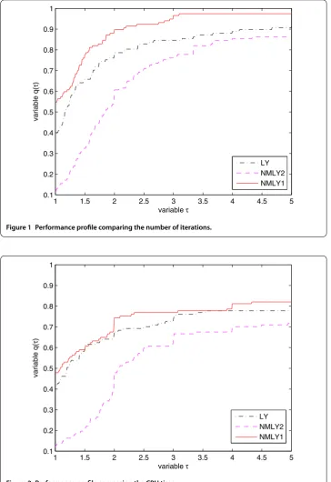
[image:10.595.116.480.97.206.2]Figure 1 Performance profile comparing the number of iterations.
Figure 2 Performance profile comparing the CPU time.
ζ
= .,
ζ
= .,
ζ
k+=
ζk+ζk–, and the terminated condition
g
k
≤
–or
|
f
k+–
f
k| ≤
–max
.,
|
f
k|
.
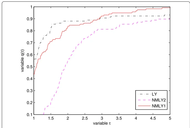
[image:11.595.117.482.83.614.2]Figure 3 Performance profile comparing the number of function evaluations.
Figure 4 Performance profile comparing the number of gradient evaluations.
evaluations. Figure shows the performance of NGLYCG is very much like that of LY
for the number of gradient evaluations. However, the performance of NGLYCG with the
nonmonotone framework () is less than satisfactory.
Competing interests
The authors declare that they have no competing interests.
Authors’ contributions
All authors contributed equally to the writing of this paper. All authors read and approved the final manuscript.
Acknowledgements
This work is supported in part by the NNSF (11171003) of China.
Received: 16 January 2015 Accepted: 27 March 2015
References
1. Hager, WW, Zhang, H: A new conjugate gradient method with guaranteed descent and an efficient line search. SIAM J. Optim.16, 170-192 (2005)
2. Andrei, N: A hybrid conjugate gradient algorithm for unconstrained optimization as a convex combination of Hestenes-Stiefel and Dai-Yuan. Stud. Inform. Control17(4), 55-70 (2008)
3. Babaie-Kafaki, S, Mahdavi-Amiri, N: Two modified hybrid conjugate gradient methods based on a hybrid secant equation. Math. Model. Anal.18(1), 32-52 (2013)
4. Dai, YH, Yuan, Y: An efficient hybrid conjugate gradient method for unconstrained optimization. Ann. Oper. Res.103, 33-47 (2001)
5. Lu, YL, Li, WY, Zhang, CM, Yang, YT: A class new conjugate hybrid gradient method for unconstrained optimization. J. Inf. Comput. Sci.12(5), 1941-1949 (2015)
6. Yang, YT, Cao, MY: The global convergence of a new mixed conjugate gradient method for unconstrained optimization. J. Appl. Math.2012, 93298 (2012)
7. Zheng, XF, Tian, ZY, Song, LW: The global convergence of a mixed conjugate gradient method with the Wolfe line search. Oper. Res. Trans.13(2), 18-24 (2009)
8. Touati-Ahmed, D, Storey, C: Efficient hybrid conjugate gradient techniques. J. Optim. Theory Appl.64(2), 379-397 (1990)
9. Grippo, L, Lampariello, F, Lucidi, S: A nonmonotone line search technique for Newton’s method. SIAM J. Numer. Anal.
23, 707-716 (1986)
10. Zhang, H, Hager, WW: A nonmonotone line search technique and its application to unconstrained optimization. SIAM J. Optim.14, 1043-1056 (2004)
11. Zoutendijk, G: Nonlinear programming, computational methods. In: Abadie, J (ed.) Integer and Nonlinear Programming. North-Holland, Amsterdam (1970)
12. Al-Baali, M: Descent property and global convergence of the Fletcher-Reeves method with inexact line search. IMA J. Numer. Anal.5, 121-124 (1985)
13. Gilbert, JC, Nocedal, J: Global convergence properties of conjugate gradient methods for optimization. SIAM J. Optim.2(1), 21-42 (1992)
14. Yu, GH, Zhao, YL, Wei, ZX: A descent nonlinear conjugate gradient method for large-scale unconstrained optimization. Appl. Math. Comput.187(2), 636-643 (2007)
15. Moré, JJ, Garbow, BS, Hillstrom, KE: Testing unconstrained optimization software. ACM Trans. Math. Softw.7, 17-41 (1981)
16. Andrei, N: An unconstrained optimization test functions collection. Adv. Model. Optim.10, 147-161 (2008) 17. Gould, NIM, Orban, D, Toint, PL: CUTEr and SifDec: a constrained and unconstrained testing environment, revisited.
ACM Trans. Math. Softw.29, 373-394 (2003)