Multiple imputation: an alternative to top coding for statistical disclosure control

©2007 Royal Statistical Society 0964–1998/07/170923

170,Part4,pp.923–940

Multiple imputation: an alternative to top coding for

statistical disclosure control

Di An and Roderick J. A. Little

University of Michigan, Ann Arbor, USA

[Received May 2006. Final revision February 2007]

Summary.Top coding of extreme values of variables like income is a common method of sta-tistical disclosure control, but it creates problems for the data analyst. The paper proposes two alternative methods to top coding for statistical disclosure control that are based on multiple imputation. We show in simulation studies that the multiple-imputation methods provide better inferences of the publicly released data than top coding, using straightforward multiple-impu-tation methods of analysis, while maintaining good statistical disclosure control properties. We illustrate the methods on data from the 1995 Chinese household income project.

Keywords: Confidentiality; Disclosure protection; Multiple imputation

1. Introduction

Statistical disclosure control (SDC) is a class of procedures that deliberately alter data that are collected by statistical agencies before release to the public, to prevent the identity of sur-vey respondents from being revealed. These methods have increased in importance, with the extensive use of computers and the Internet. The goal of SDC methods is to reduce the risk of disclosure to acceptable levels, while releasing a data set that provides as much useful informa-tion as possible for researchers. One aspect of this is the ability to draw valid statistical inferences from the altered data.

Top coding is a simple and common SDC method that seeks to prevent disclosure on the basis of extreme values of a variable, by censoring values above a prechosen ‘top code’. For example, in surveys that include income, extremely high income values are considered to be sensitive and have the potential to reveal the identity of respondents. By recoding income values that are greater than a selected top-code value to that value, respondents with very high income have reduced risk of disclosure.

It is left to the analyst to decide how top-coded data are analysed. One approach is to catego-rize the variable so that top-coded cases all fall in one category—this is sensible but precludes analyses that treat the variable as continuous. Another approach is to ignore the fact of top cod-ing and to treat the top-coded values as the truth. This method is straightforward, but clearly the data distribution is distorted and biased estimates will be obtained. A better method is to treat the extreme values as censored. Under an assumed statistical model, maximum likelihood (ML) estimates can be obtained by using algorithms such as the expectation–maximization (EM) algorithm (Dempsteret al., 1977). This method is model based and should yield good inferences if the model is correctly specified. But we expect this method to be quite sensitive to

Address for correspondence: Roderick J. A. Little, Department of Biostatistics, University of Michigan, 1420 Washington Heights M4045, Ann Arbor, MI 48109-2029, USA.

model misspecification, especially when the upper tail of the assumed distribution differs mark-edly from that of the true distribution. The data users can also apply an imputation method to the top-coded data set and fill in the censored values. A limitation is that the imputed data fail to reflect imputation uncertainty, and imputations are sensitive to assumptions about the right tail of the distribution. We propose alternatives to top coding that allow better inferences for the data user by using simple multiple-imputation (MI) combining rules, while preserving the SDC benefits of top coding.

MI has been proposed as a method of SDC (Little, 1993; Rubin, 1993; Littleet al., 2004; Reiter, 2003, 2005a, b). An imputation model is built from the original data and observed val-ues are replaced by draws from the predictive distribution based on the model. The imputation process is repeated several times and the imputed data sets are then released to the public. Apply-ing this approach to our problem, we delete the data values that are greater than a cut-off point, which is chosen to be smaller than the top code to achieve a mixing of sensitive and non-sensitive values, and apply MI to fill in these values. We then release multiple-imputed data sets to the public. Data users can apply MI combining rules (Reiter, 2003) to obtain valid inferences, as described in Section 3.

We propose non-parametric and parametric MI methods. The non-parametric method is a hot deck procedure, where we replace the deleted values with values that are randomly drawn with replacement from the set of deleted values. The parametric method is Bayesian and assumes a model for the data, draws model parameters from their posterior distribution and then imputes the deleted values with random draws from the posterior predictive distribution.

We compare estimates of the mean of the data from our methods with two estimates from top-coded data. The first, as described previously, is to treat the top-coded values as the true values. The second is to treat those values that are greater than the top code as censored and to apply ML estimation under an assumed model.

We also investigate situations where covariates are present. We use the proposed MI meth-ods to fill in for deleted values without conditioning on covariates. We then perform regression analysis on the imputed data set and compare regression coefficients with those from original and top-coded data. Extensions of our methods that condition on covariate data are also out-lined.

The rest of this paper is organized as follows. Section 2 presents SDC approaches, and Section 3 describes corresponding methods of inference for a population mean. Section 4 describes a simulation study to evaluate the approaches in Section 3, and Section 5 applies the methods to data from the 1995 Chinese household income project. Section 6 considers estimates of regres-sion coefficients for a regresregres-sion where the outcome is subject to our disclosure control methods. Section 7 gives conclusions and discusses future work.

2. Methods of statistical disclosure control

Let Y denote a survey variable (e.g. income) and suppose that values of Y that are greater than a particular valueyTare considered too sensitive for release to the public. We consider the

following approaches to SDC.

(a) Top coding: treatyTas a top-code value, i.e. replace values ofYthat are greater thanyT

byyT. The resulting sample is referred to as ‘top coded’.

(b) Hot deck MI (HDMI): choose a valueyIthat is smaller thanyT. Delete the values of

Y that are greater thanyI and replace them with random draws from the set of deleted

values. We chooseyI< yTto achieve a mixing of sensitive and non-sensitive values. We

(c) Parametric MI (PMI): the HDMI method provides disclosure protection by scrambling sensitive and non-sensitive values, but it is arguably limited from the point of view of SDC, since actual sensitive data values are released. The PMI methods address this concern by releasing data that have been simulated from a parametric model. First, values that are greater than yI are deleted, as with HDMI. The model—we consider the log-normal

model and power-transformed normal model (the power normal model for short)—is fit-ted to the data. Parameters are drawn from their posterior distribution under the assumed model, and deleted values are imputed with draws from their predictive distribution. See Appendix A for details.

Write the complete data asY=.Yret,Ydel/, where Yret denotes the retained values andYdel

denotes the deleted values beyond the cut-off. We consider two versions of PMI, labelled PMIC and PMID. For PMIC, we draw the parameterφof the model for the dataY from its posterior distribution given the complete dataY, i.e.

PMIC :φÅ∼P.φ|Y/:

For PMID, we apply the parametric model to the deleted dataYdeland drawφfrom its posterior

distribution givenYdel:

PMID :φÅ∼P.φ|Ydel/:

The other steps are the same for these two methods, i.e. we draw deleted values from the truncated predictive distribution

Y Å_del∼P.Y|Y > yI,φÅ/:

PMID is less efficient than PMIC since it models the deleted data and fails to exploit fully the information inYwhen drawing values of parameters. However, modelling the deleted data only as in PMID provides useful robustness to model misspecification, as we shall see below.

3. Methods of inference for the mean

We first consider the properties of these SDC methods for inferences about the mean of a variable Ysubject to top coding. Some comments concerning inference for other parameters are provided in Sections 6 and 7. The following estimates and associated standard errors are considered:

(a) before deletion (method BD)—the sample mean of original data.y1,y2, . . . ,yn/before SDC is

ˆ

θ1=1

n n

i=1

yi; .1/

this estimate is used as a bench-mark for comparing SDC methods;

(b) top coding (method TC)—the sample mean of the top-coded data set, namely

ˆ

θ2=1

n n

i=1

yit, .2/

whereyit=yiwhenyi< yTandyit=yTwhenyiyT; this approach is obviously biased,

and our objective is to improve on it with other methods;

The standard errors for methods (a)–(c) are computed by the bootstrap, withB=100 boot-strap samples.

The five remaining methods are all based on MI and createDsets of imputations for values that are beyond the chosen cut pointyI;Dimputed data sets are thus created. For the dth

imputed data setY.d/=.y₁.d/,y₂.d/, . . . ,y.d/_n /, wherey_i.d/=yiifyi< yIandy.d/_i is thedth MI draw

ifyiyI. The MI estimate is then

ˆ

θMI= 1

D D

d=1

ˆ

θ.d/_{, .3/}

where ˆθ.d/is the sample mean of thedth data set. The MI estimate of variance is

TMI=var.θMIˆ /= ¯W+B=D, .4/

whereW¯ =ΣD_d=1W.d/=Dis the average of the within-imputation variancesW.d/for imputed data setd andB=ΣD_d=1.θˆ.d/−θMIˆ /2=.D−1/is the between-imputation variance. Formula (4) dif-fers from the original MI formula for missing data (whereBis multiplied by a factor.D+1/=D; see for example Little and Rubin (2002), page 86), for reasons that were discussed in Reiter (2003). Imputations for these MI methods are created as follows.

(d) Hot deck MI (method HDMI)—imputations are drawn randomly with replacement from the set of values beyond the cut-offyI.

(e) Log-normal MIC (method LNMIC)—imputations are posterior predictions from a log-normal model fitted to the complete data before deletion.

(f) Log-normal MID (method LNMID)—imputations are posterior predictions from a log-normal model fitted to the deleted data beyond the cut-off.

(g) Power normal MIC (method PNMIC)—imputations are posterior predictions from the power normal model, the power-transformed normal distribution fitted to the full data before deletion. For convenience the power transformation is estimated by ML, and parameters are drawn from the full data posterior distribution, treating the power trans-formation as known. An alternative approach is to draw the power from its posterior distribution as well, but we made use of the widely available ML routine box.cox. powers()in R (R Project, 2007) in our calculations.

(h) Power normal MID (method PNMID)—imputations are posterior predictions from the power normal model, fitted to the deleted data beyond the cut-off.

4. Simulation study

A simulation study was carried out to evaluate and compare the SDC methods in Section 3. We computed point estimates of means and the corresponding variances and confidence intervals from the imputed data sets and compared them with those calculated from the original data set before SDC.

4.1. Study design

0

0.00

0.02

0.04

0.06

Den

s

ity 0.0

8

0.10

0.12

0.14

10 20 30

X

40 50 60

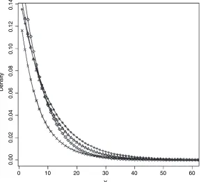
Fig. 1. Tails of the data distributions in the simulation study:, exponential(1);, gamma(1.25, 0.8);

, log-normal(0.2, 0.4);

the usual normal approximation and computed the proportion of CIs that contain the true mean. For parametric estimates in Section 3, the simulated data distributions are allowed to differ from those assumed in the statistical models, to provide an assessment of sensitivity to model misspecification.

In our simulations we chose the 95th percentile of the population distribution as the top-code valueyT. Denote bynSthe number of sensitive sample values that are greater thanyT. We

studied two alternative values for the cut-off pointyI:yI90, the value with 2nSlarger values in

the sample, andyI80, the value with 4nSlarger values in the sample. These values correspond

approximately to the 90th- and 80th-percentile values of the distribution, and for this reason we label the version of a method with an asterisk that uses cut-offyI90‘Å90’ and the version that

uses cut-offyI80‘Å80’.

Clearly the disclosure risk is reduced by increasing the fraction of non-sensitive values that are imputed. A simple measure of the risk of disclosure is the proportion of multiple-imputed values beyond the top-code valueyT. For all the MI methods, this is approximately 50% when

the cut-off point isyI90, and approximately 25% when the cut-off point isyI80.

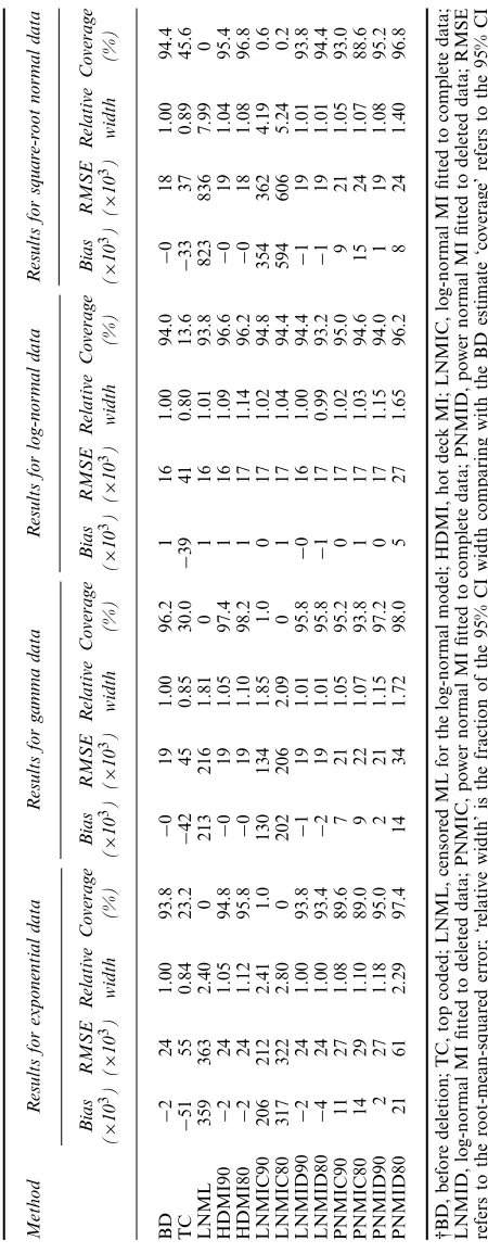
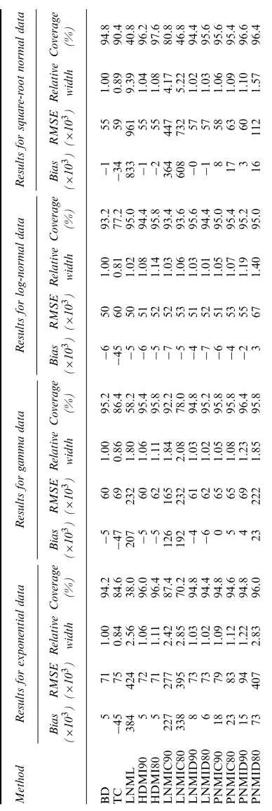
4.2. Results

and HDMI80) have minimal bias and close to nominal coverage for all the simulated popula-tions, with small increases in root-mean-squared error RMSE and CI width compared with the BD estimate. LNML dominates other methods for log-normal data but has serious bias and very poor confidence coverage for the other data sets, suggesting marked sensitivity to model specification. The LNMIC methods have similar properties, although they are less biased and have somewhat better confidence coverage than LNML when the model is misspecified. The LNMID methods are much more robust than their LNMIC counterparts, yielding minimal bias and good confidence coverage for all problems that were simulated.

The PNMIC methods do consistently well in terms of RMSE. Confidence coverage is close to the nominal value, except for exponential data withn=2000 where coverage is a little low. This suggests that the power normal model yields good fits to the range of models that were simulated. The PNMID methods also perform well in terms of bias and confidence coverage, but they are less efficient than the PNMIC methods.

When lowering the cut-off point from yI90 to yI80, we observe minor increases in RMSE

for HDMI, LNMID and PNMIC, and LNMIC when correctly specified. More substantial increases in RMSE are seen for PNMID, and LNMIC when misspecified. The losses in effi-ciency for HDMI80, LNMID80 and PNMIC80 may be acceptable given the increase in disclo-sure protection.

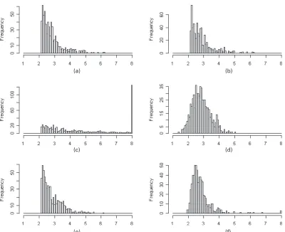
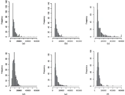
To provide a visual illustration of the imputation methods under potentially misspecified models, Fig. 2 shows the original deleted data values and the imputed values from the HDMI and four PMI methods, with cut-offyI90, for one of the simulated square-root normal data sets

withn=2000. Note that the mean of the deleted values is 2.78. The HDMI predictions look similar to the deleted values and have a similar mean, 2.80.

The LNMIC predictions are too severely skewed and have some extreme predictions, reflect-ing the damagreflect-ing effect on predictions in the tail of applyreflect-ing a misspecified model to the full data set. The LNMIC predictions average 5.68, which is a marked overestimate. In contrast, when the log-normal model is correctly specified, the predictions track the deleted values well (the data are not shown). The LNMID predictions have the shape of a normal distribution, reflect-ing effects of model misspecification, but their mean, 2.72, matches the mean of the deleted values well.

The PNMIC predictions match the deleted values quite well and have a similar mean (2.87), reflecting that this model is correctly specified, since the power normal model includes the square-root normal model as a particular case. The PNMID predictions are more skewed than the deleted values, a reflection that the power normal model does not fit that well when applied to the deleted values; however, these predictions average 2.79, which is very close to the mean of the deleted values.

(a) (b)

(c) (d)

(e) (f)

Fig. 2. Deleted and imputed values for square-root normal data (nD2000) (values greater than 8 are

pooled into one category): (a) deleted values, meanD2:78; (b) imputed (HDMI), meanD2:80; (c) imputed

(LNMIC), meanD5:68; (d) imputed (LNMID), meanD2:72; (e) imputed (PNMIC), meanD2:87; (f) imputed

(PNMID), meanD2:79

5. Application

We applied the above SDC methods to a subset of data from the 1995 Chinese household income project, which was conducted by the Inter-university Consortium for Political and Social Research at the University of Michigan (Riskinet al., 2000). This project was designed to measure the per-sonal income distribution in the People’s Republic of China in 1995. Income information on both households and individuals was recorded for rural and urban areas. Since SDC was not applied to the released data set, the effectiveness of the various SDC methods can be readily assessed.

5.1. Data analysis

Table 3. Comparison of mean estimates, 1995 Chinese household income project, urban and rural data

Method Results for the urban data Results for the rural data

Estimate Fractional Standard Relative Estimate Fractional Standard Relative deviation error of 95% CI deviation error of 95% CI

from BD estimate width from BD estimate width

mean (%) mean (%)

BD 6196 0 36 1.0 2196 0 339 1.0

TC 5895 −4.86 25 0.70 1969 −10.36 25 0.65

LNML 7732 25.8 85 2.38 2675 21.8 59 1.53

HDMI90 6196 −0 41 1.16 2196 0 45 1.16

HDMI80 6196 −0 43 1.19 2197 0.01 47 1.22

LNMIC90 6760 9.10 58 1.61 2512 14.39 70 1.80

LNMIC80 7320 18.14 69 1.92 2653 20.80 77 1.98

LNMID90 6174 −0.35 33 0.92 2179 −0.81 36 0.93

LNMID80 6162 −0.55 32 0.90 2164 −1.46 35 0.90

PNMIC90 6035 −2.60 29 0.80 2205 0.39 39 1.01

PNMIC80 6089 −1.73 30 0.83 2223 1.21 41 1.05

PNMID90 6135 −1.98 37 1.03 2196 −0.02 70 1.80

PNMID80 6108 −1.41 39 1.09 2378 8.26 338 8.74

5.2. Results

Table 3 displays the results from the data analysis. We plot the original deleted data values and the imputed values from the PMI and HDMI methods using cut-off pointyI90in Figs 3 and 4

for the urban and rural data respectively.

Predictably, in both urban and rural cases, method TC underestimates the mean and yields an underestimate of the standard error because of the reduction in standard deviation from top coding. HDMI90 provides the estimate of the mean that is closest to the BD mean, with a 16% increase in standard error. LNML has a large positive bias, indicating sensitivity to the lack of fit of the log-normal model for these data. LNMIC90 is also quite biased, although it performs better than LNML. LNMID90 has negligible bias and a slightly smaller standard error than BD in both the urban and the rural data. The power normal model estimates PNMIC90 and PNMID90 also have small bias. For the urban data, PNMIC90 has relative CI widths that are less than that from BD, which seems anticonservative; for the rural data it has a standard error that is very similar to that of BD. PNMID90 shows a slight increase in CI width for urban data but a large increase in CI width for rural data, reflecting difficulties in fitting this com-plex model to the deleted data. Changing the cut-off point toyI80results in some increases in

bias and standard error for LNMIC80 estimates. Estimates from HDMI80, LNMID80 and PNMIC80 are still acceptable, as are PNMID80 estimates in the urban sample. For the rural data, PNMID80 yields an estimate with strikingly large bias and standard error, the result of some very extreme outliers from imputation. It is important to check that the method is not creating extreme outliers as in this illustration.

6. Study of statistical disclosure control methods with covariates

(a) (b) (c)

(d) (e) (f)

Fig. 3. Deleted and imputed values for the 1995 Chinese household income project, urban data (values

greater than 85 000 are pooled into one category): (a) deleted values, meanD15 164:56; (b) imputed

(HDMI), meanD14 921:94; (c) imputed (LNMIC), meanD20 787:62; (d) imputed (LNMID), meanD14 606:76;

(e) imputed (PNMIC), meanD13 712:23; (f) imputed (PNMID), meanD14 081:03

with those from the original data. Since the MI methods do not condition on the covariates, we expect some bias from this procedure; our interest is in the size of the bias and resulting distortions in confidence coverage.

6.1. Simulation study

Data sets were generated from the following two distributions:

(a) high correlation distribution,

X log.Y/

∼bivariate normal

38 8:6

,

93 5

5 0:38

;

(b) low correlation distribution,

X log.Y/

∼bivariate normal

38 8:6

,

93 2:5 2:5 0:38

:

(a) (b) (c)

(d) (e) (f)

Fig. 4. Deleted and imputed values for the 1995 Chinese household income project, rural data (values

greater than 60 000 are pooled into one category): (a) deleted values, meanD8971:90; (b) imputed (HDMI),

meanD8780:45; (c) imputed (LNMIC), meanD11 777:76; (d) imputed (LNMID), meanD8698:32; (e) imputed

(PNMIC), meanD9103:11; (f) imputed (PNMID), meanD8408:86

their corresponding variances and confidence coverage, as we did for the estimates of the mean in Section 4.

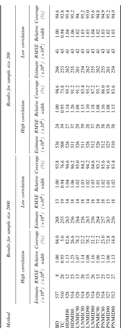
Table 4 displays results for sample sizes 2000 and 200. For data from the high correlation distribution, method TC underestimates the regression coefficient, with large RMSE and very poor confidence coverage. HDMI90 also underestimates the coefficient, as is to be expected since the relationship between the outcome and covariate is attenuated by randomly ‘shuffling’ the values that are beyond the top code. Nevertheless it is less biased and has better coverage than method TC. The other PMI90 methods yield almost the same result as HDMI90. When changing the cut-off point toyI80, all MI methods yield estimates with more bias and RMSE,

reduced efficiency and worse confidence coverage. When the data are from the low correla-tion distribucorrela-tion, all the MI methods have satisfactory properties. This suggests that, for more moderately correlated data, the attenuating effect from imputing without conditioning onX is relatively minor. For the smaller sample size of 200, all the methods are improved in terms of RMSE and coverage, since bias is less of an issue.

individuals and 10 variables, with the logarithm of income treated as the dependent variable. The covariates were age, gender, marital status, level of education, occupation, work environ-ment, work intensity, years of work experience and logarithm of hours worked per week. To simplify the analysis, we investigate only the scenario where the covariates are complete. We applied the top coding, HDMI and PMI methods to the data, where the PMI methods were applied to the marginal distribution of the dependent variable. We again computed estimates of regression coefficients.

We plot standardized regression coefficients after imputation against those from the original data set in Fig. 5. We choose HDMI, LNMID and PNMIC as representations of the MI meth-ods and use the 90th, 80th, 60th and 40th percentiles of the outcome variable as cut-off points, to assess the effect of increasingly severe imputation. We observe that, withyI90, the regression

coefficients from the imputed data set are very close to those from the data set before imputa-tion, and imputation withyI80also has a minor effect on the coefficients. This particular case is

similar to the low correlation scenario from the simulation study. We conclude that, in a situa-tion where the outcome and covariates are not strongly associated, the MI methods proposed are robust to the failure of the imputation model to condition on covariates. Lowering cut-off points results in larger deviation from the original coefficients, leading to greater attenuation of the relationship between outcome and covariates.

7. Discussion

Why should the secondary data analyst prefer our proposed MI methods for SDC to top coding? First, appropriate treatment of the top-coded data, using methods like ML for censored data, requires custom algorithms that are not widely available in standard statistical software; as a result we believe that analysts often treat the top codes as true values and assume that the bias that is introduced by this will be small. In contrast, MI inferences require only complete-data methods and simple MI combining rules. Second, the MI methods tend to be less sensitive than top coding to model misspecification, as seen in our simulation studies. There are two reasons for this—the random draws from the predictive distribution provide variability even if the model is wrong, and the MIs are based on parameter estimates that use information in the original data that is not available in the top-coded data. The data producer is also better able to assess and limit model misspecification, since she or he can compare analyses that are based on the MI data with analyses that are based on the original data. In particular, the imputations from the model can be compared with the true values.

For the data producer, MI has the advantage that the balance between disclosure protection and loss of information can be controlled by the choice of cut-off and number of MIs that are released. The use of MI allows uncertainty of imputation to be propagated, and the MIs of a particular value enhance disclosure protection by making clear to a potential snooper that these values are not real.

(a)

(b)

(c)

(d)

(e)

(f)

(g)

(h)

(i)

(j)

(k)

(l)

Fig.

5.

Standardiz

ed

reg

ression

coefficients,

after

v

ersus

bef

ore

imputation,

1995

Chinese

household

income

project,

urban

data

(

,

y

D

x

):

(a)

HDMI,

cut-off

point

90th

percentile;

(b)

HDMI,

cut-off

point

80th

percentile;

(c)

HDMI,

cut-off

point

60th

percentile;

(d)

HDMI,

cut-off

point

40th

percen

tile;

(e)

LNMID,

cut-off

point

90th

percentile;

(f)

LNMID,

cut-off

point

80th

percentile;

(g)

LNMID,

cut-off

point

60th

percentile;

(h)

LNMID,

cut-off

point

40th

per

centile;

(i)

PNMIC,

cut-off

point

90th

percentile;

(j)

PNMIC,

cut-off

point

80th

percentile;

(k)

PNMIC,

cut-off

point

60th

percentile;

(l)

PNMIC,

cut-off

poi

nt

40th

misspecification, and the PNMID method yielded good confidence coverage but tended to be less efficient than LNMID and PNMIC.

We chose the log-normal and power normal models to illustrate parametric MI, since they are commonly used to model skewed data; they are not universal, and the MI approach could be applied by the data producer with other models that are more suitable for the data at hand. MI that is based on a model fit to all the data (as in the LNMIC and PNMIC meth-ods) is efficient, but vulnerable to model misspecification. Hence, if this approach is adopted, attention to good model specification is needed—in particular, it is important to check that the distribution of the imputed values in the tail is similar to the distribution of the deleted values.

MI that is based on a model fitted to the deleted values alone (the LNMID and PNMID methods) involves some loss of efficiency but is more robust to model misspecification, since the model is being fitted to the data that are being deleted. Here simpler models worked well for the mean, but more refined models may still be needed to get the shape of the distribution in the tail right. We note that, although method TC is generally inferior, it is better than MI when estimating percentiles below the top code but above the cut-off point, since the MI methods delete values in this range that are retained by method TC.

Our results clearly demonstrate the trade-off between reducing the risk of disclosure by allow-ing a larger pool of non-sensitive values for mixallow-ing with the sensitive cases, and reduced efficiency of the estimates. The MI technology is very helpful in propagating the increased uncertainty from the disclosure control method, resulting in good confidence coverage.

MI of deleted values should in principle condition on the observed information, and hence a refinement of the methods proposed is to condition the predictive distribution of the deleted values on observed covariates. Our preliminary assessment of inferences for regression coeffi-cients in Section 6 confirms that a failure to condition on covariates leads to an attenuation of relationships between these covariates and Y. The bias was serious for highly correlated covariates and large samples, but in other situations it was surprisingly minor. This suggests that, when applying the MI method to multivariate data, it may suffice to condition on a rela-tively small set of covariates that are strongly associated with the variable that is subject to SDC. A simple way of doing this for a small set of categorical covariates is to apply the methods that were presented here within strata defined by the covariates, as in the urban and rural strata in the application in Section 5. More generally, regression-based extensions of the methods PNMIC and PNMID can be readily defined by including the key covariates in the mean function. We plan to develop and assess these refinements in future work.

Acknowledgements

This work was supported by National Institute of Child and Human Development grant P01 HD045753. The authors thank Trivellore Raghunathan and three referees for useful comments.

Appendix A: Parametric multiple-imputation method for log-normal model and power-transformed normal model

ForXfrom a log-normal.μ,σ2

/distribution,Y=log.X/∼N.μ,σ2

/. IfXis from the power-transformed normal(μ,σ2_,λ

/distribution withλ=0,Y=.Xλ−1/=λ∼N.μ,σ2

/. To apply the PMI method we estimate λby its ML estimate ˆλby using the widely available routinebox.cox.powers( )in R (see R Project (2007)) and then assume thatY=.Xλˆ−1/=λˆ∼N.μ,σ2

/. (A more principled approach would also simulate λfrom its posterior distribution.)

Given dataY=.y1, . . .yn/from theN.μ,σ2/distribution, the posterior distribution of parameters is

σ2_|

Y∼.n−1/S

2

χ2 n−1

, S2= 1 n−1

n

i=1

.yi− ¯y/2 .5/

and

μ|σ2_,

Y∼N.y¯,σ2

=n/: .6/

We draw parametersμÅandσÅ2_{from their posterior distribution and then draw deleted values for normal} data from the predictive distribution

Y Ådel∼N{μÅ,σÅ

2_|

Y >log.yI/}: .7/

We then transform the draws of normal data back to log-normal,

log-normal:XÅdel=exp.Y Ådel/, .8/

and power-transformed normal data,

XÅdel= ˆ λ √

.λˆY Ådel+1/: .9/

Appendix B: EM algorithm for log-normal model

IfXis log-normal(μ,σ2

/, thenY=log.X/isN.μ,σ2

/andμ=E.X/=exp.μ+σ2

=2/. LetY=.y1, . . . ,yn/ be a random sample fromN.μ,σ2

/, and suppose thatyiis treated as missing if and only ifyi> c, wherec is a known censored value. Without loss of generality, we assume thatyiis observed fori=1, 2, . . . ,rand missing for_i=_r+1, . . . ,_n. The complete-data likelihood is

L.μ,σ|_Y/∝exp

−nlog_.σ_/−n i=1

y2 i 2σ2−

nμ2 2σ2 +μ

n

i=1

yi

σ2

: .10_/

The complete-data sufficient statistics are

S.Y/=

_n

i=1

yi, n

i=1

y2i

: .11/

We write_Y=_.Yobs,Ydel/, whereYobsdenotes the observed values andYmisdenotes the missing values. Given parameter estimatesθ.t/_=.μ.t/_,σ.t/_{/, the (t+1)th iteration of the EM method is as follows:}

(a) E-step,

s.t0+1/=E _n

i=1

yi|Yobs,θ.t/

=r i=1

yi+ n

i=r+1

E.yi|yi> c,θ.t// .12/

=r i=1

yi+.n−r/ ∞

c

y√ 1

.2πσ.t/2_/exp ₋

.y−μ.t/_/2 2σ.t/2

dy

∞

c 1 √

.2πσ.t/2

/exp

₋

.y−μ.t/_/2 2σ.t/2

dy

s.t1+1/=E _n

i=1

y2i|Yobs,θ.t/

=r i=1

y2i+.n−r/ _∞

c

y2√ 1 .2πσ.t/2

/exp

−.y−μ.t/_/2 2σ.t/2

dy

_∞

c 1 √

.2πσ.t/2

/exp

−.y−μ.t/_/2 2σ.t/2

dy

−1

;

.13/

(b) M-step,

μ.t+1/₌

s.t0+1/=n,

σ.t+1/2₌

s.t1+1/=n−s.t+

1/2

0 =n

2

:

.14/

Once the sequence ofθ.t/_{has converged to a stable value (μ˜,σ˜/, we calculate the ML estimate ofμas}

ˆ

θ4= ˜μ=exp.μ˜+ ˜σ2=2/: .15/

References

Dempster, A. P., Laird, N. M. and Rubin, D. B. (1977) Maximum likelihood from incomplete data via the EM algorithm (with discussion).J. R. Statist. Soc.B,39, 1–38.

Fuller, W. A. (1993) Masking procedures for microdata disclosure limitation.J. Off. Statist.,2, 383–406. Little, R. J. A. (1993) Statistical analysis of masked data.J. Off. Statist.,9, 407–426.

Little, R. J., Liu, F. and Raghunathan, T. (2004) Statistical disclosure techniques based on multiple imputation. InApplied Bayesian Modeling and Causal Inference from Incomplete-data Perspectives(eds A. Gelman and X.-L. Meng), pp. 141–152. New York: Wiley.

Little, R. J. A. and Rubin, D. B. (2002)Statistical Analysis with Missing Data. New York: Wiley.

Reiter, J. P. (2003) Inference for partially synthetic, public use microdata sets.Surv. Methodol.,29, 181–188. Reiter, J. P. (2005a) Releasing multiply imputed, synthetic public use microdata: an illustration and empirical

study.J. R. Statist. Soc.A,168, 185–205.

Reiter, J. P. (2005b) Significance tests for multi-component estimands from multiply-imputed, synthetic microdata. J. Statist. Planng Inf.,131, 365–377.

Riskin, C., Zhao, R. and Li, S. (2000) Chinese Household Income Project, 1995. Political Economy Research Institute, University of Massachusetts, Amherst. (Available fromhttp://webapp.icpsr.umich.edu/ cocoon/ICPSR-STUDY/03012.xml.)

R Project (2007)The R Project for Statistical Computing. (Seehttp://www.r-project.org/.)