R E S E A R C H
Open Access
An optimized finite element extrapolating
method for 2D viscoelastic wave equation
Hong Xia
1and Zhendong Luo
2**Correspondence: [email protected] 2School of Mathematics and
Physics, North China Electric Power University, No. 2, Bei Nong Road, Changping District, Beijing, 102206, China
Full list of author information is available at the end of the article
Abstract
In this study, we first present a classical finite element (FE) method for a
two-dimensional (2D) viscoelastic wave equation and analyze the existence, stability, and convergence of the FE solutions. Then we establish an optimized FE
extrapolating (OFEE) method based on a proper orthogonal decomposition (POD) method for the 2D viscoelastic wave equation and analyze the existence, stability, and convergence of the OFEE solutions and furnish the implement procedure of the OFEE method. Finally, we furnish a numerical example to verify that the numerical
computing results correspond with the theoretical ones. This signifies that the OFEE method is feasible and efficient for solving the 2D viscoelastic wave equation.
MSC: 65N15; 65N30
Keywords: classical finite element method; optimized finite element extrapolating method; proper orthogonal decomposition method; error estimate
1 Introduction
Let⊂R be a bounded convex polygonal domain with a smooth boundary∂. We consider the following initial-boundary value problem:
Problem Seekusatisfying
⎧ ⎪ ⎪ ⎨ ⎪ ⎪ ⎩
utt–εut–γ u=f, (x,y,t)∈×(,T],
u(x,y,t) =ϕ(x,y,t), (x,y,t)∈∂×(,T],
u(x,y, ) =ϕ(x,y), ut(x,y, ) =ϕ(x,y), (x,y)∈,
()
whereutt=∂u/∂t,ut=∂u/∂t, andεandγ are two positive constants,f(x,y,t),ϕ(x,y,t), andϕ(x,y) andϕ(x,y) are, respectively, the source term, the boundary value function, and the initial value functions, sufficiently smooth to ensure the validity of the following analysis, andTis the time duration. As a matter of convenience, we assume thatϕ(x,y,t) = andε=γ = in the remaining part of the article.
[–]), because the viscoelastic wave equation in the real-world engineering applications usually has complex known data or computed domains, the analytical solution cannot be generally solved, so one has to find its solutions numerically. For more than years, it has been attentively studied and many numerical methods for the viscoelastic wave equation have been developed (see,e.g., [–]). Among all numerical methods, the finite element (FE) method is considered to be one of the calculating numerical methods with the best theory for the two-dimensional (D) viscoelastic wave equation (see [, ]). Nevertheless, the classical FE methods for the D viscoelastic wave equation are some macroscale sys-tems of equations including lots of unknowns,i.e., degrees of freedom, so entail very large computational load in real-world engineering applications. As a consequence, an impor-tant issue is how to greatly lessen the number of unknowns of the classical FE methods to reduce the computational load, ease the truncated error amassing, and save CPU time in the numerical computation, while preserving the desired FE solution accuracy.
It has been proved by lots of numerical studies (see,e.g., [–]) that the proper or-thogonal decomposition (POD) method is a very useful tool to reduce the number of un-knowns for numerical models and ease the truncated error amassing in numerical calcu-lations. But most existing reduced-order models, as mentioned, were established via the POD basis formed from the classical numerical solutions at all time nodes, before repet-itively computing the reduced-order numerical solutions at the same time nodes, which were some valueless repetitive calculations. Since , some reduced-order FE extrap-olating methods based on the POD method for partial differential equations have been established successively by Luo’s team (see,e.g., [–]) in order to avert the valueless repeated computations.
However, as far as we know, there has not been any report that the POD method is used to reduce the number of unknowns in the classical FE method for the D viscoelastic wave equation. Therefore, in this article, we devote ourselves to building an optimized FE extrapolating (OFEE) method that includes very few unknowns but maintains desired accuracy via the POD method, analyzing the existence, stability, and convergence of the OFEE solutions and verifying the efficiency and feasibility of the OFEE method by some numerical simulations.
for-mulate the POD basis and build the OFEE format so that it does not have repetitive cal-culations, such as done in references [–]. Consequently, it is a development and an improvement of the existing aforementioned ones (see,e.g., [–]).
The remaining content of the article is organized as follows. In Section , we first present the classical FE method for the D viscoelastic wave equation and analyze the existence, stability, and convergence of the classical FE solutions. In Section , we develop the OFEE method via the POD method for the D viscoelastic wave equation, analyze the stability and convergence of the OFEE solutions, and furnish the implement procedure of the OFEE method. Next, in Section , we use some numerical simulations to verify the efficiency and feasibility of the OFEE method. Finally, in Section , we summarize our main conclusions.
2 The classical FE method for the 2D viscoelastic wave equation
2.1 Generalized solution for the 2D viscoelastic wave equation
The following arisen Sobolev spaces as well as their norms are well known (see []). For convenience, we writeU=H(). Thus, by using Green’s formula for the D vis-coelastic wave equation, we obtain the following variational formulation:
Problem Fort∈(,T), seeku∈Usatisfying
(utt,v) + (∇ut,∇v) + (∇u,∇v) = (f,v), ∀v∈U, ()
u(x,y, ) =ϕ(x,y), ut(x,y, ) =ϕ(x,y), (x,y)∈, ()
where (·,·) denotes the inner product ofL(). ForU, we have the following Poincaré inequality:
∇u≤ u≤β∇u, ∀u∈U,
whereβis a positive real.
For Problem , we have the following result.
Theorem If f ∈H–(),ϕ(x,y)∈L(),andϕ(x,y)∈H(),then Problemhas a
unique solution u∈H
()satisfying ut+
t
∇utdt+∇u≤β–
t
f–dt+ϕ+∇ϕ(x,y)
, ()
whereβis the constant in the Poincaré inequality.
Proof Because Problem is a system of linear equations as regards the unknown function
u, in order to prove the existence and uniqueness of solutions for Problem , it is necessary to prove that Problem has only the zero solution whenf(x,y,t) =ϕ(x,y) =ϕ(x,y) = .
By takingv=utin (), we have
Thus, by the Hölder inequality, the Poincaré inequality, and the Cauchy-Schwarz inequal-ity, we acquire
dut
dt +∇ut
+
d∇u dt ≤β
–f–∇u t≤
f – β +
∇ut
. ()
By integrating () from tot∈[,T], we obtain ut+
t
∇utdt+∇u≤β–
t
f–dt+ϕ+∇ϕ(x,y)
, ()
which is the stated inequality (). Thus, whenf(x,y,t) =ϕ(x,y) =ϕ(x,y) = , from (), we obtainut=∇ut=∇u= , which impliesu= . Then Problem has a unique
solution such that inequality () holds.
2.2 Semi-discrete format as regards time for the 2D viscoelastic wave equation LetNbe a positive integer,t=T/Nthe time step size, andti=it. If we use (un+–un)/ (t) to approximateut and (un+– un+un–)/tto approximateutt for the D vis-coelastic wave equation, we obtain the following semi-discrete formulation of time:
Problem Seekun+∈Usatisfying
t
un+– un+un–,v + t
∇un+–un– ,∇v
+
∇un++un– ,∇v =fn,v, ∀v∈U,n= , , . . . ,N– , ()
u=ϕ(x,y), u=ϕ(x,y) +tϕ(x,y), (x,y)∈, () wherefn=f(tn).
For Problem , we have the following.
Theorem Under the assumptions of Theorem,ifϕ,ϕ∈H(),then Problemhas a
unique solution un∈U satisfying
∇un≤
β–t
n
i=
fi–+∇ϕ+ϕ
/
, n= , , . . . ,N, ()
showing that the series of solutions to Problemis stable and continuously dependent on the source function f and the initial valuesϕandϕ.When u is sufficiently smooth in t,
we have the following error estimations:
∇
un–u(tn) ≤Ct, n= , , . . . ,N, ()
where C
=Tβu()(ξn)–+T∇uttt(ξ n
)+T∇utt(ξ n
)(tn–≤ξn,ξn,ξn≤tn+).
Proof Because Problem is a system of linear equations as regards the unknown function
By taking v=un+–un–in () and using the Hölder, Poincaré, and Cauchy-Schwarz inequalities, we have
un+–un–un–un–+t ∇
un+–un–
+t ∇u
n+ –∇u
n–
≤t βf
n –+
t
∇
un+–un– . ()
By summing () from tonand using (), we obtain
un+–un+t∇un++∇un
≤t β
n
i=
fi–+t∇ϕ+∇ϕ + tϕ. ()
Thus, whenf(x,y,t) =ϕ(x,y) =ϕ(x,y) = , from (), we obtain∇un= , implying
un= . Hence Problem has a unique solution series. From (), we obtain
∇un ≤β
–t n
i=
fi
–+∇ϕ
+ϕ. ()
From (), we obtain
∇un≤
β–t
N
i=
fi–+∇ϕ+ϕ
/
, ()
which is just the inequality ().
Leten=u(tn) –un. By applying the Taylor expansion formula to () and then subtracting () takingt=tn, we obtain
en+– en–en–,v +t
∇en+–en– ,∇v +
∇en++∇en–,∇v
=t
u()ξn ,v +t
∇uttt
ξn ,∇v +t
∇utt
ξn ,∇v , () wheretn–≤ξn,ξn,ξn≤tn+. By takingv=en+–en–in (), we obtain
en+–en–en–en–+t ∇
en+–en– +t ∇e
n+ –∇e
n–
=t
∇utt(ξ),∇
en+–en– +t
∇uttt(ξ),∇
en+–en–
+t
u()(ξ),en+–en–
≤t ∇
en+–en– + t βu
()ξn
–+
t ∇uttt
ξn
+t ∇utt
whereβis the same constant as in the Poincaré inequality. Becausee= ,e= (when tis sufficiently small), by summing () from ton, we obtain
en+–en+t∇en++∇en ≤tC, ()
whereC
=Tβu()(ξn)–+T∇uttt(ξn)+T∇utt(ξn). From (), we obtain
∇en≤tC. ()
This finishes the proof of Theorem .
2.3 Classical fully discrete FE method for the 2D viscoelastic wave equation Lethbe a regular triangulation of¯. The FE subspaceUhis taken as
Uh=
vh∈U∩C(¯) :vh|K∈Pk(K),∀K∈ h
, ()
where Pk(K) is the subspace formed bykth degree polynomials onK andk≥ is an integer.
Thus, the fully discrete FE formulation for the D viscoelastic wave equation () is as follows:
Problem Seekunh+∈Uh(n= , , . . . ,N– ) satisfying
t
unh+– unh+unh–,vh + t
∇unh+–unh– ,∇vh
+
∇unh++unh– ,∇vh =
fn,vh , ∀vh∈Uh, ≤n≤N– , ()
uh=Rhϕ(x,y), uh=Rh
ϕ(x,y) +tRh
ϕ(x,y), (x,y)∈, () wherefn=f(t
n) andRhis the Ritz projection as follows:
∇(ϕi–Rhϕi),∇vh = , ∀vh∈Uh,i= , .
For Problem , we have the following.
Theorem Under the assumptions of Theoremsand,Problemhas a unique solution set{un
h}n=⊂Uhsatisfying
∇unh≤
β–t
n
i=
fi–+ ∇ϕ+ +β– ∇ϕ
/
. ()
Consequently,the solution sequence un
hto Problemis stable and continuously dependent
on the source function f and the initial valuesϕ andϕ.With h=O(t),we have the
following error estimations:
∇
unh–u(tn) ≤C
where C is a positive constant only dependent on u,but independent of the time stept and spatial mesh parameters h.
Proof (i)The existence and uniqueness of the solution sequence for Problem. Let
aunh+,vh =
unh+,vh +t
∇unh+,∇vh +t
∇unh+,∇vh
and
F(vh) =t
fn,vh +
unh–unh–,vh +t
∇unh–,∇vh –t
∇unh–,∇vh .
Then Problem can be rewritten as follows:
Problem Seekunh+∈Uh(n= , , . . . ,N– ) satisfying
aunh+,vh =F(vh), ∀vh∈Uh, ≤n≤N– , ()
uh=Rhϕ(x,y), uh=Rh
ϕ(x,y) +tRh
ϕ(x,y), (x,y)∈. ()
It is obvious that, for givenunhandunh–as well asfn(n= , , . . . ,N– ),F(v
h) is a bounded linear functional ofvhanda(u,v) is a bilinear functional ofuandv. Becauseu≤ u and∇u≤ u, by using the Hölder inequality, we have
aunh+,vh =
unh+,vh +t
∇unh+,∇vh +t
∇unh+,∇vh ≤unh+vh+t∇unh+∇vh+t
∇un+
h ∇vh ≤Munh+vh,
whereM=max{,t,t}. Therefore,a(u,v) is bounded inU
h×Uh. Furthermore, we have
a(v,v) = (v,v) +t(∇v,∇v) +t(∇v,∇v) = v+t∇v+t∇v
≥αv, ∀v∈Uh, ()
where α=min{,t,t}. Thus, it is positive definitive onU
h×Uh. Therefore, by the Lax-Milgram theorem, Problem and also Problem have a unique solution sequence {unh}Nn=.
By takingvh=unh+–unh–in () and using the Hölder, Poincaré, and Cauchy-Schwarz inequalities, we have
unh+–unh–unh–unh–+t ∇
unh+–unh–
+t ∇u
n+ h
–∇u
n– h
≤t βf
n –+
t
∇
unh+–unh– . ()
By summing () from tonand using (), again the Poincaré inequality, and the prop-erties of the Ritz projectionRh, we obtain
unh+–uhn+t∇unh++∇unh
≤t β
n
i=
fi–+ t∇ϕ+∇ϕ +β–t∇ϕ. ()
From (), we immediately obtain ().
(iii)Convergence of the solution sequence for Problem.
Lete˜n=un–unh,En=Rhun–unh, andρn=un–Rhun. By subtracting Problem from Problem , takingv=vh∈Uh, we obtain the following system of the error equations:
t
˜
en+– ˜en+˜en–,vh + t
∇e˜n+–˜en– ,∇vh
+
∇e˜n++e˜n– ,∇vh = , ∀vh∈Uh, ≤n≤N– , () ˜
e=ρ, e˜=ρ+tϕ(x,y) –Rh
ϕ(x,y) , (x,y)∈. () By () and the properties of the Ritz projectionRh, whenh=O(t), we have
En+–En–En–En–+t ∇
En+–En–
+t ∇E
n+ –∇E
n– = –ρn+– ρn+ρn–,En+–En–
≤Ch–ρn+–+ρn–+ρn–– +t ∇
En+–En–
≤Chk++t ∇
En+–En– . () By summing () from ton, we obtain
En+–En+t ∇E
n+ +∇E
n
≤CThk++E–E+t ∇E
+∇E
From (), by the properties of the Ritz projection and Theorem , we immediately
ob-tain ().
Remark The full FE formulation Problem is directly built from the semi-discrete mulation Problem with respect to time such that one can bypass the semi-discrete for-mulation with respect to spatial variables and its theoretical analysis becomes simpler. Thus, as long asf(x,y,t),ϕ(x,y),ϕ(x,y),ε,γ, time stepk, the spatial mesh sizeh, and the FE subspaceUh are assigned, we attain the solution sequence{unh}Nn=⊂Uhby solv-ing Problem . We take the subsequence{un
h}Ln=from the initialLsolutions of{unh}Nn=as snapshots (in general,LNand√L< , for example,L= ,N= ).
3 The OFEE format for the 2D viscoelastic wave equation
3.1 Formulations of the POD basis and establishment the OFEE format
LetWn(x,y) =uhn(x,y) (≤n≤L), at least one of which is supposed to be a non-zero func-tion, andl=dim{W,W, . . . ,WL}. WriteA= (Aik)L×LandAik= (∇Wi(x,y),∇Wk(x,y))/L. Since the matrixAis a non-negative Hermitian matrix with rankl, it has a complete set of orthonormal eigenvectors
v=a,a, . . . ,aL T, v=a,a, . . . ,aL T, . . . , vL=aL,aL, . . . ,aLL T
()
with corresponding eigenvalues λ ≥ λ ≥ · · · ≥ λL > . Thus, the POD basis {ψ,ψ, . . . ,ψL}is given by (see [])
ψj=
Lλj L
i=
ajiWi, ≤j≤d≤l, ()
holding the following property (see also []).
Proposition The following estimation holds:
L
L
i=
Wi–
d
j=
(Wi,ψj)Uψj
U =
l
j=d+
λj. ()
LetUd= span{ψ,ψ, . . . ,ψ
d}. Foruh∈Uh, formulate the Ritz-operatorRd:Uh→Udby
∇Rduh,∇wd = (∇uh,∇wd), ∀wd∈Ud. ()
Then, by functional analysis (see []), there exists an extensionRh:U→UhofRd satis-fyingRh|
Uh=R
d:U
h→Udand
∇Rhu,∇wh = (∇u,∇wh), ∀wh∈Uh, ()
whereu∈U. Due to (), the operatorRhis bounded. We have
∇
Lemma For every d(≤d≤l),the Ritz-operator Rdin()satisfies
L
L
i=
∇
uih–Rduih ≤
l
j=d+
λj, ()
where ui
h∈V (i= , , . . . ,L)are the solutions to Problem.Further,if u∈H()is the
solution to Problem,the extended Ritz-operator Rhdefined by()satisfies the following
error estimations:
u–Rhu≤Ch∇u–Rhu , ∀u∈U, ()
u(tn) –Rhu(tn)s≤Chk+–s, n= , , . . . ,N,s= , . ()
Thus, by means ofUd, the OFEE format for the D viscoelastic wave equation is de-scribed as follows:
Problem Seekund∈Ud(n= , , . . . ,N) satisfying
und=Rdunh= d
j=
∇unh,∇ψj ψj, n= , , . . . ,L, ()
t
und+– und+und–,vd + t
∇und+–und– ,∇vd +
∇und++und– ,∇vd
=fn,vd , ∀vd∈Ud,L≤n≤N– , ()
whereunh(n= , , . . . ,L) are the firstLsolutions for Problem .
Remark It is easily seen that Problem at each time node includesNhunknowns (where
Nhis the number of vertices of triangles inh), whereas Problem at the same time node contains onlydunknowns (dl≤LNNh). For real-world engineering problems, the numberNhof vertices of triangles inhcan easily reach a few millions, whiledis only the number of the major eigenvalues and is very small (for example, in Section ,d= , butNh≥×). Problem here is the OFEE format for the D viscoelastic wave equa-tion. In particular, Problem employs only the initial few knownLsolutions of Problem used to extrapolate otherN–Lsolutions, and has no repetitive computations. The firstL
OFEE solutions are obtained by projecting the firstLclassical FE solutions into the POD basis, while the other remaining (N–L) OFEE solutions are obtained by extrapolating and iterating equation (). Therefore, it is completely different from the existing POD-based reduced-order formulations.
3.2 The error estimations of the OFEE solutions
In the following, we employ the classical FE method to deduce the error estimations of OFEE solutions for the D viscoelastic wave equation. We have the following main result.
Theorem Under the same conditions as Theorem,Problemhas a unique solution sequence{un
h}Nn=⊂U satisfying
∇und≤
β–t
N
i=
fi–+ ∇ϕ+ +β– ∇ϕ
/
As a consequence,the sequence of solutions undto Problemis stable and continuously dependent on the source function f and the initial valuesϕandϕ.As h=O(t),we have
the following error estimations:
∇
und–u(tn) ≤C
L
l
j=d+ λj
/
+t+hk
, ≤n≤N. ()
Proof (a)The existence and uniqueness of solutions undfor Problem.
Whenn= , , . . . ,L, it is obvious that Problem has a unique solution subset{und}Ln=
obtained by ().
Whenn=L+ ,L+ , . . . ,N, let
aund,vd =
und,vd +t
∇und,∇vd +t
∇und,∇vd ,
F(vh) =t
fn–,vd +
und––und–,vd +t
∇und–,∇vd –t
∇und–,∇vd . Thus, () in Problem can be rewritten as follows:
Seekun
d∈Uh(n=L+ ,L+ , . . . ,N) satisfying
aund,vd =F(vd), ∀vd∈Ud,n=L+ ,L+ , . . . ,N. () It is obvious that, for givenund–andund– as well asfn–(n=L+ ,L+ , . . . ,N),F(vd) is a bounded linear functional ofvdanda(u,v) is a bilinear functional ofuandv. Because u≤ uand∇u≤ u, by using the Hölder inequality, we have
aund,vd =
und,vd +t
∇und+,∇vd +t
∇und+,∇vd ≤und+vd+t∇und+∇vd+t
∇un+
d ∇vd ≤Mund+vd,
whereM=max{,t,t}. Therefore,a(u,v) is bounded onUd×Ud. Furthermore, we have
a(v,v) = (v,v) +t(∇v,∇v) +t(∇v,∇v) = v+t∇v+t∇v
≥αv, ∀v∈Ud, ()
whereα=min{,t,t}. Thus,a(·,·) is positive definitive onUh×Ud. Therefore, by the Lax-Milgram theorem, for givenund–andund–, the system of equations () has a unique sequence of solutionsun
d(n=L+ ,L+ , . . . ,N). Thus, Problem has a unique sequence of solutionsun
d(n= , , . . . ,L,L+ , . . . ,N). (b)The stability of the sequence of solutions un
dfor Problem. Whenn= , , . . . ,L, by (), (), and () of Theorem , we obtain
∇und=∇Rduh≤∇unh
≤
β–t
L
i=
fi–+ ∇ϕ+ +β– ∇ϕ
/
Forn=L+ ,L+ , . . . ,N, by takingvd=und–und–in () and using the Hölder, Poincaré, and Cauchy-Schwarz inequalities, we have
und–und––und––und–+t ∇
und–und– +t ∇u
n d
–∇u
n– d
≤t βf
n– –+
t
∇
und–und– . ()
By summing () fromL+ tonand using the properties of the Ritz projectionRhand (), we obtain
und–udn–+t∇und+∇und–
≤t β
n
i=L+
fi–+ t∇uLd–+∇uLd +uLd–uLd–
≤t β
n
i=L+
fi–+ t∇ϕ+∇ϕ +β–t∇ϕ. ()
By combining () and (), we immediately obtain ().
(c)The convergence of the sequence of solutions undfor Problem. Lete˜n
d=unh–und,End=Rdunh–und, andρdn=unh–Rdunh. By subtracting Problem from Problem and takingv=vd∈Ud, we obtain the following system of error equations:
˜
end=unh–und=unh–Rdunh, n= , , . . . ,L, ()
t
˜
end+– ˜end+˜end–,vd + t
∇˜end+–e˜nd– ,∇vd
+
∇e˜nd++˜end– ,∇vd = , ∀vd∈Ud,n=L,L+ , . . . ,N– . ()
Forn= , , . . . ,L, by () in Lemma and (), we have
∇˜end=∇unh–udn =∇uhn–Rdunh ≤
L
l
j=d+ λj
/
, n= , , . . . ,L. ()
By combining () and (), we obtain () forn= , , . . . ,L.
Forn=L+ ,L+ , . . . ,N, by the system of error equations () and the properties of the Ritz projectionRd, forh=O(t), we have
Edn–End––Edn––Edn–+t ∇
Edn–End–
+t ∇E
n d
–∇E
n– d
= –ρdn– ρdn–+ρdn–,Edn–End–
≤Ch–ρdn –+ρ
n– d
–+ρ
n– d – + t ∇
Edn+–Edn–
≤Chk++t ∇
By summing () fromL+ ton, and by () and () in Lemma , we obtain
End–Edn–+t∇End+∇End–
≤C(n–L)hk++ ELd–ELd–+t∇ELd+∇ELd–
≤C(t)
(n–L)hk++L
l
j=d+ λj
. ()
Whenh=O(t), from () and by the properties of the Ritz projection and Theorem , we readily obtain the case of () whenn=L+ ,L+ , . . . ,N.
Remark We make some comments on Theorem :
() It is known from Theorem that, in order to not adversely affect accuracy, it is necessary to takeLasLN, for example, we usually takeLsuch that√L< . Thus, it is unnecessary to extract total transient solutions at all time nodal pointstn
as snapshots such as done in [, ].
() The error(Llj=d+λj)/in Theorem gives some indication as to how to choose
the numberdof the POD basis, namely, it is only necessary to meet
L
l
j=d+ λj
/
≤maxt,hk.
3.3 The implement procedure of the OFEE format
Solving the OFEE format,i.e., Problem , requires the following seven steps:
Step . For givenεandγ, boundary value functionϕ(x,y,t), initial value functionϕ(x,y), andϕ(x,y), source termf(x,y,t), the time step sizet, and the spatial grid measurement
hsatisfyingh=O(t) solve the following classical FM formulation on the firstL(√L< ) steps:
t
unh+– unh+unh–,vh + t
∇unh+–unh– ,∇vh
+
∇unh++unh– ,∇vh =
fn,vh , ∀vh∈Uh, ≤n≤N– ,
uh=Rhϕ(x,y), uh=Rh
ϕ(x,y) +tRh
ϕ(x,y), (x,y)∈,
where fn =f(tn) and Rh is the Ritz projection. This yields the snapshots Wi =unh (n= , , . . . ,L).
Step . Formulate the snapshot matrixA= (Aij)L×L, whereAij= (∇uih,∇u j
h) and (·,·) is theL-inner product.
Step . Find the eigenvaluesλ≥λ≥ · · · ≥λl> (l=dim{unh: ≤n≤L}) ofAand the corresponding eigenvectorsvj= (aj
,a j , . . . ,a
j
L) (j= , , . . . ,l).
Step . For the errorδ=O(t,hk) needed, decide the numberdof the POD basis sat-isfying (Llj=d+λj)/≤δ.
Step . Produce the POD basisψj=
L i=a
j iuih/
Step . Solve the following system of equations withddegrees of freedom at each time node:
und=Rdunh= d
j=
∇unh,∇ψj ψj, n= , , . . . ,L,
t
und+– und+und–,vd + t
∇und+–und– ,∇vd
+
∇und++und– ,∇vd =
fn,vd , ∀vd∈Ud,L≤n≤N– ,
to attain the OFEE solutionsund(n= , , . . . ,N).
Step . Ifund––udn≥ und–udn+(n=L,L+ , . . . ,N– ), thenund(n= , , . . . ,N) are the OFEE solutions for Problem satisfying the desired accuracy. Else,i.e., ifund––und< un
d–und+(n=L,L+ , . . . ,N– ), letWi=uid(i=n–L,n–L+ , . . . ,n– ) and return toStep .
Remark Though the OFEE solutions of Problem are theoretically ensured with an ac-curacy of orderO(t,hk) (ift=O(h)), due to error accumulation in the computational process, the actual numerical solutions may contain a larger error than theoretically pre-dicted. Therefore, in order to obtain numerical solutions with the desired computing ac-curacy, it is best to add Step ; if the computing accuracy is unsatisfactory, improvements of numerical solutions can be made by renewing the snapshots and the POD basis. This explains why the OFEE format is superior to the classical SPDMFE method.
4 Numerical simulations
In this section, we furnish a numerical example to illustrate that the results of numeri-cal computation are concordant with our theoretinumeri-cal analysis and also demonstrate the feasibility and efficiency of the OFEE format for the D viscoelastic wave equation.
The computational domain is irregular and consists of a set = ([, ]×[, ])∪ ([., .]×[, .]) cm. The source term is taken asf(x,y,t) = and the initial and boundary value functions are taken as follows, for ≤t≤T:
ϕ(x,y,t) =ϕ(x,y) =ϕ(x,y) =
⎧ ⎪ ⎨ ⎪ ⎩
–x, if (x,y)∈[., ]×[, ], ., if (x,y)∈[., .]×[, .], ., others.
Thus,ϕ(x,y) andϕ(x,y) all are almost everywhere differentiable on¯ and their first-order partial derivatives are almost everywhere zero on¯.
We first divide the domain¯ into × small squares with side lengthx=y= –. Then we link the diagonal of the square to divide each square into two triangles and each in the same direction. Further, we adopt local refining meshes such that the scale of meshes on [., .]×[, .] and nearby (x, ) (≤x≤) are one-third of the meshes nearby (x, ) (≤x≤), forming the triangularizationh. Thush=
√
×–. In order to satisfyk=O(h), we take the time step sizek= –. The MFE spaceUh is taken as piecewise linear polynomials.
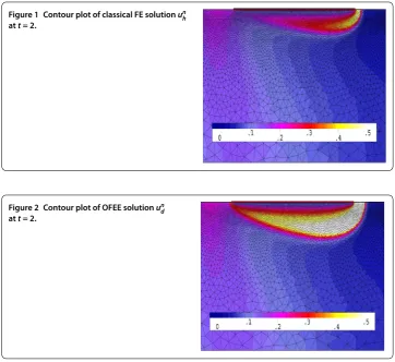
Figure 1 Contour plot of classical FE solutionun h att= 2.
Figure 2 Contour plot of OFEE solutionund att= 2.
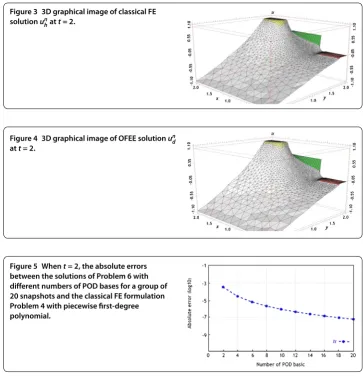
(n= , , . . . , ,i.e., at timet= ., ., . . . , .) for Problem (the classical FE formula-tion) to constitute a set of snapshots. By computing, withd= andk= –, we achieve the error estimation (j=λj)/≤×–in Theorem , which shows that we only need to take six POD bases. Thus, the OFEE format (Problem ) at each time level has only degrees of freedom, while the classical FE formulation (Problem ) contains more than ×degrees of freedom. Therefore, the OFEE format (Problem ) cannot only alleviate the computational load and save time-consuming calculations in the computational pro-cess, but also reduce the accumulation of truncation errors in the computational process. When we solve the OFEE format (Problem ) with six optimal POD bases, according to the seven steps of implementation of the OFEE format in Section ., we find that the OFEE format att= is still convergent, without the need to renew the POD basis. The OFEE solution obtained with the OFEE format (Problem ) is depicted graphically in Figures and . The images in Figures and look very much alike, and so do those in Figures and . Nevertheless, the OFEE solutions are probably better than the classical FE solutions due to the little accumulation of truncated errors of the OFEE format (Problem ) in the computational process.
Figure shows the absolute error between solutionsundof the OFEE format (Prob-lem ) with different numbers of POD bases and the solutionsun
Figure 3 3D graphical image of classical FE solutionun
hatt= 2.
Figure 4 3D graphical image of OFEE solutionun d att= 2.
Figure 5 Whent= 2, the absolute errors between the solutions of Problem 6 with different numbers of POD bases for a group of 20 snapshots and the classical FE formulation Problem 4 with piecewise first-degree polynomial.
This has shown that the OFEE format is feasible and efficient for solving the viscoelastic wave equation.
5 Conclusions
In this article, we use the POD technique to build the OFEE format for the D viscoelastic wave equation. We first extract snapshots from the initial fewL(LN) classical FE so-lutions for the D viscoelastic wave equation. Next, we constitute the POD basis of snap-shots by means of the POD method. Then the FE subspaces of the classical FE format are replaced with the subspaces spanning the most main POD bases to build the OFEE formulation for the D time-dependent conduction-convection problem. Finally, we de-duce the existence, uniqueness, stability, and convergence of the OFEE solutions of the D viscoelastic wave equation and furnish the implement procedure for the OFEE format. Comparing the numerical simulation errors with the theoretical errors we have verified that the theoretical errors are concordant with the computing errors, thus validating both the feasibility and efficiency of the OFEE format.
Acknowledgements
Competing interests
The authors declare that they have no competing interests.
Authors’ contributions
All authors contributed equally and significantly in writing this article. All authors wrote, read, and approved the final manuscript.
Author details
1School of Control and Computer Engineering, North China Electric Power University, No. 2, Bei Nong Road, Changping
District, Beijing, 102206, China. 2School of Mathematics and Physics, North China Electric Power University, No. 2, Bei
Nong Road, Changping District, Beijing, 102206, China.
Publisher’s Note
Springer Nature remains neutral with regard to jurisdictional claims in published maps and institutional affiliations.
Received: 10 August 2017 Accepted: 4 September 2017
References
1. Gurtin, M, Pipkin, A: A general theory of heat conduction with finite wave speeds. Arch. Ration. Mech. Anal.31(2), 113-126 (1968)
2. Lin, YP: A mixed boundary problem describing the propagation of disturbances in viscous media solution for quasi-linear equations. J. Math. Anal. Appl.135(2), 644-653 (1988)
3. Suveika, IV: Mixed problems for an equation describing the propagation of disturbances in viscous media. J. Differ. Equ.19(2), 337-347 (1982)
4. Raynal, M: On some nonlinear problems of diffusion. In: London, S, Staffans, O (eds.) Volterra Equations. Lecture Notes in Math., vol. 737, pp. 251-266. Springer, Berlin (1979)
5. Yuan, Y: Finite difference method and analysis for three-dimensional semiconductor device of heat conduction. Sci. China Math.39(11), 21-32 (1996)
6. Yuan, Y, Wang, H: Error estimates for the finite element methods of nonlinear hyperbolic equations. J. Syst. Sci. Math. Sci.5(3), 161-171 (1985)
7. Xia, H, Luo, ZD: A POD-based optimized finite difference CN extrapolated implicit scheme for the 2D viscoelastic wave equation. Math. Methods Appl. Sci. (2017). doi:10.1002/mma.4499
8. Cannon, JR, Lin, Y: A prioriL2error estimates for finite-element methods for nonlinear diffusion equations with
memory. SIAM J. Numer. Anal.27(3), 595-607 (1999)
9. Li, H, Zhao, ZH, Luo, ZD: A space-time continuous finite element method for 2D viscoelastic wave equation. Bound. Value Probl.2016, Article ID 53, 1-17 (2016)
10. Zokagoa, JM, Soulaımani, A: A POD-based reduced-order model for free surface shallow water flows over real bathymetries for Monte-Carlo-type applications. Comput. Methods Appl. Mech. Eng.221-222, 1-23 (2012) 11. Rozza, G, Veroy, K: On the stability of the reduced basis method for Stokes equations in parametrized domains.
Comput. Methods Appl. Mech. Eng.196, 1244-1260 (2007)
12. Luo, ZD, Zhu, J, Wang, RW, Navon, IM: Proper orthogonal decomposition approach and error estimation of mixed finite element methods for the tropical Pacific Ocean reduced gravity model. Comput. Methods Appl. Mech. Eng.
196(41-44), 4184-4195 (2007)
13. Luo, ZD, Chen, J, Navon, IM, Yang, XZ: Mixed finite element formulation and error estimates based on proper orthogonal decomposition for the non-stationary Navier-Stokes equations. SIAM J. Numer. Anal.47(1), 1-19 (2008) 14. Luo, ZD, Chen, J, Navon, IM, Zhu, J: An optimizing reduced PLSMFE formulation for non-stationary
conduction-convection problems. Int. J. Numer. Methods Fluids60, 409-436 (2009)
15. Luo, ZD, Xie, ZH, Chen, J: A reduced MFE formulation based on POD for the non-stationary conduction-convection problems. Acta Math. Sci.31(5), 765-1785 (2011)
16. Luo, ZD, Du, J, Xie, ZH, Guo, Y: A reduced stabilized mixed finite element formulation based on proper orthogonal decomposition for the non-stationary Navier-Stokes equations. Int. J. Numer. Methods Eng.88(1), 31-46 (2011) 17. Luo, ZD, Li, H, Zhou, YJ, Xie, ZH: A reduced finite element formulation and error estimates based on POD method for
two-dimensional solute transport problems. J. Math. Anal. Appl.385(1), 371-383 (2012)
18. Wang, Z, Akhtar, I, Borggaard, J, Iliescu, T: Proper orthogonal decomposition closure models for turbulent flows: a numerical comparison. Comput. Methods Appl. Mech. Eng.237-240, 10-26 (2012)
19. Ghosh, R, Joshi, Y: Error estimation in POD-based dynamic reduced-order thermal modeling of data centers. Int. J. Heat Mass Transf.57(2), 698-707 (2013)
20. Stefanescu, R, Sandu, A, Navon, IM: Comparison of POD reduced order strategies for the nonlinear 2D shallow water equations. Int. J. Numer. Methods Fluids76(8), 497-521 (2014)
21. Urban, K, Patera, AT: An improved error bound for reduced basis approximation of linear parabolic problems. Math. Comput.83, 1599-1615 (2014)
22. Yano, M: A space-time Petrov-Galerkin certified reduced basis method: application to the Boussinesq equations. SIAM J. Sci. Comput.36(1), A232-A266 (2014)
23. Dimitriu, G, Stefanescu, R, Navon, IM: POD-DEIM approach on dimension reduction of a multi-species host-parasite system. Ann. Acad. Rom. Sci. Ser. Math. Appl.7(1), 173-188 (2015)
24. Liu, Q, Teng, F, Luo, ZD: A reduced-order extrapolation algorithm based on CNLSMFE formulation and POD technique for two-dimensional Sobolev equations. Appl. Math. J. Chin. Univ. Ser. A29(2), 171-182 (2014)
25. Luo, ZD, Li, H: A POD reduced-order SPDMFE extrapolating algorithm for hyperbolic equations. Acta Math. Sci.
34B(3), 872-890 (2014)
27. Luo, ZD, Teng, F: An optimized SPDMFE extrapolation approach based on the POD technique for 2D viscoelastic wave equation. Bound. Value Probl.2017, Article ID 6, 1-20 (2017)
28. Adams, RA: Sobolev Spaces. Academic Press, New York (1975)