The value of reliability

Munich Personal RePEc Archive

The value of reliability

Fosgerau, Mogens and Karlström, Anders

Technical University of Denmark, Royal Institute of Technology,

Sweden

2010

The value of reliability

∗

Mogens Fosgerau

Anders Karlstr¨om

May 10, 2009

Abstract

We derive the value of reliability in the scheduling of an activity of ran-dom duration, such as travel under congested conditions. Using a simple formulation of scheduling utility, we show that the maximal expected utility is linear in the mean and standard deviation of trip duration, regardless of the form of the standardised distribution of trip durations. This insight provides a unification of the scheduling model and models that include the standard deviation of trip duration directly as an argument in the cost or utility func-tion. The results generalise approximately to the case where the mean and standard deviation of trip duration depend on the starting time. An empirical illustration is provided.

KEYWORDS: Welfare; Random duration; Time; Scheduling; Reliability; Vari-ability

JEL codes: D01; D81

∗_{We are grateful to Ken Small, John Bates, Steffen Andersen and seminar participants at the}

University of Copenhagen and the European Transport Conference for comments. We thank Ren´e Ring from the Danish Roads Directorate for supplying data. Mogens Fosgerau has received finan-cial support from the Danish Sofinan-cial Science Research Council. Anders Karlstr¨om was partially financed from the Centre for Transport Studies, Royal Institute of Technology.

†_{Technical University of Denmark, 2800 Kgs. Lyngby, Denmark, Phone: +45 4525 6521, Fax:}

+45 4593 6533, E-mail: [email protected] and Centre for Transport Studies, Royal Institute of Technology, Sweden

‡_{Royal Institute of Technology, SE-100 44 Stockholm, Sweden, Phone: +46 8 790 9263, Fax:}

1

Introduction

In this paper we consider the value of reliability for an agent who wishes to under-take an activity such as a trip of random duration and must decide when to initiate the activity, knowing only the distribution of its duration. We are concerned with the value of changes to the distribution of the trip duration. The value of a change in the mean duration is just the value of time, which is a concept with a long his-tory in economics (Becker,1965;Beesley,1965;Johnson, 1966;DeSerpa,1971)

and there is a large literature on its measurement.1 The concept of the value of

reliability is less well established but about as important. In this paper we take the value of reliability to be the value of a change in the standard deviation of trip

du-ration. Some contributions (Brownstone and Small,2005;Lam and Small,2001;

Small et al., 2005) have instead defined reliability as the range between, e.g., the 0.5 and the 0.9 quantiles of the distribution of durations.

We incorporate reliability by building on the model of Small (1982)2, who

considered the scheduling of commuter work trips when the commuters have

scheduling costs as well as time and monetary costs.3 We formulate the

schedul-ing costs as an opportunity cost per minute of startschedul-ing early and a greater cost per minute of finishing late relative to some fixed deadline. In contrast to earlier

contributions (e.g., Noland and Small, 1995), we are able to derive the optimal

expected cost for a general distribution of trip durations. We obtain the simple result that the optimal departure time as well as the optimal expected cost depend linearly on the mean and standard deviation of the distribution of trip durations, provided the standardised distribution is fixed. Both the optimal departure time and the value of reliability depend in a simple way on the standardised distribu-tion of trip duradistribu-tions and the optimal probability of being late, which in turn is given by the scheduling costs.

In this paper we are able to show that the expected utility is linear in stan-dard deviation for any travel time distribution. We also show that the influence of the travel time distribution on valuation of reliability can be summarised in two factors: the standard deviation and a mean lateness factor, which can easily be calculated for any travel time distribution. This result is useful when one has pref-erence parameters estimated for one travel time distribution (for instance a stated

1_{Some recent references on the measurement of the value of time areSmall et al.(2005) and}

Fosgerau(2007).

2_{The model derives fromVickrey(1969).}

3_{Some early contributions discussing the cost of stochastic delay areDouglas and Miller(1974)}

preference study), and want to use them in an applied context with a different, empirical travel time distribution.

Although originally motivated in transport, the structure of the scheduling problem occurs in many situations; for example, deciding when to enter a queue or when to begin a search. For firms, some inventory stock problems are of similar structure, for instance when holding a deteriorating good in stock is costly, with a random cut-off quality with high cost and costs for delayed delivery (Liaoa et al.,

2000;Hochman et al.,1990). In health economics, waiting times for patients are

random and associated with a cost (Mataria et al., 2007). The structure of the

scheduling problem also occurs in the decision of how durable to design a prod-uct, given that it should last for at least some fixed period and lacking knowledge of the intensity of use. Finally, the timing of activities is also the focus in the literature on the real option model (Dixit and Pindyck,1994). However, while the option value model focuses on the timing of decision under increasing informa-tion, we address a situation where waiting does not allow more information to be gathered. Hence, our problem is not an optimal stopping problem in the sense of the real option model.

In transportation, similar problems occur in several different contexts. Airlines

have to decide how much slack to allow in the scheduling of flights. InBrueckner

(2004), the passenger must buy the air ticket before knowing his preferred

ar-rival time, and expected scheduled delay differs between airlines. The scheduling problem with delays is also relevant in the tourism literature (Batabyal,2007).

Increasingly congested road networks have caused travel times to become highly irregular in many places, which makes road transport an important case for the scheduling model. In this paper we find that travel time uncertainty ac-counts for about 15 per cent of time costs on a typical urban road. Considering the large share of individuals’ time budgets that is spent on transport, it is clear that uncertainty of trip durations represents a significant cost to society in general. The concepts of the value of time and the value of reliability are both of crucial im-portance for decisions regarding capacity provision, operations, pricing and other regulation of transport networks. Both concepts are similarly important in urban economics, travel costs being a main determinant of urban spatial structure (e.g.,

Brueckner,1987).

Transport is also a clear case of time dependent demand with sharp peaks in

the morning and the afternoon. In our empirical illustration in Section 4we test

analysis we also deal with the case where the mean and standard deviation of the distribution of trip durations depend on the departure time. In transport, this pertains to the case where a traveller decides to leave earlier or later along the slopes of the peak in order to avoid the worst. This kind of analysis is important for understanding the effects of pricing policies aimed at regulating traffic during the peak (peak spreading).

As a final application of the model, we consider the case of a scheduled ser-vice, where the departure time cannot be chosen freely, but must adhere to a fixed schedule. We are able to make some progress with this case, but find that the sim-ple properties of the unconstrained case no longer hold. In particular, the expected utility is no longer linear in the standard deviation of trip duration.

It should be noted that we take the individual perspective, where the distribu-tion of trip duradistribu-tions is seen as exogenous. This is in contrast with the literature that investigates the properties of equilibrium where the travel time distribution is dependent on the individual departure time choices, and where individuals

ap-ply scheduling considerations. Notably, there is the bottleneck model of Vickrey

(1969), which has been developed, e.g., in Arnott et al. (1993). A few

contri-butions include stochastic capacity and demand such that travel times become random, e.g., Daniel(1995) andArnott et al.(1999). Furthermore, there is a

lit-erature on learning the equilibrium in congestion games (Sandholm,2002,2005)

that goes some way in handling stochastic delays. However, none of the papers mentioned in this paragraph address the value of reliability.

The layout of the paper is as follows. Section 2 starts with a brief background from the existing transportation literature. Section3does the first bit of theoretical work presenting a simple model where the trip duration distribution is independent

of the departure time. Then Section4measures some characteristics of observed

travel times by car on a typical congested urban road. As this example illustrates, the standardised travel time distribution may be independent of the time of day but the mean and standard deviation are not. Therefore the model is extended

in Section 5 to the cases where the mean and the standard deviation but not the

standardised trip duration distribution depend on departure time as could be the

case through a peak period. Section 6 considers briefly the case of a scheduled

service, where the departure time cannot be chosen freely. Section 7concludes

2

Modelling background

We will first give a short review of the existing transportation literature on the value of reliability. There are basically two existing approaches.

In the first approach (the mean-variance approach), it is assumed that individ-uals have preferences against travel time uncertainty per se. The expected utility of an individual can be written (ignoring monetary cost terms)

E(U) = ηµ+ρσ (1)

whereµis the expected travel time andσ is the standard deviation of travel time,

while η and ρare preference parameters. For applications of this approach, see

Hollander(2006) andNoland and Polak(2002). Some contributions have replaced the standard deviation with another measure of scale, an interquantile range (see e.g., Small et al.,2005, and the references in the introduction).

In the second approach (the scheduling approach), the individual holds

pref-erences for timing of activities, which is more in line with transport demand as a derived demand. Utility is defined directly from outcomes, i.e. being early or late. Travel time variability affects individuals’ utility to the extent that the arrival time at an activity (destination) is affected. The individual holds preferences for being

early or late, compared to a preferred arrival time (PAT), see Small (1982) and

Noland and Small(1995). Normalising an individual’s PAT to be at time zero, let

−Dbe the departure time. Hence, earlier departure corresponds to a largerD.

Let T be the stochastic travel time. Then, in the scheduling approach, the

utility is given by4

U(D, T) = αT +β(T −D)−

+γ(T −D)++θ1T >D,

where (T −D)−

is schedule delay early,(T −D)+ _{is schedule delay late. The}

term θ 6= 0 allows for a discontinuous penalty for lateness. Then the expected

utility is given by

E(U(D)) =αµ+βE(T −D)−

+γE(T −D)++θpL, (2)

wherepLis the probability of being late.

In the case of an exponential travel time distribution,Noland and Small(1995) derive the expected utility given optimal departure time. Written in the form of

4_{The + notation denotes the function, such thatx}+ _{= xifx > 0and zero otherwise,x}− _is

defined byx=_x+

Bates et al.(2001), we have

E(U(D∗

)) =αµ+ ˜H(α, β, γ, θ,∆, σ)σ+θp∗

L (3)

whereσis the standard deviation (and mean) of the exponential travel time

distri-bution, andp∗

Lis the probability of lateness, given optimal departure timeD ∗

. The term∆, definedBates et al.(2001), allows the travel time distribution to depend on departure time to a certain extent.

In many cases, the analysis is simplified by the assumption that θ = 0 and

that the travel time distribution is independent of the departure time (∆ = 0).

Then, Bates et al. (2001) argue that for a wide range of distributions, βE(T −

D∗ )−

+γE(T −D∗

)+ _{is well approximated by H˜(β, γ)σ, where σ is the}

stan-dard deviation of the travel time, andH˜ can be considered constant for any given

combination ofβandγ. They do not provide evidence to support this claim.

The main purpose of this paper is to show that this statement is true in general

and how the factorH can be calculated for any travel time distribution. In

partic-ular, we will show that it is dependent on the shape of the travel time distribution.

3

A simple model

Consider an agent about to undertake a trip of uncertain duration. Express the travel time (duration) in the following convenient form.

T =µ+σX, (4)

where X is a standardised random variable with mean 0, variance 1, densityφ,

and cumulative distribution Φ.5 _{The problem of the agent is to choose when to}

depart given a preferred arrival time. As above, say that his preferred arrival time is 0, and that he departs at time−D.

We assume a utility function consisting of three terms:

U(D, T) =λD+ωT +ν(T −D)+, (5)

where(λ, ω, ν)are preference parameters. The first term is the disutility of start-ing early. We may think of this as the opportunity cost of interruptstart-ing a prior

5_{We have assumed that the mean ofXexists. We also assume thatXhas convex support such}

that the inverse distribution exists. The assumption thatXhas a variance is not strictly necessary.

activity. The second term captures the disutility of time spent travelling. The third term is the disutility of being late. To keep things simple, we do not consider a

cost term. Note that we use a different formulation than the customary(α, β, γ)

formulation in, e.g., Bates et al.(2001) andArnott et al. (1993). Below we shall show that they are in fact equivalent. The main reason is that our formulation makes it explicit how both the value of time and the value of reliability depend on preferences related to activities both earlier and later than the trip under consid-eration. A secondary reason is that our notation reduces clutter in mathematical derivations to follow.

To clarify the translation between our formulation and the customary(α, β, γ) formulation, note that the latter defines the utility function by

U =αT +β(T −D)−

+γ(T −D)+.

Note that

(T −D)−

= (T −D)+−T +D

and this to write the utility function as

U = (α−β)T +βD+ (β+γ)(T −D)+.

Then in our formulation we have

ω = α−β, λ = β, ν = β+γ.

We do not include the discontinuous penaltyθfor being late, nor do we include

any disutility for uncertainty per se. Note that the formulation of utility may be viewed as a minimal way of introducing risk aversion. In general, risk aversion results from concavity of utility. Linear utility results in risk neutrality. In (5),

utility is linear except for the lateness term that has a kink at the point T = D

where lateness kicks in. The results to be derived below will depend crucially on these assumptions, see Bates et al. (2001) for a discussion. Finally, note that the travel time distribution is independent of departure time. This assumption is strong and will be relaxed later in the paper.

We assume that the agent choosesDso as to maximise expected utility, i.e.

EU∗

=max

D EU(D, T) =maxD "

λD+ωµ+ν

Z ∞

D−µ σ

(µ+σx−D)φ(x)dx

#

.

AppendixA.1 shows that the first order condition for the agent’s utility maximi-sation problem is

Φ

D−µ σ

= 1− λ

ν. (7)

We note from (7) that λ/ν is the optimal probability of being late (Bates et al.,

2001). Rewriting the first order condition we find that the optimal departure time

is

D∗

=µ+σΦ−₁

1− λ

ν

. (8)

This shows that the distribution of X only enters the optimal departure time

through its 1− λ_ν quantile. So even though the scheduling utility function has

a kink, the optimally chosen departure time is linear in µ and σ. By inserting

the optimal departure time (8) into the expected utility it is possible to obtain the

optimal maximum expected utility (see appendixA.1).

EU∗

= (λ+ω)µ+νσ

Z 1

1−λ ν

Φ−₁ (s)ds

Now, define the functional

H(φ,λ ν) =

Z 1

1−λ ν

Φ−₁

(s)ds (9)

To interpret H, we note that H is the mean lateness in standardised travel time.

Therefore, we will henceforth termH themean lateness factor.

Given the definition of the mean lateness factor in (9), the expected utility

of an agent who faces a given distribution of trip durations and who optimally chooses his departure time can be written as

EU∗

= (λ+ω)µ+νH(Φ,λ

ν)σ. (10)

First, we identify in the first term(λ+ω)as the the value of travel time. Our model formulation highlights that the value of travel time depends on both the disutility of travel time itself, as well as the marginal disutilityλfrom interrupting a previous activity. The marginal disutility from interrupting a previous activity also affects the valuation of travel time reliability through its influence on the

Second, we observe that the optimal expected utility is linear in the mean and standard deviation of the trip duration, provided the standardised distribution of

durations Φ is constant. It should be emphasised that this holds for any fixed

standardised (absolutely continuous) travel time distribution. This result has been hinted at in the literature, but until now it has only been established in some special cases (Noland and Small,1995;Bates et al.,2001).

Third, the value of reliability,νH(φ,λ

ν), is not a constant preference parameter

but depends on the scheduling parametersλandν, as well as on the standardised

duration distribution φ. In particular, the mean lateness factor depends on the

shape of the travel time distribution above its1− λ_ν quantile.

Before proceeding, we shall state the main result in (10) in terms of the cus-tomary(α, β, γ)parameters. Substituting parameters, the optimal expected utility can be written as

EU∗

=αµ+ (β+γ)H(Φ, β

β+γ)σ

with

H(Φ, β β+γ) =

Z 1

γ β+γ

Φ−₁ (s)ds.

In order to apply the model, one needs to know the preference parameters (ω, λ, ν)or alternatively(α, β, γ)and also the standardised travel time distribution

φ. In some studies the parametersηandρin (1) are estimated directly. However,

under the current model we haveρ = νH which depends not only on preference

parameters but also on the standardised travel time distribution. Therefore, the

ρ parameter cannot be directly applied in a different setting, unless we assume

that the standardised travel time distribution is the same in the first study and the application.6

Our results do indicate how one can translate models estimated in terms of

η and ρ into (ω, λ, ν)-terms. We require knowledge of the standardised travel

time distribution φ prevailing when estimating η and ρ and also knowledge of

the optimal probability of being late λ/ν.7 _{Using this information, we may then}

compute the value ofHthat prevailed in the estimation study. From ρ= νH we

may then find ν and from the optimal probability of being lateλ/ν we may find

λ. Finally, useη=λ+ωto findω.

6_{As an example, the estimates ofη andρinEliasson(2004) have been applied directly in a}

cost benefit analysis of the Stockholm congestion scheme (Eliasson,2009).

7_{One could estimate the average probability of being late from typical stated preference studies}

4

Empirical illustration

In this section we use a travel time dataset to first estimate the mean and stan-dard deviation of travel time as a function of the time of day. Results show that these functions are not constant as was the maintained assumption in the previous

section. The standardised travel time distribution φ does however appear to be

roughly constant over the day. We will use this information to take a look at the

mean lateness factorH.

We use data recorded over the period January 16 to May 8, 2007 at a congested radial road in Greater Copenhagen. Based on timed license-plate matches, the data provide minute by minute observations of the average travel time in minutes for an 11.260 km section. We consider weekdays between 6 AM and 10 PM and discard observations where no traffic was recorded. We use data for the direction towards the city centre, where there is a distinct peak in the morning. This dataset has 24 271 observations. Label these by (Ti, ti), where Ti is travel time in minutes for the i’th observation andti is the time of day in minutes since midnight.

Figure1 shows first a nonparametric kernel regression of travel time against

time of day.8 The resulting curve is an estimate ofµ(t). The figure also shows the 95 per cent pointwise confidence band. It is fairly tight indicating thatµis quite precisely estimated. There is a sharp morning peak at 8 AM and a smaller peak in the afternoon between 4 and 5 PM.

The lower curve estimates the standard deviation of travel time as a function of the time of day, σ(t) = pE[(T −µ(t))2_{]. This is achieved by performing a}

nonparametric regression of squared residuals (Ti −µ(ti))2 against time of day and then taking the square root of the result.9

Using these estimated functions we have computed standardised travel times byXi = (Ti−µ(ti))/σ(ti)such that these have zero mean and unit variance

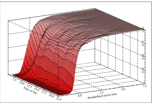
con-ditional on the time of day. Figure 2shows a nonparametric estimate of the

cu-mulative distribution of standardised travel time conditional on the time of day.10 That is, at each time of day, the figure shows an estimate of the cumulative

distri-8_{This regression has been performed using a normal second-order kernel and a bandwidth of}

15 minutes. This is larger than the bandwidth indicated by least squares cross-validation (Li and

Racine,2007) but the regression is visibly undersmoothed by that bandwidth. We note that the

number of observations is large and the independent variable (time of day) is binned by minute

such that the optimal bandwidth might seem to be too small. All programming is in Ox (Doornik,

2001). The code is available on request.

9

The bandwidth is again taken to be 15 minutes, chosen by eye-balling.

10

bution of standardised travel time. If the distribution of standardised travel time is independent of the time of day, then all these curves will be parallel.

A formal test rejects independence of the standardised travel time and time of day. However, that finding should probably not be emphasised too much since the dataset is large and small differences will lead to rejection of independence.

Fig-ure2 does also visually reveal some dependency, especially around the morning

peak, but the figure suggests the dependency is not strong.

We have then estimated the unconditional density of the standardised travel

times.11 The resulting estimate is shown in Figure 3, where the dashed curve

indicates the lower bound of the 95 per cent pointwise confidence interval. The estimated density has a heavy right tail and bears some resemblance to a lognormal or a gamma density, but it is clear from the figure that it is neither.

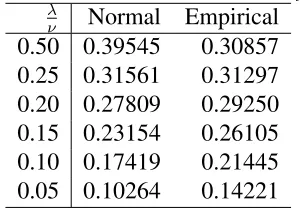
We have computedH(φ,λ

ν)for various values of λ

ν. We have done this both for the empirical distribution of standardised travel times and for the standard normal

distribution. The results are shown in Table 1. In this example there are large

differences in H between the normal and the empirical travel time distribution,

showing the importance of accounting for the actual distribution of durations. The differences are largest for small values of λ_ν when the optimal probability of being late is low. This is due to the fat right tail of the empirical travel time distribution relative to the normal distribution. However, the difference is also quite large when the optimal probability of lateness is one half.

5

Time varying mean and standard deviation of

du-ration

So far we have considered the distribution of travel time to be independent of the departure time. This is not true in general, as the previous section showed. Indeed, in that example, the mean and standard deviation of durations did depend on the departure time, while the distribution of standardised durations could still be assumed to be roughly independent of the departure time.

We will now relax the assumption of fixed mean and standard deviation of trip durations. We will consider a situation where the mean and standard deviation of durations depend linearly on the departure time. In the example considered in the

previous section, we noted that µand σin the example seemed to vary (more or

11_{Using a normal second-order kernel and a bandwidth of 0.18162 chosen by least squares}

less) linearly with the time of day on both sides of the peak. The main motivation for looking at this case is that we are considering small changes such that we may assume that the departure time changes in a continuous fashion. With large changes, travellers may decide to switch from one side of the peak to another in which case the linearity assumption is no longer useful.

We use the following parametrisation where linear functions are pivoted around

the optimal departure time corresponding to constant values ofµandσ.

D0 = µ0+σ0Φ

−₁

1− λ

ν

µ = µ0+µ

′

(D−D0)

σ = σ0+σ

′

(D−D0)

The mathematical derivations for this case are somewhat involved and are given in AppendixA.2. It turns out that the optimal expected utility is still linear in mean duration. That is,

dEU∗

dµ0

= (λ+ω),

which is the same result as in the case where the distribution of durations is in-dependent of the departure time. Thus in computing the marginal expected utility of mean duration we may ignore that the mean and standard deviation functions

depend on the endogenous departure timeD.

The corresponding result for the standard deviation is more complicated. Write the value of reliability, i.e. the derivative of the optimal expected utility with re-spect toσ0, as a function of the slopesµ′ andσ′:

V oR(µ′

, σ′

) = dEU

∗

dσ0

.

Like the value of time, the value of reliability does not depend on the levels of the

mean and standard deviation of duration inµ0andσ0. Define for convenience the

standardised departure timesY = D−_µ

σ andY0 = Φ −1

(1− λ

ν), where the latter is

the optimal departure time in the case of constantµ = µ0 andσ = σ0. Then we

find that the value of reliability is given by

V oR(µ′

, σ′

) =λY0 −νY0(1−Φ(Y)) +ν

Z ∞

Y

xφ(x)dx.

As would be expected, this expression reduces to V oR(0,0) = νR∞

Y0 xφ(x)dx, which is the same result as in Section3. The appendix shows thatV oR(µ′

, σ′

V oR(0,0), such that the value of reliability is overestimated if dependency of the distribution of durations on the departure time is ignored. This is true regardless of the signs ofµ′

andσ′

, so it does not matter whether the upward or the downward slope of a peak is considered.

Using the independence assumption as an approximation may, however, not lead to a large error as can be seen from the following approximation, derived in

AppendixA.2.

V oR(µ′

, σ′

)−V oR(0,0)

V oR(0,0) ≈ − 1 2φ(Y0)H

λ+ω ν µ

′

+Hσ′

2

This formula may be used to correct an estimate of V oR based on constant

µ and σ. If the discrepancy is small we may alternatively just use V oR(0,0)

and ignore the error. For the example in Section4we find the following figures.

Observe from Figure 1that µ′

≈ 10/120 ≈ 0.08and that σ′

≈ 4/120 ≈ 0.03. FromSmall(1982) we take the parameters as roughly(α, β, γ) = (2,1,4). Then

we haveω =α−β = 1,λ=β = 1andν =β+γ = 5.

From Table1we findH ≈0.29. Furthermore,φ(Y0)≈0.23. With these

num-bers it turns out that the relative approximation error is about -0.012, which must be considered small given the precision with which the preference parameters can be estimated.

Given that the approximation error from applying the independence

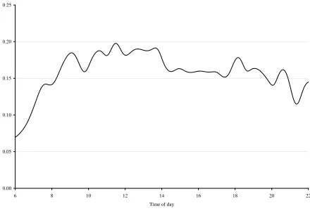
assump-tion is small, we may use (10) to compute the share of the time costs due to

reliability for a traveller in the empirical example in the previous section. Figure4

shows this share over the day. It varies around 15 per cent which must be consid-ered significant. Even so, it is quite conceivable that this share is higher in places with more serious congestion.

6

The case of a scheduled service

preferred completion time and retain the assumption that duration is random given

byµ+σX, whereµandσ are now again fixed. Unfortunately, in this case, as in

Bates et al.(2001), it seems not possible to solve the utility maximisation problem explicitly for general travel time distributions.

Still, it is possible to say something. Consider the expected utility function as a function of departure time D:

EU(D) = λD+ωµ+ν

Z ∞

D−µ σ

(µ+σx−D)φ(x)dx.

This is globally convex since d2EU_dD2(D) = ν σφ(

D−µ

σ ) > 0. The expected utility

maximising departure time will therefore always be the one in the interval defined by the equation

EU(Dh−h) =EU(Dh +h),

since this equation identifies the interval of length2hof maximal expected utility. We have fixed the preferred arrival time at time 0 and taken the scheduling of departure times to be independent of everything else. We may therefore view the scheduling of departure time as a uniformly distributed random variable over the interval[Dh−h, Dh+h]. The expected utility under such a schedule is therefore

given by the following expression.12

E(EU(D)) = 1

2h

Z Dh+h

Dh−h

EU(D)dD

It seems not possible to find a general explicit solution for this for a general dura-tion distribudura-tion. However, it is possible in some cases to deriveE(EU(D))under specific assumptions about the duration distribution. It turns out that the resulting expression forE(EU(D))is rather complex, and in particular it is not in general

linear in the mean and standard deviation of duration. AppendixA.3presents an

example of this for the case of an exponentially distributed travel time.

7

Conclusion

We have established a simple relationship between the fundamental quantities from which cost or disutility is derived in Small’s scheduling model and the mean

12_{Expectation is formed both with respect to the location of the schedule of departure time and}

and standard deviation of a distribution of durations under the optimally chosen departure time. Given the marginal utilities in the scheduling model, it is then possible to compute the value of reliability for any given travel time distribution. Moreover, it is possible to translate the value of reliability from one travel time distribution to another. The result remains a good approximation when the mean and standard deviation of travel time depend on the departure time while the stan-dardised distribution must be constant.

Our analysis is subject to a number of caveats. Most importantly, we assume that the travel time distribution is fixed and known by the decision maker, and we also assume linear scheduling utility with no discontinuous disutility of lateness, nor any disutility of uncertainty per se. The validity of these assumptions needs to be assessed empirically in future research. Whether these assumptions may be relaxed theoretically should also be addressed in future research. We do, however, believe them to be essential for the simple results obtained in this paper. Another important issue, that we have not begun to touch, is the consequences of deviations

from expected utility theory as described by, e.g.,Kahneman and Tversky(1979);

Starmer(2000).

References

Anderson, J. E., Kraus, M., 1981. Quality of service and the demand for air travel. The Review of Economics and Statistics 63 (4), 533–540.

Arnott, R. A., de Palma, A., Lindsey, R., 1993. A structural model of peak-period congestion: A traffic bottleneck with elastic demand. American Economic Re-view 83 (1), 161–179.

Arnott, R. A., de Palma, A., Lindsey, R., 1999. Information and time-of-usage de-cisions in the bottleneck model with stochastic capacity and demand. European Economic Review 43 (3), 525–548.

Batabyal, A., 2007. A probabilistic analysis of a scheduling problem in the eco-nomics of tourism. Ecoeco-nomics Bulletin 12 (4), 1–7.

Becker, G. S., 1965. A theory of the allocation of time. Economic Journal 75 (299), 493–517.

Beesley, M. E., 1965. The value of time spent in travelling: Some new evidence. Economica 32 (126), 174–185.

Brownstone, D., Small, K., 2005. Valuing time and reliability: assessing the evi-dence from road pricing demonstrations. Transportation Research Part A: Pol-icy and Practice 39 (4), 279–293.

Brueckner, J., 1987. The structure of urban equilibria: A unified treatment of the muth-mills model. In: S.Mills, E. (Ed.), Handbook of Regional and Urban Economics, Vol. 2. North Holland, pp. 821–845.

Brueckner, J., 2004. Network structure and airline scheduling. Journal of Indus-trial Economics 52 (2), 291–312.

Daniel, J. I., 1995. Congestion pricing and capacity of large hub airports: A bot-tleneck model with stochastic queues. Econometrica 63 (2), 327–370.

DeSerpa, A. C., 1971. A theory of the economics of time. The Economic Journal 81 (324), 828–845.

Dixit, A., Pindyck, R., 1994. Investment Under Uncertainty. Princeton University Press, Princeton, NJ.

Doornik, J. A., 2001. Ox: An Object-Oriented Matrix Language. Timberlake Con-sultants Press, London.

Douglas, G. W., Miller, J. C., 1974. Quality competition, industry equilibrium, and efficiency in the price-constrained airline market. American Economic Re-view 64 (4), 657–669.

Eliasson, J., 2004. Car drivers’ valuations of travel time variability, unexpected delays and queue driving. European Transport Conference.

Eliasson, J., 2009. A cost-benefit analysis of the stockholm congestion charging system. Transportation Research Part A 43 (4), 468–480.

Hochman, E., Leung, P., W.Rowland, L., A.Wyban, J., 1990. Optimal schedul-ing in shrimp mariculture: A stochastic growschedul-ing inventory problem. American Journal of Agricultural Economics 72 (2), 382–393.

Hollander, Y., 2006. Direct versus indirect models for the effects of unreliability. Transportation Research Part A 40 (9), 699–711.

Johnson, M. B., 1966. Travel time and the price of leisure. Western Economic Journal 4 (2), 135–145.

Kahneman, D., Tversky, A., 1979. Prospect theory: An analysis of decision under risk. Econometrica 47 (2), 263–292.

Lam, T. C., Small, K., 2001. The value of time and reliability: Measurement from a value pricing experiment. Transportation Research Part E: Logistics and Transportation Review 37 (2-3), 231–251.

Li, Q., Racine, J. S., 2007. Nonparametric Econometrics: Theory and Practice. Princeton University Press, Princeton and Oxford.

Liaoa, H.-C., Tsaib, C.-H., Su, C.-T., 2000. An inventory model with deteriorat-ing items under inflation when a delay in payment is permissible. International Journal of Production Economics 63 (2), 207–214.

Mataria, A., Luchini, S., Daoud, Y., Moatti, J.-P., 2007. Demand assessment and price-elasticity estimation of quality-improved primary health care in palestine. Health Economics 16 (10), 1051–1068.

Noland, R. B., Polak, J. W., 2002. Travel time variability: a review of theoretical and empirical issues. Transport Reviews 22 (1), 39–54.

Noland, R. B., Small, K. A., 1995. Travel-time uncertainty, departure time choice, and the cost of morning commutes. Transportation Research Record 1493, 150– 158.

Sandholm, W. H., 2002. Evolutionary implementation and congestion pricing. Re-view of Economic Studies 69 (3), 667–689.

Small, K., 1982. The scheduling of consumer activities: Work trips. American Economic Review 72 (3), 467–479.

Small, K. A., Winston, C., Yan, J., 2005. Uncovering the distribution of motorists’ preferences for travel time and reliability. Econometrica 73 (4), 1367–1382.

Starmer, C., 2000. Developments in non-expected utility theory: The hunt for a descriptive theory of choice under risk. Journal of Economic Literature 38 (2), 332–382.

Vickrey, W. S., 1969. Congestion theory and transport investment. American Eco-nomic Review 59 (2), 251–261.

A

Mathematical appendix

A.1

A simple model

This appendix refers to section3. The first point is to find the first order condition

for the maximisation of the expected utility in (6). Recall the following general

formula:

d dx

Z b(x)

a(x)

f(x, t)dt=b′

(x)f(x, b)−a′

(x)f(x, a) + Z b(x)

a(x)

df(x, t)

dx dt.

Use this to differentiate (6) with respect to the departure time D and set to zero to find the first order condition. Note here that the derivative with respect to the lower integral limit is zero, since the integrand is zero at the lower bound. The derivative with respect to the upper integral limit is also zero, since the upper integral limit is constant. The first order condition then becomes

λ=ν

1−Φ

D−µ σ

.

optimal expected utility.

EU∗

= λ

µ+σΦ−1

1− λ

ν

+ωµ+ν

Z ∞

Φ−1(₁−λ ν)

σx−σΦ−1

1− λ

ν

φ(x)dx

= (λ+ω)µ+λσΦ−₁

1−λ

ν

−νσΦ−₁

1− λ

ν

Z ∞

Φ−1(₁₋λ ν)

φ(x)dx+νσ

Z ∞

Φ−1(₁₋λ ν)

xφ(x)dx

= (λ+ω)µ+λσΦ−₁

1−λ

ν

−νσΦ−₁

1− λ

ν 1−Φ

Φ−₁

1− λ

ν

+νσ

Z ∞

Φ−1(₁₋λ ν)

xφ(x)dx

= (λ+ω)µ+νσ

Z 1

1−λ ν

Φ−1 (s)ds

A.2

Approximation to the value of reliability

This appendix refers to Section 5where the mean and standard deviation of

du-ration are linear in the departure time. We define standardised departure time

Y = D−µ

σ and Y0 = Φ −₁

(1− λ

ν). The first-order condition for the choice of

departure time can be expressed in compact form.

0 = λ+ωµ′

+ν

Z ∞

Y (µ′

+σ′

x−1)φ(x)dx

It is only Y in this expression that depends on µ0 and σ0. So we can conclude

that the derivatives of Y with respect toµ0 and σ0 are zero. This insight allows

us to derive the marginal expected utilities ofµ0 andσ0. Multiply the first-order

condition byD−D0 and subtract from the expected utility (6) to obtain

EU∗

= λD0+ωµ0+ν

Z ∞

Y

(µ0 +σ0x−D0)φ(x)dx

= (λ+ω)µ0+λσ0Y0−νσ0Y0(1−Φ(Y)) +νσ0

Z ∞

Y

xφ(x)dx

We find that dEU_dµ0∗ = (λ+ω)for any value ofµ′

, σ′

. This is the same result as in

The next point is to find the value of reliability. Differentiate the expected utility above with respect toσ0 to obtain

dEU∗

dσ0

= λY0−νY0(1−Φ(Y)) +ν

Z ∞

Y

xφ(x)dx

Recall that the value of reliability isνR∞

Y0 xφ(x)dxin the case whenµ ′

=σ′

= 0

and note that the expression above reduces to this when µ′

= σ′

= 0. As an

approximation to dEU_dσ0∗ it is natural to consider using νR∞

Y0 xφ(x)dx since this does not require computation of Y. It is therefore of interest to consider the size of the error in using such an approximation

Denote the value of reliability byV oR(µ′

, σ′

) = dEU∗

dσ0 . We are then concerned

with the relative difference V oR(µ_{V oR}′,σ′)₍₀−_,V oR₀₎ (0,0) and we would like to show that this is small whenµ′

, σ′

are small.

We may obtain from the FOC that

dY dµ′(µ

′

=σ′

= 0) =− λ+ω

νφ(Y0)

<0

and

dY dσ′(µ

′

=σ′

= 0) =−

R1

1−λ ν Φ

−₁ (s)ds φ(Y0)

<0.

Letz1be one ofµ′, σ′. Then

dV oR dz1

=−ν(Y −Y0)φ(Y)

dY dz1

.

This is zero atµ′

=σ′

= 0since then Y =Y0. Hence the change in the marginal

utility of standard deviation is small when µ′

, σ′

are small. Differentiate again to find

d2_{V oR}

dz1dz2

=−νφ(Y)dY

dz1

dY dz2

−ν(Y −Y0)φ

′

(Y)dY

dz1

dY dz2

−ν(Y −Y0)φ(Y)

d2_Y

dz1dz2

.

At Y = Y0 this equals −νφ(Y0)_dz1dY dY_dz2 < 0, so the value of reliability is locally

concave in z with a local maximum at z = 0. This means that the value of

reliability atz 6= 0is overestimated by using the value atz = 0, regardless of the signs ofz.

Given that we will be making a systematic error by using the formula derived

value of reliability atY0at small values ofz. Using a quadratic approximation we

find that

V oR(µ′

, σ′

)−V oR(0,0)

V oR(0,0) ≈

1

2V oR(0,0)

d2_{V oR}

dµ′2 µ ′₂

+ 2d

2_{V oR}

dµ′_dσ′µ ′

σ′

+d

2_{V oR}

dσ′2 σ ′₂

= −νφ(Y0)

2νH

dY dµ′µ

′

+ dY

dσ′σ ′

2

= − 1

2φ(Y0)H

λ+ω ν µ

′

+Hσ′

2

.

A.3

Example with a scheduled service

This appendix presents an example of a scheduled service with an exponentially

distributed duration, where T = µ+X and X ∼ φ(x) = ξe−ξx_{. We note that}

Φ(x) = 1−e−_ξx

and thatΨ(x) := Rx

0 xφ(x)dx = 1−e−ξx

ξ −xe

−_ξx

. Then it may

be verified that (ω = 0andλ= 1are omitted)

EU(D) = D+ν

ξe

−ξ(D−µ)_.

Moreover the midpoint of the interval from which departure time is chosen is

µ+1

ξlog( ν

2ξh(e

ξh₋

e−ξh )),

such that the expected expected utility becomes

E(EU(D)) = (µ+1

ξ) +

1

ξlog( ν

2ξh(e

ξh_−e−_ξh )).

We may interpret the first term as relating to the mean duration while the second term relates to the standard deviation of duration 1_ξ. But we note that the parameter

ξthat characterizes the exponential distribution also appears inside a complicated

6 7 8 9 10 11 12 13 14 15 16 17 18 19 20 21 22

12.5

15.0

17.5

20.0

Mean travel time

6 7 8 9 10 11 12 13 14 15 16 17 18 19 20 21 22

2

3

4

5

Std.dev. of travel time

Time of day

Tim e of d_ay

Standardised travel time 7.5

10.0 12.5

15.0 17.5

20.0

22.5 0.0

2.5

5.0 7.5

0.25

0.50

0.75

1.00

-2.0 -1.5 -1.0 -0.5 0.0 0.5 1.0 1.5 2.0 2.5 3.0 3.5 4.0 4.5 5.0 0.1

0.2 0.3 0.4 0.5 0.6 0.7

Standardised travel time

0.00 0.05 0.10 0.15 0.20 0.25

6 8 10 12 14 16 18 20 22 Time of day

Table 1:Hat various values of λ_ν λ

ν Normal Empirical

0.50 0.39545 0.30857

0.25 0.31561 0.31297

0.20 0.27809 0.29250

0.15 0.23154 0.26105

0.10 0.17419 0.21445