To pool or not to pool: a partially heterogeneous framework

Munich Personal RePEc Archive

To pool or not to pool: a partially

heterogeneous framework

Sarafidis, Vasilis and Weber, Neville

The University of Sydney, Monash University

8 December 2009

Online at

https://mpra.ub.uni-muenchen.de/36155/

A Partially Heterogeneous Framework for

Analyzing Panel Data

Vasilis Sara…dis

University of Sydney

Neville Weber

University of Sydney

This version: May 2011

Abstract

This paper proposes a partially heterogeneous framework for the analysis

of panel data with …xedT. In particular, the population of cross-sectional

units is grouped into clusters, such that slope parameter homogeneity is

maintained only within clusters. Our method assumes no a priori

infor-mation about the number of clusters and cluster membership and relies on

the data instead. The unknown number of clusters and the corresponding

partition are determined based on the concept of ‘partitional clustering’,

using an information-based criterion. It is shown that this is strongly

con-sistent, i.e. it selects the true number of clusters with probability one as

N _{! 1}. Simulation experiments show that the proposed criterion performs

well even with moderateN and the resulting parameter estimates are close

to the true values. We apply the method in a panel data set of commercial

banks in the US and we …nd …ve clusters, with signi…cant di¤erences in the

slope parameters across clusters.

Key Words: partial heterogeneity, partitional clustering, exploratory

data analysis, information-based criterion, model selection.

JEL Classi…cation: C13; C33; C51.

We are grateful to Genliang Guan for excellent research assistance. We have also bene…ted from helpful comments by Geert Dhaene, Daniel Oron, Tom Wansbeek, Yuehua Wu and seminar participants at the Erasmus University Rotterdam, University of Leuven, University of York and the Tinbergen Institute. Financial support from the Research Unit of the Faculty of Economics and Business at University of Sydney is gratefully acknowledged.

y_{Corresponding author. Faculty of Economics and Business, University of Sydney, NSW}

2006, Australia. E-mail: vasilis.sara…[email protected].

z_{School of Mathematics and Statistics, University of Sydney, NSW 2006, Australia. E-mail:}

1

Introduction

Slope parameter homogeneity is often an assumption that is di¢cult to justify in

panel data models, both on theoretical grounds and from a practical point of view. On the other hand, the alternative of imposing no structure on how these coe¢-cients may vary across individual units may be rather extreme. This argument is

in line with evidence provided by a substantial body of applied work. For exam-ple, Baltagi and Gri¢n (1997) reject the hypothesis of coe¢cient homogeneity in a panel of gasoline demand regressions across the OECD countries, and Burnside (1996) rejects the hypothesis of homogeneous production function parameters in

a panel of US manufacturing industries. Even so, both studies show that fully

heterogeneous models lead to very imprecise estimates of the parameters, which in some cases have even the wrong sign. Baltagi and Gri¢n notice that this is the case despite the fact that there is a relatively long time series in the panel

to the extent that the traditional pooled estimators are superior in terms of root mean square error and forecasting performance. Furthermore, Burnside suggests that in general his estimates show signi…cant di¤erences between the homogeneous and the heterogeneous models and the conclusions about the degree of returns to

scale in the manufacturing industry would heavily depend on which one of these two models is used. Along the same line Baltagi, Gri¢n and Xiong (2000) place the debate between homogeneous versus heterogeneous panel estimators in the context of cigarette demand and conclude that even with a relatively large

num-ber of time series observations, heterogeneous models for individual states tend to produce implausible estimates with inferior forecasting properties, despite the fact that parameter homogeneity is soundly rejected by the data. As pointed out by Browing and Carro (2007), there is usually a lot more heterogeneity than what

empirical researchers allow for in econometric modelling, although the level of het-erogeneity and how one allows for it can make a large di¤erence for outcomes of interest.

These …ndings indicate that the modelling framework of slope parameter

homo-geneity (pooling) and full heterohomo-geneity may be polar cases, and other intermediate

cases may often provide more realistic solutions in practice. The pooled mean

group estimator (PMGE) proposed by Pesaran, Shin and Smith (1999) bridges the gap between pooled and fully heterogeneous estimators by imposing partially

be individual-speci…c and restricts the long-run coe¢cients to be the same across

individuals for reasons attributed to budget constraints, arbitrage conditions and common technologies.

In this paper we propose a modelling framework that imposes partially het-erogeneous restrictions not with respect to the time dimension of the panel, as

PMGE does, but with respect to the cross-sectional dimension, N. In particular,

the population of cross-sectional units is grouped into distinct clusters, such that within each cluster the slope parameters are homogeneous and all intra-cluster

heterogeneity is attributed to a function of unobserved individual-speci…c and/or time-speci…c e¤ects. The clusters themselves are heterogeneous, that is, the slope parameters vary across clusters.

Naturally, the practical issue of how to group the individuals into clusters is

central in the paper. If there is a priori information about cluster membership and the number of clusters, the problem reduces to a split-sample standard panel data regression. In many cases, while it might be plausible to think of a set of factors to which slope parameter heterogeneity can be attributed, such as di¤erences

in tastes, beliefs, abilities, skills or constraints, these are often unobserved and moreover provide no guidance as to what the appropriate partitioning is, or how many clusters exist. In addition, there are often several ways to partition the sample and while the formed clusters may be economically meaningful, they may

not be optimal from a statistical point of view.

Clustering methods have already been advocated in the econometric panel data literature by some researchers; for instance, Durlauf and Johnson (1995) propose clustering the individuals using regression tree analysis, and Vahid (1999) suggests

a classi…cation algorithm based on a measure of complexity using the principles of minimum description length and minimum message length, which are often

employed in coding theory.1 _{Both these methods are based on the concept of}

hierarchical clustering, which involves building a ‘hierarchy’ from the individual units by progressively merging them into larger clusters. The proposed algorithms

provide a consistent estimate of the true number of clusters for T _{! 1} only.

On the contrary, this paper proposes estimating the unknown number of clusters

and the corresponding partition based on the concept of partitional clustering. In

1_{Kapetanios (2006) proposes an information criterion, based on simulated annealing, to}

particular, the underlying structure is recovered from the data by grouping the

individuals into a …xed number of clusters using an initial partition, and then re-allocating each individual into the remaining clusters until the …nal preferred partition minimises an objective function. In this paper the residual sum of squares (RSS) of the estimated model is used as the objective function. The number of

clusters is determined by the clustering solution that minimises RSS subject to a penalty function that is strictly increasing in the number of clusters. Intuitively our procedure is identical to a standard model selection criterion method, although the

study of the asymptotics is more complicated because the number of individuals

contained in a given cluster may vary with N. It is shown that the proposed

criterion is strongly consistent, i.e. it estimates the true number of clusters with

probability one as N grows, for any T …xed. This is important because most

frequently panel data sets entail a large number of individuals and a small number

of time series observations. Furthermore, it is usually the case of smallT where

some kind of pooling provides substantial e¢ciency gains over full heterogeneity. As with other clustering procedures, our method relies on the data to suggest

any clustering structure that might exist, and as such it can be described as an exploratory data analysis approach. Hence, it can be particularly useful when there is no a priori information about the clustering structure, or when one is interested in examining how far a structure that might be meaningful according

to some economic measure lies from the structure that …ts the data best.

The remainder of the paper is as follows. The next section formulates the prob-lem. Section 3 analyses the properties of the proposed clustering criterion. Section 4 discusses the implementation of the algorithm used to implement the

cluster-ing procedure. The …nite-sample performance of the algorithm is investigated in Section 5 using simulated data. Section 6 applies our partially heterogeneous framework to a random panel of 551 banking institutions operating in the US, each observed over a period of 15 years. Five clusters are found and the results

2

Model Speci…cation and Cluster

Determina-tion

We consider the following panel data model:

y!it = 0!x!it+u!it; (1)

wherey!it denotes the observation on the dependent variable for theith individual

that belongs to cluster! at timet, _! = ( _!1; :::; _!K)0 is a K 1vector of …xed coe¢cients, x!it = (x!it1; :::; x!itK)0 is a K 1 vector of covariates, and u!it is a

disturbance term. Therefore, each cluster has its own regression structure with

! = 1; :::; 0, i[₂!] = 1; :::; N!, and t = 1; :::; T. This means that the total

number of clusters equals 0, the!th cluster hasN! individuals, for which there

are T time series observations available. The total number of individuals in all

clusters equals N =P 0

!=1N! and the total sample size is given by S =N T. If the true number of clusters and the corresponding partition or membership

of individualiinto cluster!are both known, the problem reduces to a split-sample standard panel data regression, which is straightforward enough to estimate. In

this paper we are interested in estimating the vector _! for ! = 1; :::; 0, when

neither the true number of clusters nor cluster membership are known.

Unfortu-nately, ignoring cluster-speci…c slope parameter heterogeneity by pooling the data

will not provide a consistent estimate of = P 0

!=1

N!

N !, which is the natural

weighted average value of the cluster-speci…c coe¢cients with weights determined by the proportion of individuals belonging to each cluster. This holds true even

under strict exogeneity of the regressors.

To see this, let E(u!itjx!i1; :::;x!iT) = 0 and N!1 N!

X

i=1

X0

!iX!i p

! MXX;!, a

…nite and positive de…nite matrix, whereX!i = (x!i1; :::;x!iT)0. The pooled

b_pooled = " ₀ X !=1 N! X i=1

X_!i0 X!i

# 1"

0 X !=1 N! X i=1

X_!i0 y!i

# = " ₀ X !=1 N! X i=1

X_!i0 X!i

# 1 0 X !=1 N! X i=1

X_!i0 X!i

! _N! X

i=1

X_!i0 X!i

! 1 _N !

X

i=1

X_!i0 y!i

! = 0 X !=1 " ₀ X !=1 N! N 1 N! N! X i=1

X_!i0 X!i

!# 1"

N! N 1 N! N! X i=1

X_!i0 X!i

!# b_! = 0 X !=1 c

W!b!. (2)

The expression above shows thatb_pooledis a matrix-weighted average of the cluster-speci…c estimates, where the weights are inversely proportional to the cluster

co-variance matrices. Therefore, lettingN!=N !c! , bpooled converges in probability

to

b_pooled p

!

0

X

!=1

W! !, (3)

where W! =

" ₀ X

!=1

c!MXX;!

# 1

[c!MXX;!]. The pooled least-squares estimator is

not consistent for unless, say, the limiting matrix MXX;! is constant across

clusters. The condition MXX;! = MXX is unnatural in economic data sets and

therefore it is unlikely to hold true in most empirical applications.2

Our aim is to try to determine whether a clustering structure can be identi…ed among individuals without utilising a priori information, but rather by relying on

the data to suggest any possible groups. Let us denote the true partition of theN

individuals into 0 clusters by 0 =fC

0

1; : : : ; C00g, whereC

0

! is a set of indices of

elements in the !th _{cluster such that C}0

! =f!1; : : : ; !N0!g f1;2; : : : ; Ng: Thus, the number of individuals in the!th _{cluster isjC}0

!j=N0!, andN01+: : :+N0 0 =

N.

The model under the true partition will be expressed as follows:

yC0

!it =

0

0!xC0

!it+uC!it0 , uC!it0 =

0

C0

!it t+"C!it0 , (4)

2_{Fernandez-Val (2005) and Graham and Powel (2009) study the estimands of linear panel}

or, in matrix form,

YC0

! =XC0! 0!+uC!0,uC!0 = (IN0! ) C!0 +"C!0, (5) whereYC0

! = y

0

!1; :::;y

0

!N_0!

0

, withy!i = (y!i1; :::; y!iT)

0

, is the(N0!T) 1vector

of observations on the dependent variable for the individuals in the !th _cluster,

XC0

! = x

0

!1; :::;x

0

!N_0!

0

, with x!i = (x!i1; :::;x!iT)

0

, is the (N0!T) K matrix of

covariates and 0! is a vector of …xed coe¢cients speci…c to each cluster.

The error term is subject to a factor structure where = ( ₁; :::; _T)0 is a

T r matrix of unobserved common factors and C0

! =

0

!1; :::;

0

!N₀!

0

is a

N0!r 1 vector of factor loadings. Thus, the error allows for individual-speci…c

unobserved heterogeneity, captured by !i, that varies over time in an

intertem-porally arbitrary way, albeit in a similar fashion across i. It also allows for the presence of common unobserved shocks (such as technological shocks and …nancial crises), captured by _t, the impact of which is di¤erent for each individuali. Both cases can be thought of as generating cross-sectional dependence. The composite

error term reduces to the usual two-way error components model by settingr = 2,

t = (1; t)

0

and !i = ( i;1)

0

. The unobserved factors, _t, could be correlated

with x!it and to allow for such a possibility the following speci…cation for the

covariates will be considered:

XC0

! = (IN0! ) C!0 +VC!0, (6)

where C0

! is a N0!r K matrix of factor loadings and VC!0 is a (N0!T) K

matrix containing the idiosyncratic errors of the covariates, which are distributed

independently of the common e¤ects and acrossi.

Pre-multiplying(5)by the transformation matrixQC0

! =IN0!T IN0! (

0 ₎ 1 0

that eliminates the factor structure yields

QC0

!YC!0 =QC!0XC!0 0!+QC0!"C!0, (7) or

e

YC0

! =XeC!0 0!+e"C!0, (8) where YeC0

! =QC!0YC!0, XeC!0 =QC!0VC!0, and so on.

Suppose we partition the population into clusters (N) = nC(N₁); :::; C(N)o

and assume the true number of clusters is bounded by some constant . For ease

of notation we will drop the (N) superscript unless there is ambiguity. Let b _!

be the least squares estimate of based on the observations in the true cluster

C0

! and b!jj be the least squares estimate based on the observations in cluster

C !\Cj0, ! = 1; :::; , j = 1; :::; 0. Let

RSS! = YeC ! XeC !b ! 2

denote the sum of the squares of the residuals for the C ! cluster, and

RSS =RSS( ) =X

!=1

RSS!.

De…ne

FN (!N) =Nlog

RSS

N T +f( ) N, (9)

wheref( ) is a strictly increasing function of and N is a sequence of constants

the size of which depends on N. For example, we often take N =

p

N and f

as the identity function. We propose estimating the number of clusters and the corresponding partition by minimising the following objective function:

FN (_bN)

0 = min1 min(N)FN

(N)

, (10)

where b0 is the value of that minimises FN. It will be shown in the following

section that, under certain conditions, this criterion identi…es 0 with probability

one as N grows large.

Using the above criterion to compare two distinct partitions we have

FN (N) FN (N₀)

= Nlog 1 +RSS( ) RSS( 0)

RSS( 0)

+ [f( ) f( 0)] N;

RSS( ) RSS( 0)

RSS( 0)=N

+ [f( ) f( 0)] N:

The residual sum of squares for the 0 partition divided byN, which appears in

the denominator of the ratio in the expression above, is a measure of the variability in the data. Thus, heuristically, the …rst term compares the goodness of …t of a model normed by a measure of the overall level of spread. Therefore, the proposed criterion is invariant to the scale of the data. This is important because in practice

for any …xedN and T, multiplying the variables by a constant scalar will change

clusters and therefore it tends to over-parameterise the model by allowing for more

clusters than may actually exist. Hence, the penalty acts essentially as a …lter to ensure that the preferred clustering outcome partitions between rather than within clusters. The intuition of the procedure is identical to a standard model selection criterion, although the study of the asymptotics is more complicated in the present

case because the number of individuals contained in a given cluster may vary with

N.

3

Asymptotic Properties of Clustering Criterion

The following assumptions are required to establish the asymptotic properties of

the proposed clustering criterion:

A.1 There exists a …xed constant, 0 < c! < 1, with P!=10 c! = 1, such that

N!=N !c! for != 1; :::; 0, asN ! 1.

A.2 0 is a …xed unknown integer, such that 0 < 0 , where is …xed and

known.

A.3 Given the covariatesX!itcorresponding to the observations in the!thcluster,

the error vectors "_!i = ("!i1; :::; "!iT)0 for the individuals in the cluster are

independent and identically distributed random vectors with mean vector0

and for some > 0, E_j"!itj2+ < 1. To avoid trivialities assume some

elements of"!i have non-zero variance.

Let C` denote a true class or a subset of a true class with N` elements. Given

the matrixXeC`, letXe (t)

C` be the submatrix consisting of rows t; t+T; :::; t+

(N` 1)T of XeC` for t= 1; :::; T.

A.4 There exist constants 1 > 0 and 2 > 0 such that the eigenvalues of

N_` 1Xe0

C`XeC` and N 1

` Xe

(t)0

C` Xe (t)

C` lie in [ 1; 2] for N` large enough.

A.5 For any column vector x!` of XeC`, its elements x

(1)

!`; :::; x

(N`T)

!` satisfy the

condition

N`T

X

i=1

x(_!`i) 2+ =Op

h

(x0<sub>!`</sub>x!`)(2+ )=2=log (x0!`x!`)1+

i

(11)

A.1 ensures that no clusters are asymptotically negligible. In particular, it

implies that for the true partition there exist …xed constants d! 2 (0;1) such

that d! < N_N0! < 1, ! = 1; :::; 0 for N large enough. Assumption A.2 ensures

that the total number of clusters is bounded by a known integer, .3 _Assumption

A.3 is common in panel data models and implies that the covariates are strictly

exogenous with respect to the idiosyncratic error component, "!i, although not

with respect to the total error term. Observe also that "!it is permitted to be

serially correlated in an arbitrary way and heteroskedastic across clusters and

over t. Assumptions A.4 A.5 describe the behaviour of the covariates. A.4 is

employed for identi…cation purposes and ensures that N_` 1Xe0

C`XeC` 1

exists in probability for all N! su¢ciently large.

For any set C` which is a true cluster, a subset of a true cluster or a union of

subsets of a true cluster with _jC`j=N`, let PXe_C` denote the projection matrix

PXe<sub>C`</sub> =XeC` Xe

0

C`XeC` 1

e

X_C0_`, (12)

based on the correspondingXeC` matrix. Let"C` denote the vector of correspond-ing error terms. The followcorrespond-ing lemma controls the rate of growth of a weighted sum of random variables.

Lemma 1 Let$1; $2; :::be a sequence of independent random variables with zero

mean, such that 0< E($2

i) = 2i and Ej$ij2+ < <1 for some >0, >0 and i = 1;2; ::: Furthermore, let 1; 2; :::;2 R be a sequence of constants such

that

(i) B_N2 =

N

X

i=1 2

i ! 1;

(ii)

N

X

i=1

j ij2+ = Op

n

B_N2+ logB_N2 1 o, for some >0.

Then, for N _{! 1}

TN = N

X

i=1

i$i =O BN2 log log BN2

1 2 _a.s.

Proof. See Shao and Wu (2005), Lemma 3.5.

Write

"C` = (1)

C` +:::+ (T)

C` , (13)

where the ith _{element of} (t)

C` is ("C`)iI(i2 ft; t+T; t+ 2T; :::g). For example,

(1)

C` = ("!11;0; :::;0; "!21;0; :::; "!N`1;0; :::;0)

0

and so on. The non-zero elements of the vector (_Ct)_` are the i:i:d:error terms corresponding to the observations at time

t for the elements in the cluster. We can write

"0_C

`PXe<sub>C`</sub>"C` =

T X t=1 T X s=1 (t)0

C`PXe<sub>C`</sub> (s)

C`. (14)

Using the idempotent nature of the matrix PXe_C` and the Cauchy-Schwartz

in-equality we have

(t)0

C`PXe<sub>C`</sub> (s)

C` 2

= (_Ct)_`0P_X2_e

C` (s)

C` 2

= PXe_C`

(t)

C`

0

PXe_C`

(s)

C` 2

(t)0

C`PXe<sub>C`</sub> (t)

C`

(s)0

C` PXe<sub>C`</sub> (s)

C` . (15)

Thus, if (_Ct_{`</sub>)0PXe<sub>C`}

(t)

C` =O(log logNC`)a.s. for eacht, then"

0

C`PXe<sub>C`</sub>"C` =O(log logNC`) a.s.

Applying Lemma 1 along with assumptions CA.1-CA.3 we have

(t)0

C`XeC` =O(N`log logN`)

1

2 _{a.s. (16)}

Therefore,

"0_C

`XeC` =O (N`log logN`)

1

2 a.s. (17)

Furthermore, A.4 ensures that the elements of Xe0

C`Xe

0

C` 1

areO N_` 1 . Hence,

using (16) and arguing as in the proof of Lemma A.2 of Bai, Rao and Wu (1999)

we have

(t)0

C`PXe<sub>C`</sub> (t)

C` = (t)0

C`XeC` Xe

0

C`XeC` 1

e

X_C0_{`</sub> (<sub>C</sub>t<sub>`})

= O(log logN`) a.s. (18)

As a result,

"0_C

`PXe<sub>C`</sub>"C` =O(log logN`) a.s. (19)

The results in (17) and (19) are key to proving that the clustering algorithm

converges to the true number of clusters. The asymptotics are developed by

con-sidering class growing sequences. That is, we will assume that asN increases, the

sequence of true partitions of _f1;2; :::; N_g is naturally nested, i.e.

In other words, the asymptotics can be conceived via a ‘class-growing sequence’

approach, which assigns the (N + 1)th _{observation to any cluster of the previous}

partition based on the …rst N observations. The following theorem shows that

the criterion in (10) selects the true number of clusters amongst all class-growing

sequences with probability one forN large enough:

Theorem 2 Let limN!1N 1 N = 0 and limN!1(log logN) 1 N = 1.

Sup-pose that assumptions A.1-A.5 hold and ₀ is the true clustering partition corre-sponding to model(5). Then the clustering criterion in(10) is strongly consistent that is, it selects 0, the true number of clusters among all class-growing

se-quences, with probability one asN _{! 1}.

Proof. See Appendix.

The …rst condition in Theorem 2 prevents estimating too many clusters as-ymptotically while the second condition prevents under-…tting. Similar conditions

underlie well-known model selection criteria such as the AIC and the BIC, except that the criterion above is developed for the purpose of clustering individuals. Our class-growing approach is motivated by Shao and Wu (2005), who prove consis-tency of a similar criterion function for the cross-sectional regression model. Our

model is more general, while it permits cross-sectional dependence in the errors and arbitrary forms of residual serial correlation. Moreover, the proposed criterion is invariant to the scale of the data.

In practice the unknown in the transformation matrix Q! can be replaced

by any consistent estimator b for …xed T. For example, given that the covariates

are strictly exogenous with respect to the purely idiosyncratic error, "!i, b can

be obtained using the method of Pesaran (2006), or using principal components analysis based solely on the covariates. Sara…dis and Wansbeek (2011) provide an

overview of these procedures.

4

Implementation

The number of ways to partition a set of N objects into nonempty subsets is

given by a ‘Stirling number of the second kind’, which is one of two types of Stirling

numbers that commonly occur in the …eld of combinatorics.4 _{Stirling numbers of}

the second kind are given by the formula

S(N; ) = 1 !

X

!=0

( 1) !

! !

N_{. (21)}

Therefore, the total number of partitions is exponential in N and, in fact, the

optimization problem becomes intractable even for relatively small values of N

and . To see the order of the magnitude of a Stirling number, for N = 50

and = 3 the total number of distinct partitions is larger than 1:19 1023_{. This}

implies that if we assumed, rather optimistically, that a given computer was able to estimate10;000 panel regressions every second, one would require about3:79 1011 years to exhaust all possible partitions. Clearly, a global search over all possible

partitions is not feasible, even with small data sets. To deal with this issue, we propose a partitional algorithm based on K-means clustering.

4.1

K-means regression clustering

K-means algorithms are common in partitional cluster analysis (see, e.g., Everitt, 1993, and Kaufman and Rousseeuw, 1990). The algorithm we adopt in this paper

is suitable for regression clustering and it can be outlined in the following steps5_:

1. Given an initial partition and a …xed number of clusters, estimate the model

for each cluster separately and calculateRSS;

2. Assign theith _{cross-section to all remaining clusters and obtain the resulting}

RSS value that arises in each case. Finally, assign the ith _{individual into}

the cluster that achieves the smallerRSS value;

3. Repeat the same procedure for i= 1; :::; N;

4. Repeat steps 2-3 until RSS cannot be minimised any further.

Once the partition that achieves the minimumRSSvalue has been determined,

one may repeat steps 1-4 for di¤erent numbers of clusters. The …nal number of clusters can be determined by the value that minimises

Nlog RSS

N T +f( ) N, (22)

5_{The algorithm is written as an ado …le in Stata 11 and it will be made available to all Stata}

where f( ) is a strictly increasing function of and N is chosen such that it

satis…es the bounds in Theorem 2.6

A simple initial choice is to set f( ) = and N =

p

N, which lies between

the lower and upper bounds set out in Theorem 2. These values have been found to be reliable across a range of models in simulations. Further parametrisations

for the penalty function are discussed in the next section.

The basic idea of steps 2-4 of the algorithm is very similar to that underlying

steepest descent algorithms used to solve non-linear optimization problems. In

particular, this type of algorithm starts at an initial point and then generates a sequence of moves from one point to another, each leading to an improved

value of the objective function, until a local minimum is reached. The local

minimum is the partition that minimises the within-cluster residual sum of squares,

P

!=1 YeC ! XeC !b ! 2

. Using the properties of least squares residuals one

can write

X

!=1

e

YC ! XeC !bp 2

=X

!=1

e

YC ! XeC !b ! 2

+X

!=1

e

XC ! b ! bp

2 ,

where bp denotes the pooled estimator. Since the term on the left-hand side

remains constant across all possible partitions it is easy to see that minimising the within-cluster residual sum of squares is equivalent to maximising the between cluster squared di¤erences of the …tted values obtained from the cluster-speci…c

estimates versus the pooled estimate.

Notice that in each move the assignment of N individuals into clusters

entails N regressions and N( 1) comparisons of residual sums of squares.

The convergence of the algorithm to a local minimum is guaranteed (see Selim

and Ismail, 1984, for a proof). Intuitively, this is because the method alters a

given partition only if assigning an individual to a di¤erent cluster leads to a lower residual sum of squares. Therefore, the algorithm cannot choose a partition that was abandoned at an earlier stage. Thus, since each partition is generated at most

once and the number of partitions is …nite, the algorithm is …nitely convergent.

The time complexity of the algorithm is proportional to KN B, where B is the

number of iterations and the value of which depends on the distribution of the

data points. The simulation experiments we have performed indicate that …ve

6_{Notice that the choice of in the algorithm is immaterial because if the chosen value of}

is smaller than 0, the number of the clusters minimising the criterion function will equal the

iterations, or less, typically su¢ce and only rarely more than ten iterations are

required. Of course, convergence to the global minimum requires, in addition,

that steps 2-4 are reiterated using a su¢ciently large number of random starts to escape local minima. Alternatively, the initial partition can be chosen carefully based on a set of observed attributes, such as the individual-speci…c estimated

slope coe¢cients, or a set of variables that do not enter directly into the model. This possibility is studied in the following section.

4.2

Choosing the Initial Partition

There are several ways to choose the initial partition. For the case where there is a single variable to which slope parameter heterogeneity can be attributed, one

can use the property that when the cross-sectional units are ordered according to the value of this variable, the partition that minimises the objective function, total

RSS, is a contiguous partition, i.e. each cluster corresponds to a single interval

that is disjoint from all other clusters; see Fisher (1958). This reduces the number

of possible partitions from a Stirling number of the second kind to the binomial

coe¢cient N 1

1 . This result comes from the fact that there areN 1

inter-vals de…ned by theN ordered elements of the individual-speci…c slope coe¢cients,

which are segmented by 1 dividors. The number of ways of choosing 1

division points on N 1 intervals yields the total number of possible contiguous

partitions. Thus, the computational complexity of solving the optimization

prob-lem is O N and so for …xed it is polynomial. Using the same example as

before, for N = 50 and = 3 the total number of distinct contiguous partitions

equals1;176, which implies a reduction of 10 orders of magnitude.

Unfortunately, the above procedure becomes unappealing for N moderately

large and > 3. One would bene…t from a more e¢cient solution algorithm

which exploits the additive property of residual sum of squares and is polynomial

in N and independent of . Hence we develop an iterative algorithm based on

a dynamic programming formulation, which solves the problem into polynomial time, or more speci…cally inO(N2 _{). The objective is to partition the contiguous}

set into at most non-overlapping clusters so as to minimiseRSS. Before giving

the formal algorithm we calculate anN N matrix of theRSS function de…ned as

follows: RSS(i; j)is the residual sum of squares for individualsi; i+ 1; i+ 2; :::; j,

for 1 i j N. Clearly, computing all values in the matrix requires O(N2)

programming algorithm proves more appropriate for our optimization problem.

We de…ne the following two-state RSS function f(r; m) where r describes

the last individual that has been assigned to a cluster and m is the number of

clusters used for the …rst1;2; :::; r individuals. Thus, we assume that individuals

r+ 1; r+ 2; :::; N have been optimally assigned into clusters. Our decision variable

is given byr0 _{and describes the last individual not included in the current cluster.}

Hence we choose to include in the current cluster r0 _{+ 1; r}0 _{+ 2; :::; r individuals.}

We begin with our objective

min_ff(N + 1; m)_g.

The boundary condition is

f(0;0) = 0.

Next we de…ne the following recursive relation between f(r; m) and f(r0_{; m}0_),

whereasm0 _{is the number of clusters for individuals1; :::; r}0_:

f(r; m) = min

1 r0_<r

m r

ff(r0; m 1) +RSS(r0+ 1; :::; r) +g(m)_g,

whereas

g(m) = 1 if m > 0elsewhere.

Notice that m0 _{is always equal to m 1 by de…nition. In addition, we require}

g(m)to ensure that we do not create more than clusters. The …rst term in the

recursive equation is the minimum RSS value when assigning the …rstrindividuals

into the m 1cluster, while the second term is the RSS value of a single cluster

containing individuals r0 _{+ 1; :::; r. The algorithm stores the minimum residual}

sum of squares for each m (at most values), which can then be used as inputs

for the model selection criterion in(22).

The running time of the algorithm is O(N2 _{). For a …xed this is clearly}

of order O(N2_{), where as for a general it is O(N}3_{) since is bounded by N.}

The number of possible states is O(N ) since we consider N individuals and

clusters. At each state there are at most N alternatives since the state variable

m grows by 1 where as the r variable has at most O(N) alternatives. The exact

number of calculations for the RSS(i; j) matrix is N(N + 1)=2. The recursive

function is computed exactly N +P_!=1(N !+ 1) (N !)=2times.

obtain the initial partition based on optimal clustering of the individual-speci…c

estimated slope coe¢cients; in the multivariate case this is not straightforward be-cause the ordering of the cross-sectional units can vary across di¤erent variables. One possibility is to convert the problem into a set partitioning problem and then build up an algorithm for multi-dimensional data clustering (see e.g. Beasley and

Chu, 1996, and Wan, Wong and Prusinkiewicz, 1988). In particular, the problem

can be stated in the following way. There areN individuals and each of them

con-tains a vector, the entries of which are di¤erent variables. Following Rao (1971)

we use the following ‘string condition’: “in an optimal solution, each group should consist of at least one individual unit, which for convenience will be denoted as the leader of the group, such that the distance between the leader and any individual that does not belong to the same group is not less than the distance between the

leader and any individual within the same group.” Mathematically this can be expressed as

di;j2gi di;j =2gi,

wheredi;j is the Euclidian distance between individualsiandj, andgi is the group

the leader of which is individuali. Notice that this condition is di¤erent from the property of contiguity, adopted in the dynamic programming algorithm analysed

above, in that clusters do not necessarily consist of consecutive points on the real

line measuring a single observed variable. Therefore, since there areN individuals

and each of these is a candidate to be a leader of a group, the string condition

implies the existence of N(N 1) + 1 groups, including the one comprising all

individuals. This can be seen if we letj1; j2; :::; jn 1 be entities such that

di;i = 0< dj1;i < dj2;i < :::; djn 1;i.

Thus, the problem takes the form

minCY

subject to AY = b

Yi 2 f0;1g,

where C is a N(N 1) + 2 row vector that contains the cost for a particular

grouping, which in our context is the cluster-speci…c RSS, Y is a N(N 1) + 2

column vector representing whether a particular grouping is utilised or not in

column vector given by(1; :::; ). Each column ofA, except the last one, re‡ects a

possible grouping of the N individuals and each row corresponds to an individual.

The last column of A has all zeros except one in the last row which restricts the

total number of clusters to be at most . Notice that some of the groupings may

be identical and therefore should be deleted. Further reductions are suggested

by Gar…nkel and Nemhauser (1969) and Beasley and Chu (1996). The …nal

procedure provides the optimal non-overlaping clusters subject to the string

condition mentioned above. Both our dynamic programming algorithm and our

set-partitioning algorithm will be made available on the web.

5

Simulation Study

In this section we carry out simulation experiments to investigate the performance

of our criterion in …nite samples. Our main focus lies on the choice of N and the

e¤ect of (i) the number of clusters, (ii) the size ofN, (iii) the number of regressors

and (iv) the signal-to-noise ratio in the model. We also pay attention to the

properties of the estimators that arise from the estimated partitions, as well as the pooled OLS and FE estimators.

5.1

Experimental Design

The underlying process is given by

y!it = K

X

k=1

k!xk!it+ !i+u!it,

t = 1; :::; T, i[₂!] = 1; :::; N! and != 1; :::; 0, (23)

where _!i is drawn in each replication from i:i:d:N 0; 2 _{, while x}

k!it is drawn

fromi:i:d:N xk!; 2

xk! . u!it obeys a single-factor structure

u!it = !i t +"!it, (24)

where !i i:i:d:N(0;0:5 2u), t i:i:d:N(0;1)and"!it i:i:d:N(0;0:5 2u), such

that V ar(u!it) = 2u.

De…ney_!it =y!it !i, such that(23) can be rewritten as

y_!it =

K

X

k=1

and let the signal-to-noise ratio be denoted by _! = 2

s!= 2

u!, where 2

s! and 2

u!

denote the variance of the signal and noise, respectively, for the !th _cluster. 2

s! equals

2

s! =var(y!it u!it) = var

K

X

k=1

k!xk!it

! =

K

X

k=1 2

k! 2xk!. (26)

This implies that for a given value of 2

xk!

K k=1 and

2

u!, the signal-to-noise ratio for the!th _{cluster depends on the value off}

k!g K

k=1. Thus, for example, scaling

the coe¢cients upwards by a constant factor will increase and this may improve

the performance of the model selection criterion; however, there is no natural

way to choose the value of such scalar. Furthermore, notice that for …xed 2

u!

alternating K will change 2

s! and thereby the performance of the criterion may

also be a¤ected. We control both these e¤ects by normalising 2

u! = 1, ! = , for ! = 1; :::; 0 and setting 2xk! = =

2

!kK . In this way, the signal-to-noise

ratio in our design is invariant to the choice ofK and the scale of_{f k!g}K_k=1. The

values of the slope coe¢cients are listed in Table 1. We consider = _f4;8_g,

N =_f100;400_gwith T = 10,K =_f1;4_g and 0 =f1;2;3g.7 We setN1 = 0:7N,

N2 = 0:3N for 0 = 2 and N1 = 0:4N, N2 = 0:3N, N2 = 0:3N for 0 = 3. This allows the size of the clusters to be di¤erent. We perform 500 replications in each

experiment. To reduce the computational burden, we …t models with = 1;2;3

clusters when 0 = 1, = 1;2;3;4 clusters when 0 = 2 and = 1;2;3;4;5

clusters when 0 = 3.

t is estimated in each replication based on the method of Pesaran (2006)

and the model is orthogonalised prior to estimation by premultiplying the T 1

vectors of observed variables, y!i = (y!i1; :::; y!iT)0 and xk!i = (xk!i1; :::; xk!iT)0

for k = 1; :::; K, by the T T idempotent matrix M = IT Z Z

0

Z 1Z0,

Z = Z1; :::; ZT

0

, with typical entry Zt=N 1PN_i=1zit, zit = (yit;x0it)

0

.

7_{We also set}

Table 1. Parameter values used in the simulation study.

K= 1 K= 4

0= 1 = 1 = 0 B B @ 1 :5 :75 2 1 C C A

0= 2

1= 1 2=:5

1= 0 B B @ 1 :5 :75 2 1 C C A; 2=

0 B B @ :5 :25 :375 1 1 C C A

0= 3

1= 1 2=:5 3= :25

1= 0 B B @ 1 :5 :75 2 1 C C A; 2=

0 B B @ :5 :25 :375 1 1 C C A; 3=

0 B B @ :25 1 1:5 0:5

1 C C A

5.2

Results

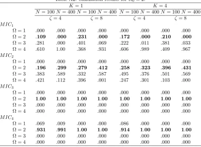
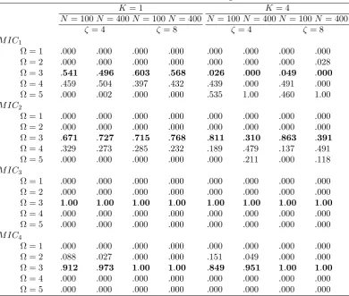
Tables A1-A3 in the appendix report the results of our simulation experiments

in terms of the relative frequency of selecting clusters when the true number

of clusters is 0. The relative frequency of selecting the true number of clusters

is emphasised in bold. Since the property of consistency of b only requires

that f( ) is stricly increasing in and N satis…es limN!1N 1 N = 0 and

limN!1(log logN) 1 N = 1, there is a broad range of values for the penalty

function one can choose from. In this study we set f( ) = such that

M ICj =Nlog

RSS

N T + j forj = 1; :::;4,

where 1 = 2, 2 = logN, 3 = (1= )

h

(logN) 1i and 4 =

p

N. M IC1 and

M IC2 resemble the Akaike and Bayesian information criteria, respectively, except

that they are applied to the clustering selection problem. 3 is motivated from

the fact that (1= )h(logN) 1i _! log logN as _! 0 and hence for any

bounded away from zero, the lower bound of Theorem 2 is satis…ed. As a rule

of thumb, we choose such that 3 lies between 2 and 4, in particular, we set

3 =w 2 + (1 w) 4, w= 1=3. An alternative method of selecting the value of

can be based on the following heuristic algorithm. Firstly, for a given number of clusters a parametric boostrap algorithm is runB times – that is, the responses are

sampled using the optimal partition obtained for this particular cluster number.8

Subsequently, an interval of is determined such that the correct number of

clusters is selected in all bootstrapped samples. After repeating this procedure

times, the intersection of all intervals is chosen as our admissible values. It

is worth noting that in the present study the value of obtained from the rule of

thumb almost always lies in the admissible set of values of . Therefore, in what

follows we report results for this particular 3 value only. It is also possible to

determine using cross-validation, by interpreting this as a smoothing parameter

in a nonparametric regression. For each particular value of = g, evaluated

at a given g, where g = 1; :::; G, the optimal predicted value for yi, by i g ,

is computed by dropping individual i from the sample, estimating the optimal

number of clusters as well as the corresponding partition, and allocating individual

i to the cluster that achieves the lowest prediction error for yi. The optimal

value of is then determined by minimising the objective function, S _g =

Pn

i=1 yi by i g

2

, over a grid of values of : This procedure, however, can

be prohibitively time-consuming for moderately large N and as such we have not

pursued this any further.

As we can see from the tabulated results, both M IC3 and M IC4 perform very

well in all circumstances. This holds true for all values ofN,K and . Naturally,

the performance of both criteria improves with larger values of N and .9 _{On the}

other hand, M IC1 performs poorly in most circumstances in that it constantly

overestimates the true number of clusters. This is not surprising as the criterion is not consistent forN large. In fact, its performance deteriorates as N increases.

M IC2 is a special case of our criterion and performs somewhat better thanM IC1.

Notwithstanding, in a lot of cases it largely overestimates the number of clusters,

especially when 0 = 1;2. We have explored further the underlying reason for

this result. We found that a larger penalty is required in the clustering regression

problem to prevent over-…tting than what is typically used in the standard model selection problem.

Table A4 in the appendix reports the average point estimates of the parameters

for K = 1.10 _{Standard deviations are reported in parentheses.} b

p‘denotes the

pooled estimator that arises by pooling all clusters together, i.e. ignoring

cluster-speci…c heterogeneity in the slope parameters. b_! denotes the estimator of the

parameter vector for the!th _{cluster that arises from the estimated partition when}

0 is estimated usingM IC3. Forbpthe true coe¢cient is taken to be the weighted

average value of the cluster-speci…c unknown slope coe¢cients, with the weights

9 _{does not a¤ect the results when}

0= 1of course.

10_{To save space, we do not report the results obtained forK= 4because similar conclusions}

determined by the size of the true clusters. It is apparent that the bias in b_p is rather large. Its negative sign is due to the fact that the clusters with smaller coe¢cients exhibit relatively larger leverage because the variance of the regressors is larger for these clusters. In contrast, the cluster-speci…c estimators are virtually unbiased even if they are obtained from estimated clusters and the corresponding

estimated partitions. This holds true even forN = 100, although the performance

of the estimators naturally improves as N increases. In conclusion, we see that

the criterion performs well, not only with respect to the estimate of 0, but also

in terms of leading to accurate cluster-speci…c coe¢cients.

6

Empirical Application

We apply the proposed partially heterogeneous framework on a cost function based

on a panel data set of commercial banks operating in the United States. The

issue of how to estimate scale economies and e¢ciency in the banking industry

has attracted considerable attention among researchers due to the signi…cant role that …nancial institutions play in economic prosperity and growth and, as a result, the major implications that these estimates entail for policy making.

6.1

Existing Evidence

In an earlier survey conducted by Berger and Humphrey (1997), the authors report more than 130 studies focusing on the measurement of economies of scale and the

e¢ciency of …nancial institutions in 21 countries. They conclude that while there is lack of agreement among researchers regarding the preferred model with which to estimate e¢ciency and returns to scale, there seems to be a consensus on the fact that the underlying technology is likely to di¤er among banks. To this end,

McAllister and McManus (1993) argue that the estimates of the returns to scale in the banking industry may be largely biased if one applies a single cost function to the whole sample of banks. This result is likely to remain even if one uses a more ‡exible functional form in the data, such as the translog form, because this would

restrict, for example, banks of di¤erent size to share the same symmetric average cost curve. Hence, other interesting possibilities would be precluded, such as ‡at segments in the average cost curve over some ranges, or even di¤erent average cost curves among banks, depending on their size. Thus, the authors conclude:

vary substantially depending on the range of bank sizes included in

the sample. This extreme dependence of the results on the choice

of the sample suggests that there are di¢culties with the statistical techniques employed”, page 389.

Similarly, Kumbhakar and Tsionas (2008) argue that since the banking indus-try contains banks of vastly di¤erent size, the underlying technology is very likely to be di¤erent across banks:

“The distribution of assets across banks is highly skewed. As a result of this, it is very likely that the parameters of the underlying technology

(cost function in this case) will di¤er among banks”, page 591.

Since this view appears to have been widely adopted in the banking literature,

we estimate a partially heterogeneous cost regression model. A conceptually

similar approach has been followed indirectly by Kaparakis et al (1994) and more recently by Kwan (2006), who distinguish between small and large banks and partition the population into two equally-sized sub-samples based on the median

value of total assets. However, this partioning is rather arbitrary and there is no formal justi…cation for imposing two clusters.

6.2

Methodology

The data set consists of a random sample of 551 banks, each observed over a period of 15 years. These data have been collected from the electronic database

maintained by the Federal Deposit Insurance Corporation (FDIC).11

In the theory of banking there is not a univocal approach regarding one’s view

of what banks produce and what purposes they serve. In this paper we follow

the “intermediation” approach, in which the banks are viewed as intermediators

of …nancial and physical resources and produce loans and investments; see also Sealey and Lindley (1977). Under this approach, outputs are measured in money

values and cost …gures include interest expenses. The selection of inputs and

outputs follows closely the study conducted by Hancock (1986). The variables

used in the analysis are: c; the sum of the cost related to the three input prices

that appear below,y1; the sum of industrial, commercial and individual loans, real estate loans and other loans and leases,y2; all other assets,pl; the price of labour,

measured as total expenses on salaries and employee bene…ts, divided by the total

number of employees, pk; the price of capital, measured as expenses on premises

and equipment, divided by the dollar value of premises and equipment, and pf;

the price of loanable funds, measured as total expenses on interest, divided by the dollar value of deposits, federal funds purchased and other borrowed funds.

Hence, the model is speci…ed as follows12_:

c!it = 1!y1;!it+ 2!y2;!it+ 3!pl;!it+ 4!pk;!it+ 5!pf;!it+ !it;

!it = !i+u!it, u!it = r

X

m=1

m

!i mt +"!it. (27)

The assumption of strict exogeneity of the regressors with respect to "!it is

stan-dard in this context; see Kwan (2006), Kumbhakar and Tsionas (2008) and Fries and Taci (2005), among others. However, we deviate from the literature by allow-ing for cross-sectional dependence in the residuals,u!it, by means of a multi-factor

structure. These factors may capture distinct components of time-varying cost

e¢ciency, or common shocks that hit the population of banks at time t. Since

these unobserved common components are likely to be correlated with the regres-sors, strict/weak exogeneity with respect tou!it is violated, leading to biased and

inconsistent parameter estimates.13 We test for error cross-sectional dependence

after estimating(27)allowing for a two-way error components model based on the

…xed e¤ects estimator. We use the test statistics developed by Pesaran (2004)

and Pesaran, Ullah and Yamagata (2008) for this purpose. Both tests soundly

reject the null hypothesis of no error cross-sectional dependence at the 5% level of signi…cance. In particular, Pesaran’s CD statistic equals 26.3 (p-value = 0.000) and the bias-adjusted LM statistic equals 116.9 (p-value = 0.000). Subsequently, we …nd two factors in the residuals based on the eigenvalue ratio test of Ahn and

Horenstein (2008), and accordingly we orthogonalise all variables prior to estima-tion using principal components analysis.

6.3

Main Results

We cluster the sample of banks into up to six clusters based on our partitional

clustering algorithm. The initial partition is chosen on the basis of bank size

using the dynamic programming algorithm analysed in Section 4.2. This algorithm

12_{All variables are expressed in logs.}

13_{A recent literature review on residual factor models is provided by Sara…dis and Wansbeek}

…nds the global minimum for a given number of clusters, i.e. the partition that

minimises the within-cluster sum of squares of the deviations between each cross-sectional unit and the centroid of the cluster in which a particular cross-cross-sectional unit belongs. Bank size is proxied by the …fteen-year average value of total assets for each individual bank.

Table 2 reports the values ofM ICj,j = 1; :::;4, for = 1; :::;6. As we can see,

M IC3 and M IC2 suggest the presence of 5 clusters, whileM IC4, M IC1, suggest

four and six clusters, respectively. These …nding corroborate the results of the

simulation study, which show that under cross-sectional dependence M IC4 might

occasionally underestimate the true number of clusters while the penalty attached

byM IC1 is clearly insu¢cient to prevent over-…tting.

Table 2. Results for estimating the number of clusters.

1 2 3 4 5 6

M IC1 -1086:2 -1227:0 -1249:0 -1260:2 -1270:4 -1271:5

M IC2 -1082:5 -1219:5 -1237:9 -1245:4 -1251:9 -1249:3

M IC3 -1079:6 -1213:8 -1299:2 -1233:9 -1237:4 -1231:9

M IC4 -1072:7 -1200:0 -1208:6 -1209:4 -1203:0 -1190:7

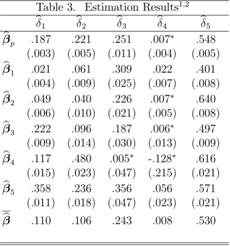
Table 3 reports the estimation results obtained for model (27) for = 5. We

adopt a notation similar to the simulation study; in particular, b_pdenotes the

pooled estimator for the whole sample, b! refers to the …xed e¤ects estimate for

the !th _{cluster and} b _{is the weighted average estimate of all clusters with the}

weights determined by the size of each estimated cluster. The clusters are sorted in ascending order such that cluster 1 contains on average the smallest banks and

cluster 5 the largest banks.

Note that since our clustering procedure minimises the within-cluster residual sum of squares, the properties of the estimated standard errors obtained in the

usual way are no longer known. Therefore, we use bootstrapping to attach a

standard error to the estimated parameters. In particular, for each cluster we draw

a “bootstrap sample” by sampling N times with replacement from the sample.

We then estimate the parameters from the bootstrap sample, and we repeat this

process B(= 200) times, which provides estimates of the distribution one would

get if one were able to draw repeated samples ofN points from the unknown true

distribution.

The results in Table 3 show that there are some large and statistically

example, the estimated coe¢cient of the price of labour, b3, appears to form a

U-shaped function of size, which indicates that in a passage from small to medium sized banks economies of scale increase, and then decrease for large banks. In con-trast, the estimated coe¢cient of loans,b1, appears to rise as bank size increases, although it remains well below one. This implies that while there are increasing

output returns for both small and large banks, the bene…t of small banks getting larger is higher than for banks which are already large. It is worth mentioning

that one draws qualitatively similar conclusions for = 3;4;6, and so the shape

of these pro…les appears to be robust to the choice of clusters. In summary, we see that banks of di¤erent size have di¤erent cost drivers and therefore pooling the data and imposing homogeneity in the slope parameters across the whole sample

may yield misleading results. This becomes apparent when we compare b_p with

b_{, the di¤erence of which is statistically signi…cant for most coe¢cients.}

Table 3. Estimation Results1;2

b₁ b₂ b₃ b₄ b₅ b_p :187 :221 :251 :007 :548

(:003) (:005) (:011) (:004) (:005) b₁ :021 :061 :309 :022 :401

(:004) (:009) (:025) (:007) (:008) b₂ :049 :040 :226 :007 :640

(:006) (:010) (:021) (:005) (:008) b₃ :222 :096 :187 :006 :497

(:009) (:014) (:030) (:013) (:009) b₄ :117 :480 :005 -:128 :616

(:015) (:023) (:047) (:215) (:021) b₅ :358 :236 :356 :056 :571

(:011) (:018) (:047) (:023) (:021) b :110 :106 :243 :008 :530

1:Bootstrapped standard errors in parentheses.

2:‘ ’ denotes non-signi…cance at the 5% level.

7

Concluding Remarks

appears to suggest that while slope parameter homogeneity is usually rejected, the

alternative of allowing these parameters to be individual-speci…c often leads to estimates with large standard errors, counterintuitive sign and inferior forecasting performance. This paper has proposed an intermediate modelling framework that imposes partially heterogeneous restrictions in the slope parameters. The unknown

number of clusters and the corresponding partition are determined based on the concept of ‘partitional clustering’, using an information-based criterion that is strongly consistent for …xed T.

References

[1] Ahn, S. C., Horenstein, A. (2008). Eigenvalue ratio test for the number of factors. Mimeo.

[2] Bai, Z., Rao, C. R., Wu, Y. (1999). Model selection with data-oriented

penalty.Journal of Statistical Planning and Inference 77:103-117.

[3] Baltagi, B. H., Gri¢n, J. M. (1997). Pooled estimators vs. their

heteroge-neous counterparts in the context of dynamic demand for gasoline. Journal

of Econometrics 77:303-327.

[4] Baltagi, B. H, Gri¢n, J. M, Xiong, W. (2000). To pool or not to pool:

homoge-neous versus heterogehomoge-neous estimators applied to cigaretter demand. Review

of Economics and Statistics 82:117-126.

[5] Beasley, J. E, Chu P. C. (1996). A Genetic algorithm for the set covering

problem. European Journal of Operational Research 94:392-404.

[6] Berger, A. N., Humphrey, D. B. (1997). E¢ciency of …nancial institutions:

international survey and directions for future research. European Journal of

Operational Research 98:175-212.

[7] Browning. M., Carro, J. (2007). Heterogeneity and microeconometric

mod-elling. In: Blundell, R., Newey, W., Persson, T. ed. Advances in Economics

and Econometrics 3. Cambridge: Cambridge University Press.

[8] Burnside, C. (1996). Production function regressions, returns to scale, and

[9] Durlauf, S., Johnson, P. (1995). Multiple regimes and cross-country growth

behaviour.Journal of Applied Econometrics 10:365–384.

[10] Everitt, B. (1993).Cluster Analysis. 3rd ed., London: Eward Arnold.

[11] Fernandez-Val, I. (2005). Bias correction in panel data models with individual speci…c parameters. Mimeo.

[12] Fisher, W. D. (1958). On grouping for maximum homogeneity.Journal of the

American Statistical Association 53: 789-798.

[13] Fries, S., Taci, A. (2005). Cost e¢ciency of banks in transition: evidence from

289 banks in 15 post-communist countries. Journal of Banking and Finance

29:55-81.

[14] Gar…nkel, R. S., Nemhauser, G. L. (1969). The set-partitioning problem: set

covering with equality constraints. Operations Research 17:848-856.

[15] Graham, B. S., Powel, J. L. (2008). Identi…cation and estimation of ‘irregular’ correlated random coe¢cient models. Mimeo.

[16] Hancock, D. (1986). A model of …nancial …rm with imperfect asset and deposit

elasticities. Journal of Banking and Finance 10:37-54.

[17] Kapetanios, G. (2006). Cluster analysis of panel datasets using non-standard

optimisation of information criteria.Journal of Economic Dynamics and

Con-trol 30:1389-1408.

[18] Kaparakis, E. I., Miller, S. M., Noulas, A. G. (1994). Short-run cost

ine¢-ciency of commercial banks: a ‡exible frontier approach. Journal of Money,

Credit and Banking 26:875-893.

[19] Kaufman, L., Rousseeuw, P. J. (1990). Finding Groups in Data: An

Intro-duction To Cluster Analysis. New York: John Wiley & Sons.

[20] Kumbhakar, S. C., Tsionas, E.G. (2008). Scale and e¢ciency measurement using a semiparametric stochastic frontier model: evidence from the U.S.

commercial canks. Empirical Economics 34:585-602.

[21] Kwan, S. H. (2006). The X-e¢ciency of commercial banks in Hong Kong.

[22] McAllister, P. H., McManus, D. A. (1993). Resolving the scale e¢ciency

puz-zle in banking.Journal of Banking and Finance 17:389-405.

[23] Pesaran, M. H. (2004). General diagnostic tests for cross section dependence in panels. University of Cambridge, Faculty of Economics, Cambridge Working Papers in Economics No. 0435.

[24] Pesaran, H. M. (2006). Estimation and inference in large heterogeneous panels

With a multifactor error structure. Econometrica 74:967-1012.

[25] Pesaran, H. M., Shin, Y., Smith, R. J. (1999). Pooled mean group

estima-tion of dynamic deterogeneous panels. Journal of the American Statistical

Association 94:621-634.

[26] Pesaran, M. H., Ullah, A., Yamagata, T. (2008). A Bias-adjusted test of error

cross section dependence. The Econometrics Journal 11:105-127.

[27] Rao, M. R. (1971). Cluster Analysis and Mathematical Programming.Journal

of the American Statistical Association 66:622-626.

[28] Rota, G. (1964). The number of partitions of a set. American Mathematical

Monthly 71:498-504.

[29] Sara…dis, V., Wansbeek, T. (2010). Cross-sectional dependence in panel data

analysis. Forthcoming in Econometric Reviews.

[30] Sealey, C. W., Lindley, J. T. (1977). Inputs, outputs, and theory of production

cost at depository …nancial institutions.Journal of Finance 32:1251-1266.

[31] Selim, S. Z., Ismail, M. A. (1984). K-means-type algorithms: a generalized

convergence theorem and characterization of local optimality.IEEE

Transac-tions on Pattern Analysis and Machine Intelligence 6:81-87.

[32] Shao, Q., Wu, Y. (2005). A consistent procedure for determining the

num-ber of clusters in regression clustering. Journal of Statistical Planning and

Inference 135:461-476.

[33] Vahid, F. (1999). Partial pooling: a possible answer to pool or not to pool.

In: Engle, R., White, H., ed. Cointegration, Causality and Forecasting:

[34] Wan, S. J., Wong, S. K. M., Prusinkiewicz, P. (1988). An algorithm for

mul-tidimensional data clustering. ACM Transactions on Mathematical Software

14:153-162.

[35] Yitzhaki, S. (1996). On using linear regressions in welfare economics.Journal

Appendix

A

Proof of Theorem 2

A1. Overparameterised case: 0 < < .

Write

FN (N) FN (N₀)

= Nlog 1 + RSS( ) RSS( 0)

RSS( 0)

+ [f( ) f( 0)] N;

= N RSS( ) RSS( 0) RSS( 0)

+o RSS( ) RSS( 0) RSS( 0)

+ [f( ) f( 0)] N:

We need to show that FN (N) FN (N₀) >0 a.s. for large N. We know

[f( ) f( 0)] > 0 and, under the conditions of the theorem, N grows faster

thanlog logN. Further, asN _{! 1}; RSS( 0)=N is bounded away from 0 and1 almost surely (see, for example, Lemma 2.1 Bai et al. (1999)). Thus the result

follows if we can showRSS( ) RSS( 0) = O(log logN):

We have

RSS( ) RSS( 0)

= T 1

( X

!=1

e

YC ! XeC !b !

2 X0

j=1

e

Y_C0

j XeCj0b0j 2) T 1 ( X !=1 0 X j=1 e

Y_{C !\C}0

j XeC !\Cj0b!jj

2 X0

j=1

e

Y_C0

j XeCj0b0j 2)

= T 1

( X !=1 0 X j=1 e

Y0_C

!\Cj0 I PXe_{C !}\C_j0

e

Y_{C !\C}0

j

0

X

j=1

e

Y_C0 0

j I PXeC_j0

e

Y_C0

j

)

= T 1

( X !=1 0 X j=1

e"0_C

!\Cj0 I PXe_{C !}\C0_j e

"_{C !\C}0

j

0

X

j=1

e"0_C0

j I PXeC_j0 e

"_C0

j

)

= T 1

( ₀ X

j=1

e"0_C0

jPXeC0 j

e

"_C0

j X !=1 0 X j=1 e

"0_{C !\C}0

jPXe_{C !}\C0 j

e

"_{C !\C}0

j

)

= T 1

( ₀ X

j=1

"0_C0

jPXeC0 j

"_C0

j X !=1 0 X j=1

"0_C

!\Cj0PXe_{C !}\C0 j

"_{C !\C}0

j

)

,

(28)

where the last line follows from the idempotent nature of the matrices QC0

j and

QC !\Cj0;

Q0_C0

jPXeC0 j

QC0

j =PXeC0 j

Under the conditions of the theorem, using(19), we have

"0_C

!\Cj0PXe_{C !}\C0 j

"_{C !\C}0

j =O log logN!jj =O(log logN) a.s., (30) whereN!jj = C !\Cj0 . Thus it follows that FN( ) FN ( 0)>0a.s. for N large enough.

A2. Underparameterised case: < 0.

Again we want to show that for N large enough, FN ( ) FN( 0) > 0 a.s.

In this case, (f( ) f( 0)) < 0 and by assumption, limN!1N 1 N = 0. The

result will follow if we show thatNlog (RSS( )=RSS( 0))is positive and of order

N:

The following lemma is necessary for our proof.

Lemma 3 Suppose that Assumption A.4 holds true. Then, for any possible

par-tition with < 0, there exist C ! 2 and C!01; C

0

!2 2 0 such that

C !\C!01 > c0N and C !\C

0

!2 > c0N for any! and N large enough,

(31)

where c0 is a …xed constant.

Proof. See Shao and Wu (2005), Lemma 3.1.

From Lemma 3, for any partition =_fC 1; :::; C g, there exists one cluster

in , say C 1, and two distinct true clusters C0

1 and C20, such that

c0N < C 1\C10 < N and c0N < C 1\C20 < N, (32)

forNlarge enough. Denote the family of subsets C !\Cj0 :j = 1; :::; 0; != 1; :::;

fC 1 \C10; C 1\C20g byL12. Then

RSS( ) RSS( 0)

= T 1 X

!=1

e

YC ! XeC !b !

2 X0

j=1

e

Y_C0

j XeCj0b0j 2!

= T 1 Ye_{C 1\C}0

1 XeC 1\C10b 1

2

+ Ye_{C 1\C}0

2 XeC 1\C20b 1

2

+

T 1

0 @X

L₁₂

e

Y_{C !\C}0

j XeC !\Cj0b !

2 X0

j=1

e

Y_C0

j XeCj0b0j 2

1 A.