Generalized class of synthetic estimators for small areas under systematic sampling scheme

(1)

Generalized class of synthetic estimators

for small areas under systematic

sampling scheme

PANDEY, KRISHAN and Tikkiwal, G.C.

University of Petroleum and Energy Studies, Dehradun, India,

J.N.V.University, Jodhpur, Rajasthan India

15 October 2010

Online at

https://mpra.ub.uni-muenchen.de/37161/

(2)

KRISHAN K. PANDEY1 & G.C.TIKKIWAL2 1

CMES, University of Petroleum & Energy Studies, Dehradun- 248007, India

2

Department of Mathematics & Statistics, J.N.V. University, Jodhpur, Rajasthan -342011, India

ABSTRACT

This paper defines and discusses a generalized class of synthetic estimators for small

domain, using auxiliary information, under systematic sampling scheme. The generalized

class of synthetic estimators, among others, includes the simple, ratio and product synthetic

estimators. Further, it demonstrates the use of the generalized synthetic and ratio synthetic

estimators for estimating crop acreage for small domain and also compares their relative

performance with direct estimators, empirically, through a simulation study.

Key words: Synthetic Estimation; Small Domain; Inspector Land Revenue Circles

(ILRCs); Timely Reporting Scheme (TRS); Absolute Relative Bias (ARB); Simulated

relative standard error (Srse).

1.Introduction

The common feature of small area estimation problem is that when large-scale sample

survey are designed to produce reliable estimates at the national or state level; generally

they do not provide estimates of adequate precision at lower levels like District, Tehsil /

County, and Inspector land Revenue Circle. This is because the sample sizes at the lower

level are generally insufficient to provide reliable estimates using traditional estimators.

Therefore, the need was felt to develop alternative estimators to provide small area statistics

using the data already collected through large-scale surveys. The traditional design based

and alternative estimators are also termed, in the literature of small area estimation,

respectively as direct and indirect estimators.

The indirect estimators are based on methods which increase the effective sample size either

by (i) simulating enough data through appropriate analysis of available data under

appropriate modeling or (ii) by using data from other domains and /or time periods through

models that assume similarities across domain and /or time periods. The only known

method so far belonging to category (i) is SICURE- modeling [TIKKIWAL.(1993)].The

(3)

to category (ii).Among these the synthetic estimators are used for small area estimation,

mainly because of its simplicity, applicability to general sampling design and potential to

increase accuracy in estimation. However, if the implicit model assumption of similarities

across domain and /or time period fails, the synthetic estimator may be badly design biased.

GONZALEZ (1973), GONZALEZ and WAKESBERG (1973), GHANGURDE AND

SINGH (1977, 78), Tikkiwal & Pandey (2007) among others study the synthetic estimator

based on auxiliary variables viz. the ratio synthetic estimator. These studies show that

synthetic estimators provide reliable estimates to some extent.

Tikkiwal and Ghiya (2000) define and discuss a generalized class of synthetic estimators for

small domains, using auxiliary information, under simple random sampling and stratified

random sampling schemes. The generalized class among others includes simple, ratio and

product synthetic estimators. The two authors compare empirically the relative performance

of various direct and synthetic estimators for estimating crop acreage for small domains.

This paper discusses the generalized class of synthetic estimators using auxiliary

information under systematic sampling scheme. The systematic sampling scheme, being

operationally more convenient in practice, is often used in large – scale field surveys under multistage design. In such survey, like crop acreage surveys in India, ultimate stage of

smapling units like villages / households / agricultural fields etc. are selected by systematic

smapling scheme. Systematic sampling scheme, apart from operationally more convinient,

provides more efficient estimators under certain conditions [Cf. Cochran (1977), Sukhatme

et al (1984), Madow (1946) & Osborne, J.G. (1942)].

2. Formulation of the problem & Notations

Let us suppose that we have a finite population U (1,..., ,...,i N) which is divided into

„A‟ non-overlapping small areas U_a of size N_a (a 1,..., )A for which estimates are required. Let the characteristic under study be denoted by „y‟ and also assume that the auxiliary information is availablewhich is denoted by „x‟. Suppose the population units in

small area „a‟ are numbered 1 to Na i.e. Ua (1,...,Na) and na units are to be selected

by systematic sampling scheme. A systematic sample of size n_a is selected from each small

(4)

a

k being an integer) or (ii) by circular systematic sampling scheme, (when N_a n k_a _a). Consequently,

1 A

a a

N N

and

1 A

a a

n n

,

The various population and sample means for characteristic X &Y can be denoted by:

X & Y = Means of the population based on Nobservations.

a

X & Ya= Population means of domain „a‟ based on Naobservations.

ai

x & y_ai= Sample means of domain „a‟ based on n_a observations.

Case (i): For the case Na n ka a i.e. for linear systematic sampling scheme, arrange the

population units into n k_a _a arrays and select a random number, say, i between 1 and k_a then

every kath unit thereafter. So the sample consist na units from Na( n ka a) units, and the

sample is { ,i i k_a,...,i (n_a 1) }.k_a The number i, is called random start and k_a is the sampling interval. Further, let x_{a i j} & y_{a i j} denote the values of the auxiliary variate and characteristic under study respectively for the jth unit of the ith sample bearing serial number

i +(j-1) k_a , i =1,..., k_a ; j =1,..., n_a . Therefore,

1

a ai j

i j

a

X x

N , . ₁

1 na

ai ai j

j a

x x

n ,

1

a ai j

i j

a

Y y

N and . ₁

1 na

ai ai j

j a

y y

n

Various mean squares and coefficient of variations of subpopulation „U_a‟ for auxiliary variate x & characteristic under study, y is denoted by

2 _. 2

1 1 ( ) 1 a a k

x ai a

i a

S x X

k ,

a a x x a S C

X and

2 2 . 1 1 ( ) 1 a a k

y ai a

i a

S y Y

k , a a y y a S C Y

The coefficient of covariance between X and Y is denoted by

a a a a x y x y a a S C

X Y , where ₁ . .

1 ( )( ) 1 a a a k

x y ai a ai a

i a

S y Y x X

k

(5)

sampling design. Here in this case a random number is chosen from 1 to N_a and the units

corresponding to this random number are chosen as the random start. There after every k_ath

unit is chosen in a cyclic manner till a sample of na units is selected. Thus if i is a number

selected at random from 1 to N_a, the sample consists of units corresponding to these numbers are

{i (j 1) }k_a if i (j 1)k_a N_a

{i (j 1)ka Na} if i (j 1)ka Na , j =1,2,…….., na

In this case the x_{a i j} & y_{a i j} denote the values of the auxiliary variate and characteristic

under study respectively for the jth unit of the ith sample bearing the number {i (j 1) }k_a

or {i (j 1)k_a N_a} as the case may be for j 1, 2,...,n_a.The various mean squares and

coefficient of variations of sub population „Ua‟ for auxiliary variate x & characteristic

under study, y in this case will be as follows:

2 2 1 . 1 1 ( ) 1 a a N

x ai a

i a

S x X

N ,

2 1 2 1 2 a a x x a S C

X and

2 2 1 . 1 1 ( ) 1 a a N

y ai a

i a

S y Y

N ,

2 1 2 1 2 a a y y a S C Y

The coefficient of covariance between X and Y is denoted by

₁ 1a a

a a x y x y a a S C

X Y , where

2 2

1 . .

1 1 ( ) ( ) 1 a a a N

x y ai a ai a

i a

S y Y x X

N

3. Generalized Class of Synthetic Estimators

Following Srivastava (1967), we, in this section, define a generalized class of synthetic

estimators of population mean Y_a based on the auxiliary variable „x‟ under Systematic Sampling Scheme as follows.

,

w

s a w

a

x y y

X

... (3.1)

Where β is a suitably chosen constant , and

' ''

. .

' ''

. .

w a ai a ai

y p y p y x p x p x

(6)

Where ' denotes the summation over those small areas where N_a n k_a _a

and '' denotes summation over those small areas where N_a n k_a _a and

a a

N p

N . Here clearly

( _w)

E y Y and E x( _w) X ... (3.3)

The above estimator ys a, perform well under the following condition

Ya Xa Y X( )

... (3.4)

It is noted that the synthetic estimator ys a, is consistent; if the condition given in (3.4) is

satisfied.

Remark 3.1

If β = 0, -1, 1, the estimator y_{s a}_, in (3.1) reduces to y_{s s a}_{, ,} y_w , _{, ,} w

s r a a

w

y

y X

x , and

, ,

w

s p a w

a

x

y y

X respectively with synthetic condition Ya Y ,

a

Y Y

X X , and

( )

a a

Y X Y X .

4. Design Bias and Mean Square Error of Generalized Synthetic Estimator

Design Bias and Mean Square Error of generalized synthetic estimator, under the synthetic

condition given in (3.4), is as follows

' 2 '' 2 1

,

1 ( 1)

( ) a y xa a a x ya a

s a a _a a _a a

a a

S S

k N

B y Y p p

k X Y N X Y

2 2

' 2 '' 2 1

2 2

1 ( 1)

( 1)

2

a a

x x

a a

S S

k N

p p

k X N X ... (4.1)

(7)

2 2

' '' 1

2 2 2 2

, , 2 2

1 ( 1)

( ) ( ) a ya a ya

s a s a a a _a a _a a

a a

S S

k N

MSE y E y Y Y p p

k Y N Y

2 2

' 2 '' 2 1

2 2

1 ( 1)

(2 1) a xa a xa

a a a a a a S S k N p p

k X N X

4 ' 2 a 1 y xa a '' 2 ( a 1) 1x ya a

a a a a a a S S k N p p

k X Y N X Y

2 2 ' 2 a 1 y xa a '' 2( a 1) 1y xa a

a a a a a

a a

S S

k N

Y p p

k X Y N X Y

2 2

' 2 '' 2 1

2 2

1 ( 1)

( 1) 2 a a x x a a a a a a a a S S k N p p

k X N X ... (4.2)

The suitable value of β is the one for which MSE y( s a, )is minimum. So minimizing the

,

( _{s a})

MSE y with respect to β under synthetic condition, gives simplified expression for β, if

a

X X as follows

' 2 '' 2 1

2 2

' 2 '' 2 1

2 2

1 ( 1)

a a a a

a a

y x x y

a a a a a a a a x x a a a a a a a a S S k N p p

k X Y N X Y

S S

k N

p p

k X N X

... (4.3)

It is noted that the expression of MSE for direct estimator under linear & circular systematic

sampling design, is minimum if a a₂

a x y

x

C

[Cf. Srivastava (1967)].

5. Estimation of Mean square errors

Since a systematic sample can be regarded as a random selection of one cluster, it is not

possible to give an unbiased or even consistent estimator of the design variances of

. ai

(8)

formulae. Unfortunately, if followed indiscriminately this practice can lead to badly biased

estimators and incorrect inferences concerning the population parameters of interest.

Wolter (1984, 1985) investigate several biased estimators of variances with a goal of

providing some guidance about when a given estimator may be more appropriate than other

estimators. The criterion to judge the various estimators on the basis of their bias, their

mean square error, and proportion of confidence interval formed using the variance

estimators which contain the true population parameter of interest. This study suggests the

use of biased but simple estimator v2y for V y( ai.), when sample size is very small for both

the situations viz., when Na n ka a and Na n ka a. The expression of v2y is given as

follows;

2

1 (1

)

2(

1)

a

n

i j y

j

a a

a

v

f

n

… (5.1)

, 1

i j i j i j i j

a

where

a

y

n

and

f

N

… (5.2)

Similarly estimate of V x( ai.)is given by v2x, where

2

1 (1

)

2(

1)

a

n

i j x

j

a a

b

v

f

n

… (5.3)

, 1

i j i j i j i j

a

where

b

x

n

and

f

N

… (5.4)

We note that above estimators v₂_y and v₂_x are based on overlapping differences of y_{i j}

& xi j respectively. Further, the estimate of covariance term between yai. and xai., given by

Swain (1964), is

. . 2 2

ˆ

(

_ai

,

_ai

)

_y _x

Cov y

x

r v v

… (5.5)

Where r is correlation coefficient between x and y observations based on the sample of size

a

(9)

5.1 Estimation of mean square error of direct estimator

Following Srivastava (1967), the generalized class of direct estimators of Y_a under

systematic sampling scheme is .

, .

G ai

d a ai

a

x y y

X

.

Its mean square under case (i) is

2 . . . .

, 2 2

( ) ( ) 2 ( , )

( G ) ai ai ai ai

d a a

a a a a

V y V x Cov y x

MSE y Y

Y X X Y

or ( , ) ( .) 2 2 ( .) 2 ( ., .)

G

d a ai a ai a ai ai

MSE y V y R V x R Cov y x … (5.6)

where a

a a

Y R

X , Thus a consistent estimator of ( , )

G d a

MSE y is given by

2 2

, 2 2 2 2

(

_{d a}g

)

_y _a _x

2

_a _y _x

mse y

v

r v

r r v v

… (5.7)

Where a a

a

y

r

x

is the ratio of sample means. It is also observed that the mean square error

for direct estimator in case of circular systematic sampling is given

by , 2 2. 2 2. . .

( ) ( ) ( , )

2

G ai c ai c ai ai c

d a _c a

a a a a

V y V x Cov y x

MSE y Y

Y X X Y

2 2

, ( .) ( .) 2 ( ., .)

G

d a _c ai c a ai c a ai ai c

MSE y V y R V x R Cov y x … (5.8)

Thus consistent estimator of _{d a}G_,

c

MSE y is given by

' 2 2 ' ' '

, 2 2 2 2

( _{d a}g )_c _y _a _x 2 _a _y _x

mse y v r v r r v v _{… (5.9}₎

Where v₂'_y and v2'x are the estimates of variances of V y( ai.)c and V x( ai.)c respectively in

case of circular systematic sampling design. To be calculate similarly as of v₂_x and v₂_y.

5.2Estimation of mean square error of synthetic estimator

The expression for the Mean Square Error given in (4.2), can be approximated under the

(10)

' ₂ ' ' ₂ ₂ ₂ ' ₂ ' ' ₂

, . . . .

( _{s a}) _a ( _ai) _a ( _ai)_c _a _a ( _ai) _a ( _ai)_c

a a a a

MSE y p V y p V y R p V x p V x

2 _a ' _a2 ( _ai_., _ai_.) ' ' _a2 ( _ai_., _ai_.)_c

a a

R p Cov y x p Cov y x … (5.10)

Thus a consistent estimator of MSE y( _{s a}_, ) is given by

' ₂ ' ' ₂ _' ₂ ₂ ' ₂ ' ' ₂ _'

, 2 2 2 2

( _{s a}) _a _y _a _y _a _a _x _a _x

a a a a

mse y p v p v r p v p v

' ₂ '' ₂ _' _'

2 2 2 2

2 _a _a _y _x _a _y _x

a a

r p r v v p r v v _{… (5.11}₎

Where a a

a

y

r

x

is the ratio of sample means.

6.Crop Acreage Estimation for Small Domain- A Simulation Study

T

his section demonstrates the use of the generalized synthetic and ratio synthetic

estimators to obtain crop acreage estimates for small domain and also compare their relative

performance with the corresponding direct estimators empirically, through a simulation

study. This is done by taking up the state of Rajasthan, one of the states in India, for case

study [Cf. Tikkiwal & Ghiya (2000)].

6.1 Existing methodology for estimation

In order to improve timelines and quality of crop acreage statistics, Timely Reporting

Scheme (TRS) is used by most of the States of India. The TRS has the objective of

providing quick and reliable estimates of crop acreage statistics and there-by production of

the principle crops (i.e. Jowar, Bajra,Maize etc.) during each agricultural season. Under the

scheme, the Patwari (Village Accountant) is required to collect acreage statistics on a

priority basis in a 20 percent sample of villages, selected by stratified linear systematic

sampling design taking Tehsil (a sub-division of the District) as a stratum. These statistics

are further used to provide state level estimates using direct estimators viz. unbiased (based

on sample mean) and ratio estimators.

6.2 Details of the simulation study

For collection of revenue and administrative purposes, the State of Rajasthan, like most of

(11)

divided into a number of Tehsils and each Tehsil is also divided into a number of Inspector

Land Revenue Circles (ILRCs). Each ILRC consists of a number of villages. For the present

study, we take ILRCs as small domains.

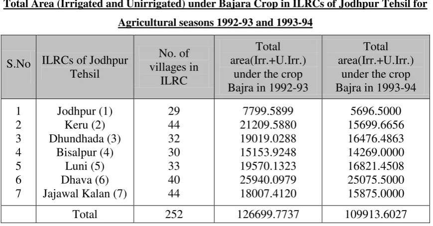
In the simulation study, we undertake the problem of crop acreage estimation for all

Inspector Land Revenue Circles (ILRCs) of Jodhpur Tehsil of Rajasthan. They are seven in

number and these ILRCs contain respectively 29, 44, 32, 30, 33, 40 and 44 villages. These

ILRCs are small domains from the TRS point of view. The crop under consideration is

Bajra (Indian corn or millet) for the agriculture season 1993-94. The Bajra crop acreage for

agriculture season 1992-93 is taken as the auxiliary characteristic x. The various

[image:11.595.85.520.328.555.2]

information regarding the ILRCs of Jodhpur Tehsil are provided in the Table 6.2.1.

Table 6.2.1

Total Area (Irrigated and Unirrigated) under Bajara Crop in ILRCs of Jodhpur Tehsil for Agricultural seasons 1992-93 and 1993-94

S.No ILRCs of Jodhpur Tehsil

No. of villages in

ILRC

Total area(Irr.+U.Irr.)

under the crop Bajra in 1992-93

Total area(Irr.+U.Irr.)

under the crop Bajra in 1993-94

1 2 3 4 5 6 7

Jodhpur (1) Keru (2) Dhundhada (3)

Bisalpur (4) Luni (5) Dhava (6) Jajawal Kalan (7)

29 44 32 30 33 40 44

7799.5899 21209.5880 19019.0288 15153.9248 19570.1323 25940.0979 18007.4120

5696.5000 15699.6656 16476.4863 14269.0000 16821.4508 25075.5000 15875.0000

Total 252 126699.7737 109913.6027

Below the list of all those estimators, whose relative performance is to be assessed for

estimating population total T_a of small domain for „a‟ = 1, 2 …7.

Direct estimators

Direct ratio estimator .

1, , ,

.

ˆ ai

a a d r a a a

ai

y

T N y N X

x

Direct general estimator .

2, , .

ˆ G ai

a a d a a ai

a

x T N y N y

(12)

Where _.

1

1 na

ai ai j

j a

y y

n ; and . ₁

1 na

ai ai j

j a

x x

n

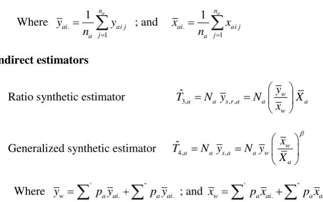
Indirect estimators

Ratio synthetic estimator ˆ_3, _{, ,} w

a a s r a a a

w

y

T N y N X

x

Generalized synthetic estimator ˆ_4, _, w

a a s a a w

a

x T N y N y

X

Where y_w ' p y_a _ai_. " p y_a _ai_. ; and x_w ' p x_a _ai_. " p x_a _ai_.

Before simulation, we examine the condition of generalized synthetic and synthetic ratio

estimators as given in Eq. (3.4) and in remark (3.1). These results are presented in following

tables 6.2.2 & 6.2.3 respectively. We note that both the above conditions meet for ILRCs

[image:12.595.92.423.74.281.2]

(3), (5), (7) deviate moderality for ILRCs (4) & (6) and deviate considerably for ILRC (7).

TABLE 6.2.2

Absolute Differences (Relative) under Synthetic Assumption of Synthetic Ratio Estimator for Various ILRCs.

ILRC _/

a a

Y X Y /X ₍ _/ ₎ ₍ _/ ₎ _/ ₁₀₀

a a a a

Y X Y X Y X

(1)

(2)

(3)

(4)

(5)

(6)

(7)

0.73036

0.7402

0.8663

0.9416

0.8595

0.9666

0.8815

0.86751

18.17

17.19

0.13

7.86

0.91

10.25

(13)

[image:13.595.109.496.117.336.2]

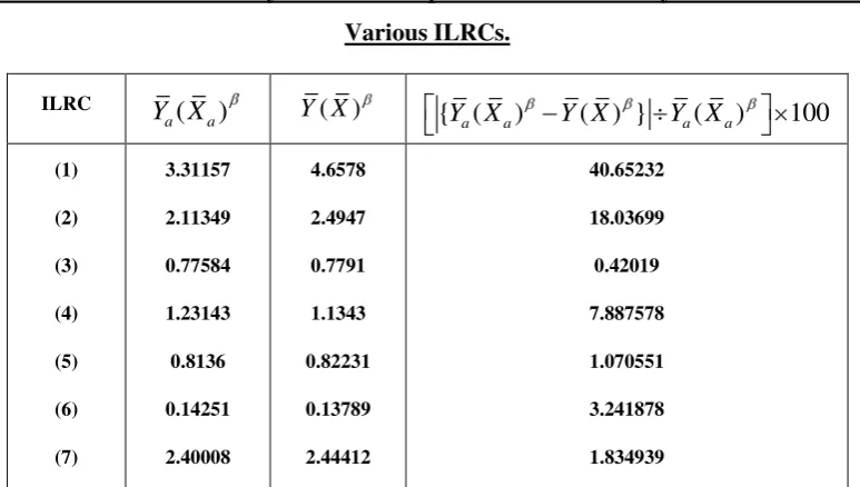
TABLE 6.2.3

Absolute Differences under Synthetic Assumption of Generalized Synthetic Estimator for Various ILRCs.

ILRC ₍ ₎

a a

Y X Y X( ) _{{ (} ₎ _{( ) }} ₍ ₎ ₁₀₀

a a a a

Y X Y X Y X

(1) (2) (3) (4) (5) (6) (7) 3.31157 2.11349 0.77584 1.23143 0.8136 0.14251 2.40008 4.6578 2.4947 0.7791 1.1343 0.82231 0.13789 2.44412 40.65232 18.03699 0.42019 7.887578 1.070551 3.241878 1.834939

Now for simulation study, taking villages as sampling units, 500 independent systematic

samples each of size 25, 50, 63, 76 and 88 are selected by the procedure described in section

2 from the population of 252 villages of Jodhpur Tehsil. The simulation length was

estimated with the help of concept discussed by Whitt, W. (1989) & Murphy, K.E. Carter,

C.M. & Wolfe, L. H. (2001), based on the steady state condition.

That is selecting approximately 10 percent, 20 percent, 25 percent, 30 percent and 35

percent villages independly form each ILRC. For each small area estimator under

consideration and for each sample size we compute Absolute Relative Bias (ARB) and

Average Square Error (ASE), as defined below.

500 , 1 , 1 _ˆ 500 ˆ

( ) 100

s

k a a

s k a

a

T T ARB T

T ... (6.1)

and , ,

,

ˆ

( )

ˆ

( ) _ˆ 100

( ) k a k a k a ASE T Srse T

E T ... (6.2)

Where 500 ₂ , , 1 1 ˆ ˆ ( ) 500 s

k a k a a

s

ASE T T T and

500 , , 1 1 ˆ ˆ ( ) 500 s

k a k a

s

E T T

(14)

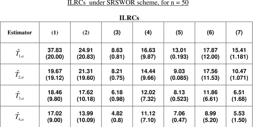
6.3 Results

We present the results of ARB and Srse in Table (6.3.1) only for n 50, (a sample of 20

present villages, as presently adopted in TRS) as the findings from other tables are similar.

For assessing the relative performance of the various estimators, we have to adopt some rule

of thumb. Here we adopt the rule that at the ILRCs level, an estimator should not have Srse

more than 10 % and bias more than 5%.

We note from the table that none of the estimators satisfy the rule in ILRCs 1 and 2. This

may be because, in these circles, there is considerable deviation from the synthetic

condition, as observed earlier. In ILRCs 4 and 6, where the condition deviate moderately,

4,

ˆ _a

T alone satisfies the rule to some extent. In ILRCs 3, 5 and 7, where the synthetic

condition closely meet, both Tˆ_3,_a and Tˆ_4,_a satisfy the rule but Tˆ_4,_a‟s performance is slightly

[image:14.595.103.542.316.537.2]

better than Tˆ_3,_a.

Table 6.3.1

Simulated relative standard error (in %) and Absolute Relative Bias (in %) for various

ILRCs under SRSWOR scheme, for n = 50

ILRCs

Estimator (1) (2) (3) (4) (5) (6) (7)

1,

ˆ_a

T _(20.00)37.83 _(20.83)24.91 _(0.81)8.63 16.63 _(9.87) _(0.193)13.01 _(12.00)17.87 _(1.181)15.41

2,

ˆ

a

T _(19.12)19.67 _(19.60)21.31 _(0.75)8.21 14.44 _(9.66) _(0.085)9.03 _(11.53)17.56 _(1.071)10.47

3,

ˆ

a

T 18.46 _(9.80) _(10.18)17.62 _(0.98)6.18 12.02 _(7.32) _(0.523)8.13 11.86 _(6.61) _(1.68)6.51

4,

ˆ

a

T 17.02 _(9.00) _(10.09)13.99 _(0.8)4.82 11.12 _(7.10) _(0.47)7.06 _(5.20)8.99 _(1.50)5.53

(15)

From the above analysis it is clear that if the synthetic estimators do not deviate

considerably from their corresponding synthetic condition then, performance of the

synthetic estimators Tˆ_3,_a and Tˆ_4,_a, based on a sample of 20 present villages ( as presently

being taken under TRS), is satisfactory at the level of ILRCs. Therefore, these estimators

are also likely to perform better both at Tehsil and district levels. When the synthetic

estimators deviate considerably from their corresponding synthetic condition then we

should look for other types of estimators such as those obtained through the SICURE MODEL_[_TIKKIWAL_{, B.D. (1993)] and assess their relative performance through studies of}

the kind, in series, over some years for crop acreage estimation.

ACKNOWLEDGEMENT:

The author is very thankful to the referee for his valuable suggestions.

REFERENCES

Ghangurde, P.D. and Singh, M.P. (1978).“Evaluation of efficiency of synthetic estimates”, Proceeding of the Social Statistical Section of the American Statistical Association, 53-61.

Cochran, W.G. (1977).“Sampling Techniques”,Wiley & Sons.

Gonzalez, M.E. (1973). “Use and evaluation of synthetic estimates”, Proceedings of the social statistical section of American Statistical Association, 33-36.

Gonzalez, M. E. and Waksberg, J. (1973).“Estimation of the error of synthetic estimates”, paper presented at first meeting of the International association of survey

statisticians, Vienna, Austria, 18-25, august 1973.

Lahiri, D.B. (1954).“On the question of bias of systematic sampling”, Proceedings of the world Population Conference, 6, 349-62.

Murphy, K.E. Carter, C.M. & Wolfe, L.H. (2001) “How long should I simulate, and for how many trials?A practical guide to reliability simulations”,Reliability and

Maintainability Symposium, 2001, Proceedings, Philadelphia, p.p. 207-212.

(16)

Osborne, J.G. (1942).“Sampling errors of systematic & random survey of covertype areas”, Journal of American Statistical Association 37:256-264.

Srivastava, S.K. (1967). “An estimator using auxiliary information in sample surveys”, Calcutta Statist. Assoc. Bull. , 121-132.

Swain, A.K.P.C. (1964).“The use of systematic sampling in ratio estimates”, JISA, 2, 160-164.

Sukhatme, P. V. Sukhatme, B. V., Sukhatme, S. and Asok, C. (1984). “Sampling Theory of Surveys with Applications (3rd Edition)”, Indian Society of Agricultural

Statistics, New Delhi.

Tikkiwal, G.C. and Ghiya, A. (2000). “A generalized class of synthetic estimators with application of crop acreage estimation for small domains”, Biom, J, 42, 7,

865-876.

Tikkiwal, B.D. (1993). “Modelling through survey data for small domains”,

Proceedings of International Scientific conference on small area statistics and survey

Design (held in September, 1992 at Warsaw, Poland).

Tikkiwal, G.C. and Pandey, K.K. (2007).“On Synthetic and Composite Estimators for Small Area Estimation under Lahiri – Midzuno Sampling Scheme”, Statistics in

Transition New Series, vol. 8. No. 1, 111-123.

Wolter, K.M. (1984, 1985).“An investigation of some estimators of variances for systematic sampling”, J. Amer. Stat. Assoc., 79, 781-90.