Design of a High Resolution Time-of-Flight Crystal Analyser Spectrometer
and
Hydrogen Diffusion in Intermetallic Compounds.
by
Stuart Ian Campbell
A thesis submitted in partial fulfilment of the requirements of the Degree of
Doctor of Philosophy
Contents
1. Introduction... 1
1.1 Neutron properties and condensed matter research... 1
1.2 Production of Neutrons ... 1
1.2.1 High Flux Reactor (HFR) at the ILL ... 2
1.2.2 Pulsed Spallation Source, ISIS ... 3
1.3 Laves Phase Intermetallic Compounds ... 7
2. Neutron Scattering Theory ... 11
2.1 Neutron scattering length ... 11
2.2 Coherent and incoherent scattering ... 13
2.3 Neutron optics ... 14
2.3.1 Refractive index... 14
2.3.2 The representation of scattering density by a virtual potential . 16 2.3.3 Mirror reflection ... 19
2.4 Quasi-elastic neutron scattering ... 20
2.4.1 Jump diffusion ... 22
2.4.2 The Chudley-Elliott model ... 23
2.4.3 Jump diffusion on non-Bravais lattices ... 26
3. Neutron Instrumentation ... 31
3.1 Introduction ... 31
3.2 Detection of neutrons ... 31
3.2.1 The He3gas detector... 32
3.2.2 The zinc sulphide detector ... 32
3.3 Neutron transport... 33
3.3.1 Supermirrors ... 33
3.3.2 Neutron guides... 34
3.3.2.1 Converging guides ... 36
3.4 Polarised neutrons ... 37
3.4.1 Polarising benders... 37
3.4.2 He3 filter... 39
3.4.3 Spin flippers... 39
3.5 Neutron energy selection ... 40
3.5.1 Monochromators and analysers ... 40
3.5.2 Thermal diffuse scattering and effect of cooling analysers ... 41
3.5.3 Choppers ... 43
3.6 Neutron Instruments ... 44
3.6.1 The high resolution inelastic spectrometer, IRIS... 44
3.6.2 The IN10 high resolution backscattering spectrometer ... 47
3.6.3 The diffuse scattering spectrometer, D7 with polarisation analysis... 49
3.6.4 Time-focused crystal analyser spectrometer, TFXA ... 50
3.6.5 The MuSR muon spectrometer at ISIS ... 51
4. The Design & Simulation of the OSIRIS Spectrometer ... 52
4.1 Introduction ... 52
4.2 Overview of the OSIRIS Project ... 52
4.3 History of the Monte Carlo technique ... 53
4.4 Basic design considerations... 54
4.5 Description of the program... 55
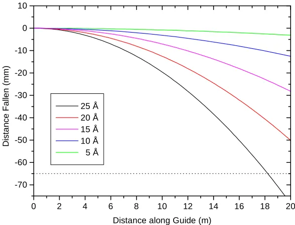
4.5.1 Effect of gravity... 58
4.5.2 Moderator energy structure... 59
4.5.3 Model used for moderator time distribution... 59
4.6 Results of guide simulations... 61
4.6.1 Effect of altering the coating of the converging guide ... 64
4.6.2 The impact of the “m”-value with guide length ... 65
4.6.3 Improvements to the IRIS guide ... 67
4.6.4 Effect of missing section in shutter guide... 69
4.8 Microguide Testing Device, MITED... 75
4.8.1 The microguide technique ... 75
4.8.2 Experimental setup and results ... 77
4.9 Reflectivity of coated stainless steel... 80
4.10 Surface roughness measurements... 80
4.11 Why do we need to understand resolution functions?... 85
4.12 Energy resolution... 85
4.13 Analyser geometry... 86
4.14 Resolution considerations ... 88
4.15 Possible designs for the analyser bank ... 91
4.15.1 Extending the IRIS analyser bank ... 92
4.15.2 Expected performance of OSIRIS ... 94
4.16 Conclusion... 98
5. C-15 Laves Phase Compounds... 100
5.1 Introduction ... 100
5.2 Choice of samples ... 100
5.3 Sample preparation... 101
5.4 X-ray and neutron diffraction ... 101
5.5 Quasi-elastic neutron scattering measurements... 108
5.5.1 Experimental procedure... 108
5.5.2 Analysis procedure ... 109
5.5.3 TiCr1.85H0.43Results ... 110
5.5.4 HfV2H0.3Results... 116
5.5.5 Discussion... 119
5.6 Muon Spectroscopy... 123
5.6.1 Muon production ... 123
5.6.2 Experimental procedure and analysis ... 124
5.6.3 ZrTi2Hx(x=3.6,5.4) Results and discussion ... 126
5.6.4 HfV2H0.15Results and discussion... 132
5.7 Inelastic neutron scattering measurements of TiCr1.85H0.43... 134
6. Conclusion and Final Remarks ... 138
6.1 Summary of OSIRIS... 138
6.2 C-15 Laves Phase Compounds... 139
Publications ... 141
Appendix I ... 144
Appendix II... 145
Appendix III ... 151
List of Tables
1.1 Atoms and common interstitial sites for a AB2type C-15 ... compound ... 9 2.1 The scattering cross sections for a number of nuclei that are
commonly found in C-15 laves phase metal hydride systems ... 14 3.1 Characteristics of the IRIS analyser arrays ... 46 3.2 Characteristics of the IN10 spectrometer for different
monochromator and analyser configurations... 48 4.1 Detailed OSIRIS guide parameters... 62 4.2 Detailed IRIS guide parameters ... 63 4.3 R.M.S. roughness values obtained for various supermirror
samples ... 82 4.4 Co-ordinates and orientations of the graphite analyser crystals for
the proposed IRIS upgrade. The values stated are for a vertical section through the sample tank at a scattering angle of 90°. Also shown are the orientation angles required to focus the neutrons
onto the detector. ... 93 4.5 Values of the vertical distance to the detector for a given
backscattering angle... 94 4.6 Positions and orientations for two possible configurations of the
OSIRIS analyser bank. . Also shown are the orientation angles
required to focus the neutrons onto the detector... 97 5.1 Effect on the tetrahedral interstitial sites of a C-15 Laves structure
of substituting a B-type atom with an A-type atom ... 100 5.2 Summary of the lattice parameter obtained from XRD
measurements on the various samples used... 102 5.3 Values for Dtobtained from a linear fit to the low-Q region of the
HWHM against Q2curve for TiCr1.85Hx... 112 5.4 Parameters obtained from simultaneous fits to the polycrystalline
5.5 Values obtained for Dtfrom fitting the low-Q data... 117 5.6 Properties of the proton and positive muon... 123 5.7 Values for the instrumental asymmetry,α... 125 5.8 Activation energies obtained from high temperature region of
Figure 5.24 and Figure 5.26... 130 5.9 Basic description of peak centres and areas for each of the
List of Figures
1.1 Production of neutrons by nuclear fission ... 2 1.2 A vertical view of the ILL High Flux Reactor... 3 1.3 Neutron production process at a pulsed spallation source... 4 1.4 A Plan view of the ISIS Pulsed Neutron Source, showing its main
components, the linear accelerator, synchrotron, target station and suite of instruments... 5 1.5 The predicted 4πequivalent fluxes for three ISIS moderators
compared with the fluxes of the three moderators at the ILL (Taylor 1984). The designation AP refers to the asymmetric
poisoned ambient water moderator... 6 1.6 The C-15 Laves phase structure, illustrating the different types of
interstitial site. The A atoms are the larger blue spheres, and the B are the smaller red spheres. Also shown are the b, e and g
tetrahedral interstitial sites (grey spheres) ... 8 2.1 Geometry for a neutron scattering experiment ... 11 2.2 Geometrical convention used for neutron wave being scattered in
a given direction ... 15 2.3 Neutron optical behaviour at an interface between media 1 and 2;
(a) refraction, (b) critical glancing angle, and (c) total reflection
(taken from Williams, 1988) ... 20 3.1 A schematic sketch of how the reflectivity of a surface compares
for a (i) monolayer reflective surface, (ii) a multilayer of constant thickness and (iii) a supermirror ... 34 3.2 Definition of the line of sight, Loand characteristic angleγ*for a
circularly curved guide ... 35 3.3 A schematic representation of a polarising bender... 38 3.4 A cross sectional view of a polarising supermirror bender as used
section 2.3.2. ... 38 3.5 Measured neutron polarisation and transmission for an ILL He3
filter. The dotted curve represents the neutron polarisation
corrected for losses in the magnetic shielding (Kulda et al. 1998).... 39 3.6 Single crystal of pyrolitic graphite diffraction pattern shown as
a function of offset angle from the Bragg condition (Carlile et
al., 1994) ... 42 3.7 Scattering patterns from pyrolitic graphite showing the reduction
in intensity of the phonon peaks with fall in temperature (Carlile et al., 1994) ... 43 3.8 A neutron disc chopper... 44 3.9 The IRIS high-resolution spectrometer at the ISIS pulsed neutron
source... 45 3.10 The primary flight path of the IRIS spectrometer (taken from
Carlile and Adams; 1992)... 46 3.11 Layout of the IN10 back-scattering spectrometer at the ILL. ... 48 3.12 Schematic diagram of the diffuse scattering instrument D7 at the
ILL, Grenoble. (a) Be filter or polarizer; (b) main monitor; (c) slit system; (d) flipper and second polarizer for psueudostatistical chopper; (e) disc chopper or flipper; (f) detector banks 1-3 with supermirror polarizing Sollers; (g) vertical detector bank 4; (h)
sample, (taken from Bank and Maier, 1988) ... 49 3.13 The TFXA crystal analyser spectrometer at the ISIS Facility... 50 3.14 The MuSR muon spectrometer situated at the ISIS Facility... 51 4.1 A schematic diagram of the OSIRIS spectrometer and
diffractometer ... 53 4.2 Reflectivity curve for a “m” = 4 supermirror (used in simulation) ... 57 4.3 Measured reflectivity profile for neutrons of up (∆) and down (τ)
spin states for a “m” = 2 polarising Co/Ti supermirror
of the OSIRIS guide, assuming that it had entered the guide at the very top and only has a horizontal velocity component... 58 4.5 The experimental and fitted moderator shapes as measured
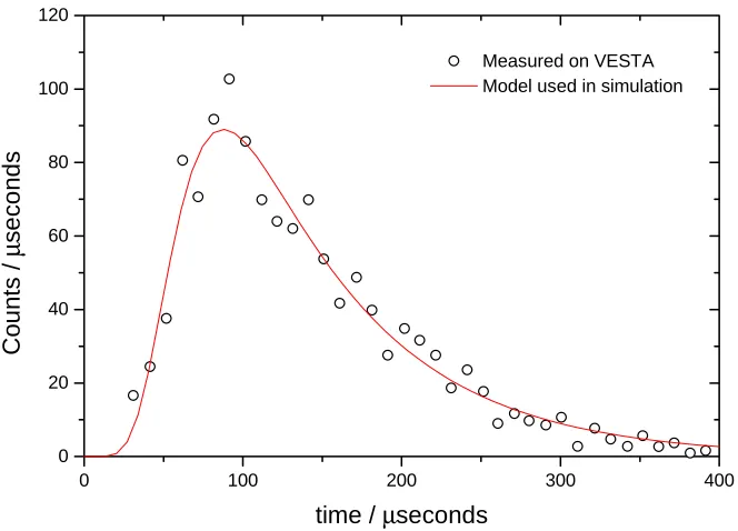
on CRISP (Martín, 1996)... 59 4.6 Time structure of the neutron pulse emanating from the 25 K
ISIS moderator for a wavelength of 6.28 Å. The data points are measured values from VESTA (Carlile, 1996) and the solid line is the model used in the Monte Carlo simulations (equation 4.2). .... 60 4.7 Comparison between measured intensity and Monte Carlo
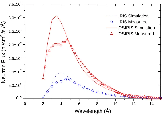
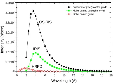
simulations for the IRIS spectrometer ... 62 4.8 The neutron intensity of HRPD, IRIS and OSIRIS as a function of
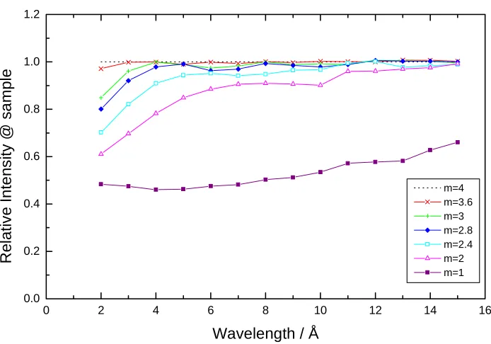
wavelength. The HRPD results are measured intensities. IRIS and OSIRIS results are Monte Carlo simulations... 63 4.9 Intensities for different converging guide coatings relative to the
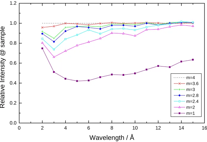
intensity observed with a m = 4 supermirror ... 64 4.10 Relative intensities for different converging guide coatings to the
intensity observed with a m = 4 supermirror. A bender is also
present in the incident beam. ... 65 4.11 Ratio of the increase in intensity for different guide coatings over
that m = 1 case as a function of the neutron wavelength and the
length of the guide. ... 66 4.12 A cut through the surface shown in Figure 4.11 for discrete values
of the guide length ... 67 4.13 The simulated increase in flux of IRIS as a result of closing missing
sections of the guide (installed during the OSIRIS construction)... 68 4.14 The intensity gain factor for the IRIS guide if we replace the
existing nickel guide with a supermirror coated one ... 69 4.15 The reduction in intensity as a result of having a gap on one side of
the OSIRIS shutter guide section. The red solid line is a linear fit to the data which has a gradient of -0.347±0.033. ... 70 4.16 Beam asymmetry at the guide exit as a function of different surface
which exit on the convex ... 71 4.17 Comparison of theoretical and simulated transmission for curved
supermirror guides with nickel (m = 1) and supermirror (m = 2) coatings ... 72 4.18 Theoretical and simulated transmission for a lossy curved guide.
The reflectivity of the surfaces was fixed at R=0.92 for all cases ... 73 4.19 Transmission of polarising supermirror benders (m = 2) as a function
of number of internal glass substrates and wavelength. Beam area = 4.3×6.5 cm. ... 74 4.20 Transmission curve for a 35 substrate bender with a characteristic
wavelength,λ*=2.317 Å, which has a length of 50 cm and radius 3112.513 cm ... 75 4.21 Configuration of microguide for a non-integer number of
reflections ... 77 4.22 Plan View of the MITED instrument... 78 4.23 Typical spectrum obtained from the MITED instrument ... 79 4.24 The measured multireflectivity of a number of coated guide
sections ... 79 4.25 The reflectivity values extracted from the data shown in Fig 4.24.... 80 4.26 Neutron reflectivity measurement of supermirror deposited onto
a steel substrate measured on the CRISP reflectometer at ISIS... 82 4.27 AFM roughness profile cross sections (a) Steel 10µm scan, (b)
Glass #1 10µm scan, (c) Glass #1 1µm scan, (d) Steel 1µm scan .. 83 4.28 A comparison AFM measurements made for a supermirror
deposited onto float glass (top) and one deposited onto polished steel(bottom)... 84 4.29 Movement of detectors from sample position outwards to enable Q
dependent information to be resolved... 87 4.30 Measured resolution functions for several different analyser
(a)∆d/d and (b) the mosaic spread of the analyser crystals.
The red curve is a vanadium measurement... 89 4.32 Effect on the energy resolution as we vary∆d/d for the analyser
crystal. The inset graph is an enlargement of the region for values of∆d/d which are near to those quoted for the IRIS analysers. The solid line is a least squares fit to the polynomial f
( )
x =ax2+bx+c, where a = 2.7×10⁵±1.3×10⁵, b = 4.4×10³±6.4×10²andc = 7.7±0.7. The fit is only included as a guide for the eye ... 89 4.33 Simple analytical calculations of the energy resolution of the IRIS
and OSIRIS spectrometers as a function of the angular offset from exact backscattering for the PG002 analyser reflection... 90 4.34 Simulation of the present IRIS spectrometer compared with a
measured vanadium spectrum (run no. 11944) for an analyser with a value for∆d/d = 2.46×10⁻³... 91 4.35 Two possible geometric configurations for the analyser banks in an
off backscattering geometry. One of which provides a constant analysed wavelength and the other a constant secondary flight path. Taken from Carlile and Adams (1992)... 92 4.36 Simulations of the IRIS spectrometer with its present configuration
of 6 analyser crystals (-) as compared to the proposed upgrade to 16 crystals (-). ... 94 4.37 A schematic representations of the proposed geometry for the
OSIRIS spectrometer. ... 95 4.38 Simulated resolution profile of the OSIRIS spectrometer with a
30 cm high analyser bank positioned for the 170°case... 96 4.39 Simulated resolution profile of the OSIRIS spectrometer with a
30 cm high analyser bank positioned for the 175°case... 96 5.1 Schematic diagram of the hydrogenation rig used to prepare
the samples ... 102 5.2 The variation of the lattice parameter of TiCr1.85Hxwith hydrogen
5.3 Neutron diffraction pattern of HfV2Hxat two different temperatures, T=200K (red) and T=50K (black). Arrows mark the peaks due to
the sample container and cryostat ... 104
5.4 Magnification of various sections of the neutron diffraction patterns that are shown in Figure 5.3 ... 104
5.5 X-ray powder diffraction measurement of HfV2... 105
5.6 X-ray powder diffraction measurement of HfV2H0.3... 106
5.7 X-ray powder diffraction measurement of TiCr1.85... 107
5.8 Schematic diagram of the sample orientation,φ, with respect to the incident beam for the quasi-elastic neutron scattering experiments performed on the IN10 spectrometer ... 108
5.9 Measured spectra for TiCr1.85H0.43at two different values of the momentum transfer, Q, as a function of three different temperatures... 111
5.10 Broadening as a function of Q2for low-Q values for TiCr1.85H0.45... 112
5.11 Graph of ln(Dt) versus reciprocal temperature ... 113
5.12 Quasi-elastic broadening of TiCr1.85H0.43as a function of momentum transfer, Q at four different temperatures. The lines are fits to the polycrystalline version of the Chudley-Elliott model using an average jump length (solid) and varying jump lengths (dotted) ... 114
5.13 Variation of the fitted jump length with temperature. The solid line is intended only as a guide for the eye ... 115
5.14 The quasi-elastic line width,Γ, as a function of reciprocal temperature for each of the eight detectors... 116
5.15 Q-dependence of the broadening for HfV2H0.3at temperatures of (σ) 273 K and (λ) 295 K ... 117
5.16 Broadening as a function of Q2for low-Q values for HfV2H0.3... 118
shown in green. The fcc sublattice of e-sites is shown by a red
square... 120 5.19 Schematic diagram showing the jump paths from one hexagon
to another. ... 121 5.20 The angular distribution P(θ) = 1+acosθof the positron intensity.
Averaged over all positron energies, a = 1/3 ... 124 5.21 Zero Field Gaussian depolarisation rates for ZrTi2H3.6with C-15
laves phase structure. The red and blue markers are to represent
separate measurements on the two C-15 ZrTi2H3.6samples... 126 5.22 Fitted initial depolarisation of the face centred cubic (tetragonal)
form of ZrTi2with a simple Gaussian ... 127 5.23 Fitted initial depolarisation of amorphous form of ZrTi2with a
simple Gaussian ... 127 5.24 Fitted correlation timesτcof muon diffusion in face-centred phase
of ZrTi2H5.4. ... 128 5.25 Fits to the C-15 ZrTi2H3.6data using the dynamic Kubo-Toyabe
function at three different temperatures... 129 5.26 A comparison of correlation times,τc, ofµ+diffusion (λ) and H
diffusion as determined by QENS (O) and NMR (τ) for ZrTi2H3.6... 130 5.27 The fcc arrangement of e-sites (1A-3B) in a C-15 Laves Phase
compound. ... 131 5.28 Fitted initial depolarisation of HfV2H0.15with a simple Gaussian
function... 132 5.29 Data measured at a temperature of 50K for HfV2H0.15during both
cooling (λ) and heating (τ)... 133 5.30 A comparison of correlation times,τc, ofµ+diffusion (ν) and H
diffusion as determined by QENS (O) for HfV2Hx... 134 5.31 Full spectra of TiCr1.85H0.45measured on TFXA... 135 5.32 Inelastic spectrum of TiCr1.85H0.43measured on TFXA. A fit to
Acknowledgements
Firstly, I would like to thank my supervisor, Keith Ross for all his supervision throughout the course of this project. Without his enthusiasm and particular insight it would have been more difficult to make the most of this project. I am also grateful to David Martín whose help and guidance was instrumental in the work carried out as part of the OSIRIS Project.
I would like to thank all the past and present members of the Neutron Scattering and Materials Physics Group at Salford University for their help during the course of my PhD, namely Philip Shepherd, Michelle Mercer, Paul Cray, Martin Poyser, Mohamed Kemali, Paco Fernandez, Dan Bull and Darren Broom.
The experimental sections of this thesis would have not been possible without the help of a number of people. I would like to Mark Johnson from the ILL for his help with the quasi-elastic experiments. The multireflectivity measurements would not have been possible without the co-operation of the IRIS instrument scientists, Mark Adams and Winnie Kagunya. Thanks must also go to a number of staff at Rutherford Appleton Laboratory that have helped with my general scientific understanding, in particular Steve Bennington, Wolfgang Hahn and Chris Frost.
In particular I would like to thank Steve & Kate Bennington for all their generous hospitality. I am also grateful to Chris Frost for sharing his particular insight into life with anyone that would listen.
My special thanks also go to Mike Johnson, firstly for giving me a job, but also for allowing me the time to complete this thesis.
I would like to thank David Joyce, not only for helping me carry out the AFM measurements presented, but also for having the patience to share a house with me for what must have seemed like an eternity.
Abstract
The main part of this thesis concerns the design and simulation of a polarization analysis backscattering cold neutron spectrometer, OSIRIS, at the ISIS pulsed neutron source. The OSIRIS instrument consists of two parts, a high-resolution powder diffractometer and a micro-eV resolution inelastic spectrometer. The incident cold neutron beam has the option of being polarised by means of a series of interchangeable polarising benders. The inelastic spectrometer consists of an analyser array constructed from pyrolytic graphite crystals situated in near-backscattering geometry. Monte Carlo simulations have been performed in order to optimise and investigate various components of the spectrometer, including the guide, polarisers and analyser.
A microguide testing device, MITED, has been constructed, commissioned and, using it, measurements have been made on neutron guide sections. This instrument has also been used to test the reflectivity of supermirror coated guide sections.
Originally, it was the aim of this thesis to carry out all the scientific commissioning experiments required for OSIRIS. This has become unfeasible due to manpower problems within the ISIS facility, which have delayed the construction of the OSIRIS spectrometer and have moved it out of the time range of this thesis.
Therefore an extra section of work has been included, on a family of intermetallic metal hydride systems that it will be of interest to investigate using the OSIRIS instrument.
Chapter 1
Introduction
1.1 Neutron properties and Condensed Matter Research
James Chadwick first discovered the neutron in the 1930’s, but it was not until the proliferation of research reactors with sufficiently high thermal neutron fluxes in the late 1950’s that the neutron becomes more widely used as a probe in condensed matter research. The neutron consists of two down quarks (each of which has a charge of - 1/3 e, where e is the charge of an electron) and one up quark (charge +2/3 e). Thus we have a particle that has a net electric charge of zero. It has an electric dipole moment that is either zero or too small to be measured by the most sensitive of modern techniques (Ramsey 1989). The neutrons value to condensed matter research is due to the fact that it has a de Broglie wavelength
(
λ
=h mv ,)
comparable to that of the interatomic spacing in many physical systems and also that its energy is comparable to many atomic and electronic processes, (i.e. in the meV to eV range). As the neutron has a net charge of zero, and therefore has the ability to penetrate far into matter, it is possible for experiments to be performed on samples ‘in-situ’, i.e. whilst inside specialist sample environment equipment, such as furnaces, cryostats or pressure cells. It’s intrinsic spin angular momentum is 1/2 in nuclear units. The neutron has a magnetic moment, µn of -1.913 Bohr magnetons, which means that it can interact with other particles, either through a magnetic or the strong nuclear interaction.1.2 Production of Neutrons
accelerator-based source of neutrons using the spallation reaction, such as SINQ at the Paul Scherrer Institute, but this type of source will not be discussed here. What follows is a brief description of both a reactor (ILL) and a pulsed spallation source (ISIS).
1.2.1 High Flux Reactor (HFR) at the ILL
The traditional method of producing neutrons is by means of fission (Figure 1.1) in a nuclear reactor. The High-Flux Reactor at the Institut Max von Laue-Paul Langevin, Grenoble (Figure 1.2) is the most intense source of thermal neutrons for condensed matter research in the world. It operates at a thermal power of 58 MW using a single U235 fuel-element (9 kg) with an operating cycle of 50 days. This single fuel-element sits in the centre of a 2.5 metre diameter tank, containing the heavy water moderator. Cooling and moderation is by deuterated water circulation passing through heat exchangers. In addition the moderator also helps by reflecting the thermalized neutrons towards the fuel element.
Figure 1.1: Production of neutrons by nuclear fission.
with a broad band of wavelengths. In addition to the thermal moderator there are an additional two different types of moderator that sit inside the reactor vessel, a graphite block which is heated to 2400K providing hot neutrons, while boiling deuterium at 25K produces cold neutrons. Wavelength selection is generally achieved by Bragg scattering from a crystal monochromator or by velocity selection through a mechanical chopper.
Figure 1.2: A vertical view of the ILL High Flux Reactor
1.2.2 Pulsed Spallation Source, ISIS
can be pulsed at will. As a result of the low duty cycle of the ISIS accelerator, the time averaged heat production in the ISIS target is a modest 160 kW, but in the pulse, the neutron brightness exceeds that of the most advanced steady state sources.
The production of particles energetic enough to produce efficient spallation involves three stages. First, an ion source produces H- ions, which are accelerated in a pre-injector column to 665 keV. In the second stage, a linear accelerator, the H- ions pass through four accelerating r.f. cavities to reach an energy of 70 MeV. At injection into the third stage, which is the synchrotron itself, the electrons are stripped from the H- ions by a very thin (0.25 mm) alumina foil, producing a beam of protons. The proton synchrotron has a diameter of 52 metres and accelerates 2.5 x 10¹³ protons per pulse to 800 MeV, when they are extracted and sent to the target station. This process is repeated 50 times a second. The spallation target is made from a heavy metal such as depleted uranium or tantalum. Each high energy proton produces ~10 neutrons by chipping nuclear fragments from the heavy metal nucleus.
Figure 1.4: A Plan view of the ISIS Pulsed Neutron Source, showing its main components, the linear accelerator, synchrotron, target station and suite of
The neutrons produced in this process generally have very high energies and need to be slowed down before they can be of any use in condensed matter studies. We can achieve this by arranging a number of small hydrogenous moderators around the target. These exploit the large scattering cross-section of hydrogen to slow down the neutrons passing through, by repeated collisions with the hydrogen nuclei. The moderator temperature determines the final energy distribution of the neutrons produced, and this can be altered in order to perform different types of experiment. The moderators at ISIS consist of two ambient temperature water (315K, H2O), a liquid methane (100K, CH4) and a liquid hydrogen (20K, H2). The design for a moderator on a pulsed source involves the trade off between maximising the flux whilst maintaining the pulsed width to a value that is consistent with the resolution requirements of the instruments. A plan view of the ISIS source and instrument suite can be seen in Figure 1.4. The 4π-equivalent fluxes for three of the ISIS moderators as calculated by Taylor (1984) are shown Figure 1.5, the equivalent curves for the moderators at the ILL have also been included for comparison.
Figure 1.5: The predicted 4
π
equivalent fluxes for three ISIS moderators compared with the fluxes of the three moderators at the ILL (Taylor 1984). The designationThe neutron spectrum that emerges from the small moderators is under-moderated, as the neutrons do not spend enough time in the moderators in order to achieve thermal equilibrium. Extending out from the target station there are a number of beamlines, at the end of which are situated the neutron instruments. Due to the nature of the source, time of flight techniques have to be employed, thereby imposing a constraint on the type of instrumentation that can be used. The consequences of this will be discussed in a later section.
It is also worth noting that in addition to a neutron source, the ISIS Facility is also an intense source of muons. Muons are produced by placing a graphite target in the initial proton beam. A small fraction of the protons collide with a proton or neutron of a carbon atom to produce pions. The pions are have a short half-life (~26 ns) and decay to produce muons which are then transported down beamlines with the aid of magnetic fields.
1.3 Laves Phase Intermetallic Compounds
Figure 1.6: The C-15 Laves phase structure, illustrating the different types of interstitial site. The A atoms are the larger blue spheres, and the B are the smaller
Table 1.1: Atoms and common interstitial sites for a AB2type C-15 compound.
Type of site Co-ordinates No.of sites Wyckoff Notation
A atom (0.125, 0.125, 0.125) 8 a
B atom (0.5 , 0.5, 0.5) 16 d
4B (0.375, 0.375, 0.375) 8 b
1A-3B (0.25, 0.25, 0.25) 32 e
2A-2B (0.313, 0.125, 0.313) 96 g
If we assume a hard sphere model, where the metal atoms touch, then the hole size for each type of interstitial site can be calculated in terms of the lattice parameter. The hole sizes may be determined by the following expressions (Magee et al., 1981);
(
)
8 2 3 0 4 aRB = −
8 6 2 3 0 3 a
RAB
+ =
(
) (
)
8 3 6 2 1 6 2 3 2 32 2 0
1
2 2
a RAB
+ + ± + − =
where a0is the lattice parameter of the given system. The radii of the metal atoms in order to obtain the hard sphere model are;
8 3 a0
RA =
8 2a0
RB =
We can also, by using the above expressions, calculate the separation of nearest neighbour metal atoms, which turn out to be (Berry & Raynor, 1953);
4 3 0
a
Westlake (1983) has put forward two criteria that define whether a site can be
occupied or not;
• That the hole diameter must exceed 0.4 Å.
• The distance between hydrogens must be greater than 2.1 Å.
These criteria have also proved successful in calculating the limiting hydrogen
capacities. This “geometric model” has been used as a general guide throughout the
Chapter 2
Neutron Scattering Theory
In this chapter we will discuss the relevant basic concepts of neutron scattering. A number of comprehensive accounts have been made of the subject by a number of authors, (Squires, 1978; Turchin, 1965; Lovesey, 1984).
2.1 Neutron Scattering Length
The wavelength of a thermal neutron (~10-10m) is much greater than the size of a nucleus (10-14 to 10-15). Which means that the nucleus can be considered as a point scatterer. If a neutron is scattered by a nucleus the resulting scattered wave is therefore spherically symmetric.
Consider a neutron scattering experiment where the origin of the system is taken to be the nucleus, with the z-direction in the same direction as the wavevector, k0, of the incident neutrons, (as shown Figure 2.1).
The incident neutrons can be represented by the wave function
( )
ψinc
i z
e
= k0
(2.1)
As the scattered wave is spherically symmetric, then the wave function of the scattered neutrons can be written as
( )
ψsc
i r
b re
= − k1
(2.2)
where k1 is the wave vector of the scattered neutrons. The quantity b, which is constant and independent of the angles θ, φ, is known as the scattering length. The minus sign is conventionally inserted to make b positive for a repulsive potential. The scattering length is a complex quantity with the imaginary part corresponding to absorption of the neutron.
It is assumed that the interaction between the neutron and the nucleus is only a small perturbation in the potential field of the system, (the Born approximation1) and only weakly perturbs the wavefunction outside the nucleus. The implication of this is that for a nucleus at a position, r, then any neutron with a wavevector not at that position will not be scattered. We can describe the interaction potential as a delta function, the “Fermi pseudopotential” is conventionally used, as it gives the required isotropic scattering.
( )
r δ( )
r π
= b
m V
2 2 h
The scattering cross section is simply defined as the ratio of the number of
neutrons scattered per unit time to the incident neutron flux,
2 2 2 2 4 4 0 b e v e r b v r z ik ikr π = π = σ (2.4)
where v is the velocity of the neutron. It is obvious that σ has the units of area
and b the units of length. The scattering length is a quantity, which defines the
amplitude of the scattering. Unlike x-rays, it does not follow a systematic
variation with atomic number. The scattering length for elements that are next to
each other in the periodic table (and even isotopes of the same element) can be
very different and have to be defined empirically. This fact provides a means of
distinguishing between individual species within a scattering sample, especially
for studying light elements in the presence of much heavier ones, as in metal
hydride systems or distinguishing between adjacent elements.
2.2 Coherent and Incoherent Scattering
A further random arrangement of isotopes within a sample of a single element
type will result in a distribution in the scattering lengths throughout the sample,
which will produce incoherent scattering. Even if the target isotope has non-zero
spin, the state of the scattered wave, will depend upon the different possible
configurations of the neutron and nuclear spins. Therefore the scattering length
will have two possible values, b+ and b-. The total scattering cross section, σ,
will therefore consist of two components; a coherent termσcoh, which is given by
σcoh =4π b 2
(2.5)
and an incoherent component,σincoh, given by :
{
}
σincoh =4π b − b
2 2
(2.6)
Element
σ
incoh(barns)σ
coh(barns)H 80.27 1.7583
D 2.05 5.592
Hf 7.6 2.6
V 0.01838 5.08
Ti 1.485 2.87
Cr 1.66 1.83
Zr 6.44 0.02
Table 2.1 : The scattering cross sections for a number of nuclei that are commonly found in C-15 laves phase metal hydride systems.
2.3 Neutron Optics
Many components of the OSIRIS spectrometer make practical use of the theory
presented below. In this section we will only briefly cover the theoretical aspects
of neutron optics, fuller and more complete explanations can be found in
numerous texts such as those by Sears (1989) and Squires (1978), along with the
dynamical theory of neutron scattering.
Experiments have been performed to demonstrate the wave nature of the neutron.
Phenomena more readily associated with optical processes such as refraction,
total reflection, slit and grating diffraction have been observed using neutrons.
2.3.1 Refractive Index
Consider a thin slab of scattering material at a position z’, with a small thickness
∆z' z r dξ
ξ
Neutronse(ikz) z' z-axis
Figure 2.2: Geometrical convention used for neutron wave being scattered in a given direction.
The wave amplitude at the point z is just the sum of the amplitudes of the
unscattered and scattered waves,
∫∑
∞ ∆ ξ πξ − 0 ' ' 2 r e e z d N b e ikr ikz i i ikz (2.7)where biis the coherent scattering length for an atom of the i'th type and Niis the
number of atoms of this type per unit volume. From Figure 2.2 we can see that
(
)
2 2' +ξ −
= z z
r (2.8)
By integrating equation (2.7) with respect to r, we obtain
'
2 ' '
z e e N b k i
e ikz ikz z
i i i
ikz ∆
For z’<z, the scattered wave is travelling in the same direction as the unscattered
wave and if we add up the amplitudes at the point z we obtain
∆ π
− 2
∑
'1 bN z
k i e i i i ikz (2.10)
Therefore we can see that neutrons scattered from a layer of thickness ∆z’ and
co-ordinate z’, (0<z’<z), the wave amplitude at the point z is multiplied by a
constant factor that is independent of z and z’, which causes a phase shift. If we
now place a number of layers of thickness ∆z’, so as to form a continuous
medium in the range z’=0 to z’=z, we modify (2.10) to
' ' 2 1 z z i i i ikz z N b k i e ∆ ∆ π
−
∑
(2.11)At the limit∆z’!0, equation (2.11) is transformed into the usual expression for a
plane wave exp
( )
ik'z , but with a wave vector k’.∑
π − = i i iN b k kk' 2 (2.12)
Hence the refractive index is
∑
π λ − = i i iN b n 2 1 2 (2.13)2.3.2 The representation of scattering density by a virtual potential
) ( ) ( ) ( 2 2 r r
r ψ = ψ
+ ∆
− V E
m
h (2.14)
where V(r) is the optical potential. Basically this is the effective interaction of
the neutron with the material, and for a homogeneous medium this is
= medium outside 0 medium inside )
( v0
V r (2.15)
We can express the general solution of equation (2.14) by
(
)
(
)
⋅ ⋅ = ψ∑
∑
medium outside exp medium inside exp ) ( 2 2 1 1 r k r k r i A i A (2.16)If we assume that the neutron has a kinetic energy of E1in medium (1) and E2in
medium (2) then as we pass from one medium to another we experience a mean
change of potential V0as we enter the medium.
0 2
1 E V
E = + (2.17)
Expressed in terms of wave vectors, we have
0 2 2 2
1
2m V k
E =h + (2.18)
As a neutron wave moves from one medium into another it will experience a
change in its wave vector from k1to k2. The index of reflection for the interface
is generally defined as
2 1 2 , 1 k k
therefore we can see from equation (2.18) that . 1 0 1 2 , 1 E V E
n = − (2.20)
If we assume that V0<< E1then we may write,
1 0 2 , 1 2 1 E V
n ≈ − (2.21)
We now consider the case of a neutron wave interacting with a magnetic
material, as is the case for neutron polarisers. By assuming that medium (1) is a
vacuum, we can present the energy E1as
2 2 2 2 2 1 2 2 λ π = λ = m m h
E h (2.22)
and that medium (2) is magnetic, and therefore has both a magnetic and a nuclear
contribution to V0. We can derive the nuclear part, VN, from the Fermi pseudo
potential (see section 2.1) to give,
( )
Nbm VN 2
2
h π
= (2.23)
where N is the number density of scattering centres, and b is the mean bound
coherent scattering length. The magnetic contribution, VM, is expressed as
B
where the±refers to whether the neutron has a spin parallel or anti-parallel to the
direction of the materials magnetic field, B. From equation (2.21) we obtain,
± µ
π λ − = ± 2 2 2 1 h B m b N n n (2.25)
From the above expression, we can see that the refractive index for neutrons is
spin dependent. This property is extremely important and enables us to construct
devices such as optical neutron polarisers, which allows one to select the neutron
polarisation.
2.3.3 Mirror Reflection
Neutron guides and other such devices transport neutrons by the method of total
external reflection. In the case of most substances we find that b > 0 and
therefore that the refractive index, n < 1. This means that a neutron passing from
a vacuum into a medium, can, if the incident angle is sufficiently small, undergo
total reflection. We can, by analogy, derive the critical angle at which reflection
will take place from Snell’s law for refraction, which states
2 1 2 , 1 cos cos θ θ = n (2.26)
Thus from Figure 2.3, we can see that the critical glancing angle is given by
c
Figure 2.3: Neutron optical behaviour at an interface between media 1 and 2; (a) refraction, (b) critical glancing angle, and (c) total reflection (taken from
Williams, 1988).
2.4 Quasi-elastic Neutron Scattering
If we start to consider inelastic scattering as opposed to the elastic scattering that
has been considered so far then we must start to consider the time dependence of
the scattering event. We now introduce a quantity that is know as the Double
Differential Cross-section (DDCS) which is defined as
× Ω ×
Ω =
Ω
σ No.of particlesscattered perunittimeintod and dE' d2
which is basically the probability that an incident neutron will be scattered by the
sample into the solid angle dΩ about θ, with a final energy between E’ and
E’+dE’. In the present case we consider that the neutron undergoes an energy change due to random motion within the scattering volume (e.g. rotational or
translational diffusion) producing a change in energy which is analogous to a
Doppler shift. Quasi-elastic2 scattering is distinct from true inelastic scattering
due to the fact that no quanta of energy are absorbed or emitted by the system
under study.
Van Hove (1954) first introduced the formalism for describing the DDCS in
terms of a scattering function, S
(
Q,ω)
. For the case of incoherent scattering we define the incoherent scattering function, Sinc(
Q,ω)
, which describes the distribution in the momentum,( )
hQ , and energy,( )
hω , transfer of the scatteredneutrons, such that,
(
ω)
π σ = Ω σ , ' 4 ' 0 2 Q inc inc inc S k k d dE d (2.29)
and thus we also define the self correlation function, Gs(r,t),
(
)
∫∫
( )
[
(
⋅ −ω)
]
π =
ω , exp .
2 1
, G t i t d dt
Sinc Q s r Q r r (2.30)
where k0 and k’ represent the incident and final wave vectors which in turn
define the neutron momentum transfer, hQ, by the relationship, Q=k'−k0. In
an analogous way, we may define the coherent scattering function, Scoh
(
Q,ω)
and the corresponding total correlation function, G(r,t).2
The term “quasi…” derives from the Latin and literally means “as if it were” or
The scattering function is, in general, not symmetric due to factors such as the
detailed balance condition, such that:
(
−ω)
= ⋅(
ω)
ω − , , Q
Q e S
S kT
h
(2.31)
and hence the correlation functions are in general complex. For smallω, it is real
and the self correlation function may be defined as the probability of finding a
nucleus at position r at time t, given that the same nucleus was at the origin at
t=0.
It should be pointed out that if one performs a time-of-flight experiment, then the
relevant cross section that is measured is actually
τ Ω σ d d d inc 2
, where τ is the
reciprocal velocity and is given by
E m
2 =
τ .
We will now consider several models useful for describing the diffusive motions
that are relevant to the studies performed in Chapter 5.
2.4.1 Jump Diffusion
The scattering function for times much greater than the jump time corresponding
to this model is derived by solving Fick’s 2ndLaw, expressed in terms of the self
correlation function:
( )
G( )
tt t G
Dt 2 s r, s r,
for isotropic diffusion and Dtis the tracer diffusion coefficient. For the boundary
condition that an atom is initially at the origin, Gs
( ) ( )
r,0 =δr , the solution of equation (2.32) gives( )
(
)
− π = − t D r t D t G t t s 4 exp 4 , 2 2 3 r (2.34)The incoherent scattering function can be obtained by performing the Fourier
transform of Gs(r,t) in space and time (2.30) and therefore, we get;
(
)
(
2)
2 22 1 , ω + π = ω Q D Q D S t t
inc Q (2.35)
This is a Lorentzian function in energy transfer with a full width at half
maximum (FWHM) of 2DtQ2.
2.4.2 The Chudley-Elliott Model
This model describes quasi-elastic neutron scattering (QENS) for atoms hopping
on a lattice. This idea was first proposed by Chudley and Elliott (1961).
Although that their model was originally postulated for diffusive motions in
liquids, it has found more applications in diffusion on a lattice. The
Chudley-Elliott model involves the following assumptions:
• The diffusive motion is uncorrelated, (i.e. the jump direction of each jump is completely random).
• The lattice on which diffusion takes place is a Bravais lattice, (i.e. all sites involved are crystallographically equivalent. This includes, by definition, the
• The residence time, τ, that a particle stays at a site is much larger than the time it takes to jump between sites.
• Only jumps between nearest neighbours are allowed.
• The diffusion is independent of other kinds of motion, in particular, vibrations.
The diffusion of an atom on a Bravais lattice which has m inter-site jump vectors,
li, may be described by the probability rate equation
( )
∑
[
(
) ( )
]
= − + τ = ∂ ∂ m ii t P t
P m t t P 1 , , 1 , r l r r (2.36)
where P(r,t) is the probability of finding the particle at a distance r from an
arbitrarily chosen origin. The self correlation function, Gs(r,t), is the probability
of finding the atom atr at the time t, for all possible starting positions.
( ) ( )
t P tGs r, ≡ r, (2.37)
Introducing this into equation (2.36) and performing a Fourier transform in space,
yields the rate equation for the intermediate function, I(Q,t):
( )
∑
( )
[
]
= ⋅ − − τ = ∂ ∂ m i i i e t I m t t I 1 1 , 1, Ql
Q Q
(2.38)
with the boundary condition,
( )
Q,0 =1 correspondingto Gs( ) ( )
r,0 =δrI (2.39)
The equation (2.38) is satisfied by substituting
( ) ( )
( )te Q I t
I Q
with
( )
∑
[
]
= ⋅ − − τ = Γ m i i i e m 1 11 Ql
Q (2.41)
Fourier transforming I(Q,t) with respect to time, results in the incoherent
scattering function;
(
)
[
( )
( )
]
2 21 , ω + Γ Γ π = ω Q Q Q CE inc S (2.42)
which is a Lorentzian in energy with a half-width half maximum (HWHM) of
Γ(Q). The value of the width depends not only upon the residence time τ, but also on the geometry of the lattice sites. In a Bravais lattice, each site is an
inversion centre; therefore, for each jump vectorlithere is a jump vector -li.
The first experiment performed that tests the validity of the Chudley-Elliott
model for hydrogen in metals was performed by Sköld and Nelin (1967) on a
polycrystalline sample of Pd with small concentrations of hydrogen. For this
case, equation (2.41) has to be averaged over all possible directions of the
scattering vector. All the nearest neighbour jump sites have the same jump
lengthlbetween them, and therefore we get;
( )
− τ = Γ l l Q QQ 1 1 sin (2.43)
If we expand this expression in the low-Q limit, in terms of Ql, up to the third
order, gives
( )
= τ Γ 6 2 2 l Q Q (2.44)τ =
6 2
l
t
D (2.45)
we get the result
( )
2Q D
Q = t
Γ (2.46)
where Dt is the tracer diffusion coefficient. Therefore, in the low-Q limit, as
Q!0, the scattering function reduces to the form given by the solution of Fick’s
law.
2.4.3 Jump Diffusion on Non-Bravais Lattices
The Chudley-Elliott model was extended for a general non-Bravais jump lattice
by Blaesser and Peretti (1968) and later by Rowe et al. (1971) to the specific case
of jump diffusion between the octahedral and tetrahedral sites in a bcc lattice and,
subsequently, to the case of octahedral and tetrahedral sites in hcp lattices by
Anderson et al. (1984). In these cases, due to the sites not being equivalent, we
have to label each jump vector individually. The jump vectors are referred to in
the notation lijk, which represents a jump from the site of local symmetry i to the
kth site of local symmetry j. In order to simplify matters, the jumps are restricted to nearest-neighbour only with a single jump rateτ-1, i.e. all jumps, even those to
different sites with different symmetry, have the same probability, but for the
case of different site energies, we need a differentτ(Anderson et al., 1984). This
approximation is only realistic for the non interacting case and at low
concentrations.
The probability of finding a atom at a positionr, on a site of local symmetry i, is
( )
∑
[
(
+)
−( )
]
τ = ∂ ∂ jk i ijk j i t P t P n t t P , , 1 , r l r r (2.47)The sum over j, k is over all the n nearest-neighbour sites of the site i. The index
i (i=1, 2, …, m) allows us to make a distinction between inequivalent types of
sites, and we may write m equations to describe the probability of occupation of
each type of site. The probability of finding an atom at any site in the unit cell at
r is
( )
∑
( )
= = m i i t P t P 1 , , r r (2.48)The self correlation function, Gs(r,t), is the probability of finding the atom at r at
the time t, given that the atom was at the origin, j, at t = 0, averaged over all
possible starting positions of the atom.
( )
∑
( )
=
= m
i i
j t P t
P 1 , , r r (2.49)
( )
∑
( )
= = m j js P t
m t G 1 , 1 , r r (2.50)
subject to the initial conditions
( )
( )
if 0 if 0 , ≠ = δ = j i j iPi r r (2.51)
which ensures that the atom in question started on a site of local symmetry j at
time zero.
( )
∑
[
( ) ( )
−]
τ = ∂ ∂ − ⋅ jk i j i i t I t I e n t t I ijk , , 1 , Q QQ Ql
The equation (2.52) can be expressed in the form of a matrix, i.e.
[ ] [ ][ ]
I A It =
∂ ∂
(2.53)
where [A] is a m×m matrix, with elements
ij k i ij ijk e n A δ τ − τ
= 1
∑
−Q⋅l 1(2.54)
where the boundary conditions can be applied by Fourier transforming equations
(2.48), (2.50), (2.51) obtaining
( )
=∑
( )
i i j t I tI Q, Q, (2.55)
and
( )
=∑
( )
j j
s I t
m t
I Q, 1 Q, (2.56)
subject to
( )
if 0 if 1 0 , ≠ = = j i j iIi Q (2.57)
The solution of equation (2.53) can be obtained by standard methods and are of
where Mj are the eigenvalues of the matrix [A] and ααααj is the eigenvector. The
eigenvalues correspond to the widths of the different Lorenztian components of
the quasi-elastic peak and the eigenvectors relate to the weights of the
Lorenztian.
The dynamical matrix [A] can be evaluated by assigning a value, i, to each of the
different site symmetries of the interstitial lattice and then considering which of
the symmetries j are nearest neighbours. The matrix elements are calculated by
applying equation (2.54). The matrix [A] for a bcc host lattice is given by Rowe
et al (1971) and can be expressed as
[ ]
− − − − − − = 4 0 0 4 4 0 0 4 4 0 0 4 4 1 3 * 6 * 2 5 6 * 3 * 5 2 * 3 * 6 1 * 4 6 3 4 * 1 2 5 * 1 * 4 * 5 * 2 4 1 E E E E E E E E E E E E E E E E E E E E E E E E A (2.59) where ( ) ( ) ( ) ( ) ( )( 1,1,0)
4 6 1 , 0 , 1 4 5 1 , 1 , 0 4 4 0 , 1 , 1 4 3 1 , 0 , 1 4 2 1 , 1 , 0 4 1 − ⋅ − ⋅ − ⋅ ⋅ ⋅ ⋅ = = = = = = Q Q Q Q Q Q ia ia ia ia ia ia e E e E e E e E e E e E (2.60)
where E*represents the complex conjugate of E, it arises from the negative jump
At finite concentrations, we start to experience correlation effects, which are
difficult to account for analytically, therefore a Monte Carlo approach is better
Chapter 3
Neutron Instrumentation
3.1 Introduction
The relevant concepts needed to describe the operation of an inverted1 geometry spectrometer such as OSIRIS will be discussed, pointing out known problems along with suggestions on how they might be improved. A number of actual instruments will also be described, the instruments chosen either have similarities in operation or use to OSIRIS, or have been used to carry out experiments that are included later in this thesis. For completeness, a description of a muon spectrometer is also included.
A neutron instrument can be thought of as two main sections; a primary and a secondary spectrometer. The primary spectrometer contains components such as a wave-tube or neutron guide, polarisers, collimators and also energy definition devices (monochromator or choppers), as well as one of the most crucial parts, the source of neutrons. A useful schematic diagram of an inverted geometry instrument can be seen in Figure 3.10.
3.2 Detection of neutrons
Since neutrons have no charge, the usual methods of detecting a particle by collecting the charge produced as it ionises the medium of the detector cannot be used. Therefore we must first use the neutron to create charged particles in a nuclear reaction. The three most commonly used in neutron detectors are:
1
(c) MeV 78 . 4 (b) MeV 785 . 2 (a) MeV 764 . 0 3 4 6 4 7 10 3 3 + + → + + + → + + + → + H He n Li He Li n B p H n He
Here we will only describe the two types of detector that are to be installed in the main detector banks of the OSIRIS spectrometer. The inelastic detector bank will employ a series of He gas tubes and the diffraction detector will consist of a large position sensitive ZnS sintillator detector.
3.2.1 The 3He Gas Detector
This is basically a stainless steel tube that is filled with a given pressure (a usual figure is ~10 bars) of3He gas (see reaction (a) above) that has a thin wire anode running through its centre. The electrons that are produced from ionization of He molecules, and are collected by the anode, which registers the existence of a neutron as a small pulse of current. The dead time depends on the size and voltage of the counter, but is usually in the order of 2µs.
3.2.2 The Zinc Sulphide Detector
methods to determine what is a ‘true’ count. These detectors are also useless in the presence of a strong magnetic field.
3.3 Neutron Transport
3.3.1 Supermirrors
Supermirrors are becoming more widely used as a coating for neutron guides due to their improved transmission over more traditional nickel coated guides. A supermirror basically comprises a stack of metallic bilayers (usually Ni/Ti) with varying thicknesses (ranges from ~40 Å to ~300 Å), in order to extend the region of total reflection of a neutron from a surface. The range to which the critical angle has been extended is often referred to as the m-value. In this case the m represents the critical angle of a normal nickel coated surface (e.g. a 2m supermirror has a critical angle twice as large a normal nickel). In Figure 3.1 we can see how the reflective characteristics of different types of surface alter with angle. For a single monolayer reflective material, we will get total reflection upto some critical angle, θc, and for the case of a multilayer (with constant layer spacing) we will also observe an additional “pseudo” Bragg peak at an angle corresponding to the spacing between the layers. Whereas for the case of a supermirror, which has a varying bilayer thickness, we see a number of these “pseudo”-Bragg peaks which overlap each other with the effect of extending the total angle over which neutrons are reflected, this was first suggested by Mezei (1976). The layer spacings for the supermirrors used in the construction of the OSIRIS spectrometer were obtained by employing an algorithm developed by John Hayter (Hayter & Mook, 1989).
Figure 3.1: A schematic sketch of how the reflectivity of a surface compares for a (i) monolayer reflective surface, (ii) a multilayer of constant thickness and (iii) a
supermirror.
3.3.2 Neutron Guides
As mentioned earlier the neutron exhibits a number of wave like properties (c.f. Chapter 2) and hence it is possible to construct devices that take advantage of this characteristic. Maier-Leibnitz and Springer (1963) first pointed their possible use. Neutron guides provide a method of transporting a neutron beam over a long distance with little loss in intensity and over areas that are determined by the guide's cross-section. If we assume that the guide surfaces are coated with the same material, then the neutron guide will transmit all neutrons lying within a solid angle of 4γc2, where γc is the critical glancing angle of a neutron at the surface. This can be particularly important in making it possible to locate samples in remote areas of low background, well away from the actual source.
and gamma rays hitting the sample. One method of significantly attenuating these, is by curving the guide over a distance that is greater than the “line of direct sight”, L0 (Figure 3.2). For a curved guide, which has an aperture of a in the plane of curvature, the “direct line of sight” is given by;
aR
L0 = 8 (3.1)
this is related to a characteristic angleγ*by
R L R
a
2
2 0
* = =
γ (3.2)
Neutrons which have wavelengths, λ<λ* are transmitted only by single or
garland reflections along the outer concave surface of the guide. Neutrons with
* λ >
λ will be transmitted by both zig-zag and garland reflections. One
consequence of this, is that at wavelengths ~λ*, the beam profile at the guide exit
is asymmetric, and this situation worsens as we decrease the wavelength.
Figure 3.2: Definition of the line of sight, Loand characteristic angle
γ
*for a3.3.2.1 Converging Guides
Converging guides provide a useful way of achieving an increase in intensity on a
smaller area in a manner analogous to that of an optical lens. The main use of
this type of guide is at the end of length of neutron guide, immediately before the
sample, in order to reduce (or focus) the beam onto the sample. This can result in
an appreciably enhanced flux, with only a relatively modest loss in total intensity.
It should also be noted, that by having a converging guide section before the
sample, it is possible to reduce the sample size thereby increasing the
time-of-flight resolution. There is an undesirable effect of an increased beam divergence,
so positioning the sample at the correct distance from the guide exit becomes
crucial. The optimisation of these components can be achieved by either
analytical calculations or Monte Carlo simulations.
3.3.2.2 Loss Mechanisms within Neutron Guides
The basic theory of neutron conduction in guides applies to an ideal case, in
which the guide is perfectly smooth, continuous and which have reflectivities of
100%. There are a number of processes which introduce a reduction in the ideal
case;
• Penetration depth
• Microscopic surface defects - introduce step discontinuities in the
surface (atomic dislocations, grain boundaries, crystal plane slips)
• Macroscopic surface defects - due to a physical roughness or
waviness
• Imperfect mechanical construction ⇒ Imperfect spatial alignment
⇒ Gaps between sections
⇒ Imperfect angular alignment
3.4 Polarised Neutrons
There are many methods that may be employed to produce a polarised neutron
beam. What follows is a description of the main tried and tested experimental
apparatus in this area as well as some selected instrumentation used in
conjunction with polarised neutron beams. An important parameter in
determining how good a neutron polariser is its polarising efficiency P. This is
defined as the polarisation of the outgoing beam after an unpolarised beam passes
through it, and may be expressed as,
↓ ↑
↓ ↑
+ − =
N N
N N
P (3.3)
where N↑and N↓are number of↑and↓spin neutrons in the outgoing beam. For
the case were P=0, then the neutron beam is unpolarised. The main other factor
is the intensity lost during the polarisation process.
3.4.1 Polarising Benders
A polarising bender is very similar in concept to a Soller type collimator, in that
it consists of a number of vertical dividers which have polarising supermirror
deposited onto their surface, thus creating many channels through the device (see
Figure 3.3 and Figure 3.4). If we now curve these substrates to a sufficient
degree so that we no longer have a direct line of sight through the device, then
neutrons entered this section must undergo at least one reflection in order to
reach the other side. The blades of such a device are usually parallel but it is
Figure 3.3: A schematic representation of a polarising bender.
Figure 3.4: A cross sectional view of a polarising supermirror bender as used on the D7 instrument at the ILL. (Schärpf, 1989b). The feroxide magnets shown are
3.4.2 He3Filter
These in contrast to optical polarisers, such as benders, show greater potential for
higher energy neutrons, where the critical angle would be very small, and
therefore we would obtain poor transmission in the case of optical polarisers.
Another possible use of such a filter would be in instruments which require large
divergent beam areas to be polarised, such as in a scattered beam spin analyser.
The basic technique relies on the fact that the neutron cross section of He3 for
absorption is highly spin dependent. Therefore if we have a cell of polarised He3
then the cross section for parallel spins is huge (~3000λ) and so only neutrons
with spins anti-parallel are transmitted (Figure 3.5).
Figure 3.5: Measured neutron polarisation and transmission for an ILL He3 filter. The dotted curve represents the neutron polarisation corrected for losses
in the magnetic shielding (Kulda et al. 1998).
3.4.3 Spin Flippers
Once we have polarised a neutron beam we might want to alter the orientation of
the polarization with respect to the sample (or other spectrometer components).
In general, the polarisation is either required to be reversed (π-flipper) or rotated
by 90°(π/2-flipper). There are many different types of spin flipper, a description
3.5 Neutron Energy Selection
3.5.1 Monochromators and Analysers
Crystal Monochromators are widely used at neutron facilities, more so at a steady
state source than a pulsed, due to their use as incident wavelength selectors.
Pulsed sources generally use high speed Fermi choppers for this purpose, but it
must be stressed that this statement is not necessarily true as there is no reason
why monochromators could not be used to define the incident energy of a pulsed
spectrometer. The use of a monochromator in the scattered beam as an energy
analyser is identical at both steady and pulsed sources.
Monochromators are single crystals that select a neutron energy by means of
Bragg reflection, so for a white beam, the neutron wavelength that is selected,
satisfies the Bragg condition
θ =
λ 2dsin
n (3.4)
where d is the separation of the reflecting planes and θ is the angle subtended
between the incident beam and the crystal planes. If we differentiate Bragg’s
Law, λ=2dsinθ, we obtain an expression for the resolution
d d
∆ + θ ∆ θ ≈ λ
λ ∆
cot (3.5)
By using the relationship
2 2 2
2
2 = λ
=
m h m p