Development of an Electronic Speed Measurement System for Evaluating the Accuracy of GNSS Receivers and Statistical Analysis of Their Performance in Speed Measurements

(1)

Development of an Electronic Speed Measurement System

for Evaluating the Accuracy of GNSS Receivers and

Statistical Analysis of Their Performance in

Speed Measurements

Andriy Dyukov

School of Mathematical and Geospatial Sciences, RMIT University, Australia

Abstract Global Navigation Satellite System (GNSS)

receivers are now widely used for navigation and speed measurements. The majority of manufacturers of chipsets and receivers claim that their products are accurate to about 0.1 km/h in measuring speed. Therefore, it is a metrological challenge to test GNSS receivers in real world environments as test vehicles are generally not capable to provide such accuracy. The datasheets for GNSS receivers, however, provide no information about specific conditions when the claimed speed accuracy might be achieved. Limited practical research activities with traceable to national standards test vehicles were conducted to reveal the practical speed accuracy parameters of GNSS receivers in different conditions. This research firstly aims to design and implement an electronic system for a test vehicle which would generate speed records with high accuracy and traceability to national standards. High accuracy of the test vehicle and synchronization of its speed records with Universal Coordinated Time allowed conducting subsequent testing of GNSS receivers of different complexities for speed. Test results demonstrate that different GNSS receivers have different speed accuracy parameters both statistically and in regards to generation of outliers. GNSS environmental factors should be taken into consideration when relying on individual speed measurements.

Keywords Measurements, GNSS, Speed, Accuracy,

Calibration, Uncertainty

1. Introduction

Nowadays companies and individuals use Global Positioning System (GPS) and Global Navigation Satellite System (GNSS) receivers or devices based on GNSS

(2)

2. Materials and Methods

2.1. Prior Practical Research Overview and Research Objectives

It is worth mentioning that a lot of theoretical research activities were conducted to estimate what GPS receivers may achieve in speed accuracy measurements and how to improve their performance in theory. Such theoretical research is valuable in understanding the sources of errors of GPS receivers in general and how some errors might be mitigated. At the same time in practice theoretical estimations may not apply and certificates of actual testing performed with traceability to national standards might be required for the specific types of receivers in question. In such instances traceability of this testing to national standards is important with a test vehicle calibrated in such a way when its electronic speed measurements or distance and time measurement results can be related to stated references, usually national or international standards, through an unbroken chain of comparisons all having stated uncertainties. For example, if calibration of a test vehicle is conducted on a chassis dynamometer, the dynamometer’s installation shall have both its frequency counter and drums calibrated with calibration chain to the national standards established.

A number of experiments were conducted by the researchers to estimate speed accuracy of GNSS receivers when they are stationary, for example the research [4]. However, those experiments were conducted in open sky conditions and GNSS receivers reported speed was very close to zero because they did not work under challenge or driven through a variety of environments.

Also, a few research activities were performed in kinematic mode when GPS receivers were driven along a specific route and their speed was compared to specific speed references, for example, [5-10]. At the same time, in almost all investigations conducted in this manner the following was seen:

a/ no data were provided to confirm if a test vehicle was calibrated and to what accuracy, what the UOM of the test vehicle was and how the calibration was traceable to national standards. Also, no information was given as to how speed records produced by the test vehicles were synchronized with UTC or errors caused by absence of such synchronization;

b/ little investigation was conducted with a number of different receivers of different complexities focusing on specific situations when a receiver operates around high rise buildings, tree canopies or overpasses, i.e. structures creating a multipath for GPS signals;

c/ such research did not focus on analyzing the situations when speed records might be relied upon from the metrological point of view;

d/ there was no focus on a variety of different types of GNSS receivers and how such receivers perform in relation

to each other in challenging environments, including comparison of GPS versus GPS + GLONASS.

Research activities were also conducted with calibrated GPS simulators [11-13]. At the same time it is worth mentioning that testing with GPS simulators does not provide any real world challenge to the receivers under test and can mainly discover issues when the receivers have bugs in their speed measurement algorithms. Simulators are not effectively capable to simulate multipath, changes in ionosphere or any other factors influencing speed errors in GNSS measurements. In [11] and [12] tests are also described with the calibrated test vehicle in the real world environment. However, in [11] the focus was on one specific GPS receiver only and it appears that testing was conducted on a highway with relatively good GNSS visibility. This caused a receiver to perform really well all along the journey. As a result, the research [11] cannot provide statistical information on the performance of a number of GPS receivers or a combined solution, say GPS and GLONASS. It is necessary to emphasize, however, that this research uses a speed measurement system named Correvit for GNSS speed testing and Correvit represents quite an advanced speed measurement solution. Its stated accuracy equals to 0.5% [14]; however, it is unclear how speed records produced by Correvit were synchronized with UTC and what the UOM of the test equipment might be if Correvit speed records are not in perfect synchronization with UTC. The research [12] and [15], while also focusing on practical tests with the test vehicles, also focus on GPS only receivers rather than multi constellation receivers and the receivers under test are of the same complexity. Therefore, it is unclear if consumers/researchers can extrapolate the conclusions of this research on high end, medium range or low grade receivers. Finally, the research [12] and [15] do not specifically focus on challenging GNSS environments or testing of multi-constellation receivers, for example, working with GPS and GLONASS.

(3)

environments. In [18] practical tests are described when the manufacturer of the receiver used a test vehicle to conduct speed accuracy testing of their product. The actual dynamic test was conducted using a short section of the road where two laser traps were installed within a known distance from each other, while GPS speed was measured within this short distance. Therefore, a receiver was not driven through a variety of environments where its practical performance might be revealed. As a result, the main disadvantages of the test were testing in the open sky environment and absence of statistical results for a long run through a variety of environments, including the ones where multipath could substantially reduce the speed accuracy.

Therefore, it is important to practically investigate the behavior of GNSS receivers in speed measurements with an electronic speed measurement system installed on a test vehicle while accuracy parameters of such electronic system might be traceable to national standards and whose speed records would be fully synchronized with speed records of the receivers under test. The following areas are of the particular interest in this instance:

a/ what is the statistical performance of GNSS receivers in real world environments and how this performance corresponds to their datasheets. This information might be valuable in understanding how datasheets are metrologically fair when it comes to GNSS speed accuracy parameter;

b/ what is the magnitude of speed outliers generated by GNSS receivers. Such information would be valuable in understanding how the receivers can be trusted from the metrological point of view;

c/ if there is any significant difference in speed accuracy parameter between high end, medium range and low grade GNSS receivers. Depending on the applications, conclusions might be made about the reliance on such speed measurements;

d/ if multi constellation GNSS receivers, say GPS and GLONASS capable, perform statistically any better than just GPS receivers;

e/ if looking at GNSS reported parameters it is possible to filter potentially unreliable GNSS speed records. Such filtering may provide an assurance that specific speed records are metrologically sound.

Note. In this practical research GNSS receivers are treated as black boxes as long as they use the same fundamental speed measurement algorithm to determine and report speed records. The approach of treating GNSS receivers as black boxes is in line with current industrial practices.

2.2. GPS Speed Measurements and Sources of Errors

The early days GPS receivers used distance over time based method for speed determination. As distance between neighboring two position records can be calculated by the receiver and time between such records is known, it is

possible to calculate speed. This method is inaccurate because it depends on positional accuracy, frequency of positional measurements and curvature of the road.

The next generation of receivers started to use the so called Doppler based methodologies for speed determination. They might be split into raw Doppler method and method based on Carrier Phase observations. In the raw Doppler method since each satellite emits a steady frequency, the different frequencies measured by the GNSS receiver are due to the motion of this receiver, subject to speed and vectors of movement of satellites are well known. Thus, the receiver is able to determine its instant speed based on measured frequencies of satellite signals. The frequency experienced by the receiver can be represented as [19]

Fr = (1 + Vrad/Vprop) * Ft (1) if moving toward and

Fr = (1 – Vrad/Vprop) * Ft (2) if moving from the receiver,

where

 Fr and Ft are the received and transmitted frequencies respectively;

 Vprop is the propagation speed of the waves which is equal to the speed of light in vacuum in this context;  Vrad is the relative radial velocity between the

satellite and the receiver in the line of sight direction. Through re-writing the formulas, the Doppler shift might be presented as

∆Fr = (Fr-Ft) = ± (Vradial/C) * Ft = ± (Vradial / λft), (3) where

 λft is the nominal/transmitted frequency wavelength;  C is the speed of light.

It is required to highlight that the raw Doppler method allows the receiver to measure and output its instant speed, i.e. a speed value at the very specific moment. However, if a receiver is configured to output one speed record per second, the output value is the closest raw Doppler speed measurement rather than averaged for the 1 sec interval. For example, a GPS chipset inside the receiver may conduct 100 speed measurements per second but only one of them is going to the output at the end of a second without averaging multiple measurements within a second. This algorithm of operation shall be taken into consideration when conducting practical tests with calibrated vehicles as speed measurement systems of the test vehicle usually average speed data within a specific measurement interval, say 1 sec, rather than issue immediate values of speed with 100 Hz frequency.

Based on the theoretical model (3), the main sources of errors in speed determination are as follows [20]:

 Satellite atomic clock errors;  Signal propagation errors;  Multipath errors;

(4)

receiver clock crystal oscillator and Phase Lock Loop (PLL) errors, although such errors depend on the design and manufacturing to some extent. The fundamental document on the GPS performance [21] establishes the magnitude of satellite atomic clock errors in a way as follows:

Accuracy = UERE * DOP, (4) where

 UERE is the User Equivalent Range Error; and  DOP is Dilution of Precision.

Table 3.4-2 from [21] establishes this error as less than 0.02 km/h 95% Global Average User Range Rate Error (URRE) over any 3 sec interval during normal operations. This effectively means that speed errors measured by GPS receivers on the ground and caused by satellites atomic clock instability are around 0.02 km/h, which is negligible compared to any other sources.

For horizontal speed the above equation (4) is transformed into the following:

UHVE=UERRE * HDOP, (5) where

 UHVE is the User Horizontal Velocity Error; and  HDOP is Horizontal Dilution of Precision.

This emphasizes that the speed error would depend on HDOP and ideally, i.e. if the receivers are of the same complexity with the same errors, there might be possible to derive a certain HDOP threshold when measurements are becoming unreliable. In practice, as the GPS receivers have different magnitudes of errors, this HDOP threshold might be specific for each type of receiver. Also, due to multipath the receivers may report HDOP incorrectly taking into consideration signals reflected from the surrounding structures.

Signal propagation errors are generally not the receiver specific errors as they depend on ionospheric and tropospheric delays, although some receivers may or may not employ algorithms to minimize them

Multipath dependent errors are highly geometry-dependent. When such errors appear, they are usually caused by one or two satellites and their geometry in relation to the environment surrounding the GPS/GNSS receiver. For differential GPS operation, it is possible to use RAIM based algorithms to identify the existence of multipath of a specific satellite and then exclude the erroneous measurement from the position computation. However, there are two important factors that are critical to the success of this technique. One is that six or more satellites are needed to exclude the measurement with multipath using a RAIM based algorithm. The other is that the receiver must operate in differential mode so that the multipath, instead of elective availability, becomes the dominant error source [20]. Therefore, for GPS receivers operating in non-differential mode multipath represents the

main source of outliers, i.e. erroneous measurements whose results are located far beyond the expected boundaries

Based on the above analysis of the main sources of error, it is clear that these errors might be divided into two categories: sources which might be generally common for all GPS receivers under test, well estimated and understood, such as atomic clock and signal propagation errors, and sources which are more random, such as surrounding structures causing multipath and receiver specific errors. The last component may well depend on the receivers complexity, used algorithms and cost as shown in [20]. As a result, if multiple receivers are tested during one kinematic test, their statistical differences in performance would be predominantly caused by the receiver dependent errors, whereas outliers would be caused by multipath and the receivers' ability to deal with it

In this practical research four separate areas would be investigated:

 Statistical performance of multiple GPS/GNSS receivers in speed measurements when such performance would demonstrate the likelihood of the receivers working within their datasheet boundaries;  GPS/GNSS speed outliers which are generated in

their vast majority not because of the atomic clock, signal propagation or receiver dependent clock errors but rather because of multipath related errors and the receiver’s ability to handle multipath;

 If it is possible to filter potentially unreliable speed records based on high values of HDOP as per the equation (5) above;

 Whether GPS+GLONASS receivers statistically perform any better in speed measurements when it comes to speed accuracy parameter.

The ultimate goal, combining the above tasks, would be to reveal if datasheets of GNSS receivers are metrologically sound when it comes to speed measurement accuracy.

Note. All receivers under test would use the raw Doppler algorithm for speed determination, which was confirmed through the datasheets for some receivers or correspondence with manufacturers for the others. For geodetic quality receivers used in the experiments the raw Doppler algorithm was put in place through software settings prior to testing via simple commands enabling the receivers to use the raw Doppler. The method of GNSS speed determination based on Carrier Phase observations is outside of scope of this research because none of the receivers under test used it.

2.3. Design of the Electronic Speed Measurement System for the Test Vehicle and Its Metrological Traceability

(5)

better, the first challenge is to have an electronic speed measurement system on the test vehicle which would be capable to generate speed records in synchronization with Universal Coordinated Time (UTC). Such synchronization would provide a timing match between speed records produced by a test vehicle and speed records generated by all GNSS receivers under test. The second challenge is to have an electronic speed measurement system of the test vehicle with the Uncertainty of Measurements (UOM) as close as possible to speed errors of GNSS receivers, or better. As the speed of a test vehicle represents a reference speed to compare against, the reference speed inaccuracies must be well understood and estimated via proper UOM techniques. Also, a test vehicle shall be calibrated with traceability to national standards and preferably driven with all GNSS receivers on a specific day just after calibration and then its calibration shall be checked again after the test on the same day to ensure that calibration is still maintained. The third challenge relates to reporting an immediate value of speed when raw Doppler algorithm is used by the receivers to compute speed, whereas the speed measurement system of the test vehicle would always report an average value of speed for a specific timing interval, for example, 1 sec

[image:5.595.311.551.412.664.2] [image:5.595.59.296.453.556.2]

To address the first challenge the test vehicle’s electronic speed measurement system was designed in such a way when it gets synchronization from UTC using the National Marine Electronics Association (NMEA) data strings produced by the high end geodetic quality GNSS receiver. Figure 1 below represents a structural diagram of the speed measurement system of the test vehicle working in speed measurement mode in this instance.

Figure 1. Speed measurement system operating in speed mode

In this instance the microcontroller of the speed measurement system gets NMEA data from the high end receiver in the format shown below:

Figure 2. NMEA data and UTC filtering

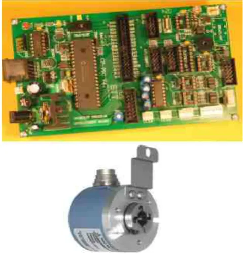
The microcontroller of the speed measurement system determines if $GPRMC string is present and, if so, derives UTC timing from it. As shown on Fig. 2, such UTC times would be 21:50:35 and in 1 sec 21:50:36. Upon deriving each UTC time the microcontroller immediately interrupts the previous speed measurement, sends the result to the output for logging and then with the next command starts the new speed measurement. If GPS is totally unavailable, NMEA messages from the high end geodetic quality GPS receiver would be generated to the timing accuracy reliant on the internal clock of this receiver. Within the logging interval the speed measurement system counts pulses from a speed / distance sensor installed on a wheel as per principles described in [22]. In the experiments described below the sensor represents an industrial encoder WDG 58H of Wachendorff Automation GMBH & Co. The encoder produces 2048 pulses per revolution of the wheel and allows the whole speed measurement system to be accurate in distance measurements as distance calibration is conducted with high degree of accuracy.

The speed measurement system is based on microcontroller PIC18F458 and uses an internal calibration coefficient to convert the number of pulses within 1 sec timing interval, determined by NMEA data, from the speed / distance sensor into speed records. Both the microcontroller board and the industrial encoder used for sensing distance and speed are shown on Figure 3.

Figure 3. Microcontroller board of the speed measurement system and

speed/distance sensor

(6)

synchronization with UTC, the speed records of the test vehicle and all GNSS receivers would fully match in time.

Figure 4. Speed records of the test vehicle

Therefore, the speed measurement system based on microcontroller has a sampling rate of 1 Hz and logs the speed data of the test vehicle with this sampling rate. The GNSS receivers under test have the same sampling rate and therefore are fully synchronized with the test vehicle. This approach addresses the first challenge of synchronizing the speed records between the test vehicle and GNSS receivers under test

The second challenge, which relates to the expected accuracy of the test vehicle, is addressed through separate calibration of distance and time measuring diagrams of the test vehicle, when such diagrams represent the integral parts of the speed measurement system, on a specific test date before and after the test. Also, a thorough UOM analysis was conducted to assess the magnitude of inaccuracies attributed to the test vehicle.

Speed is calculated as distance covered by the test vehicle over a specific time and if both distance and timing diagrams of the test vehicle are properly calibrated, the UOM might be estimated and taken on board when analyzing GNSS speed records.

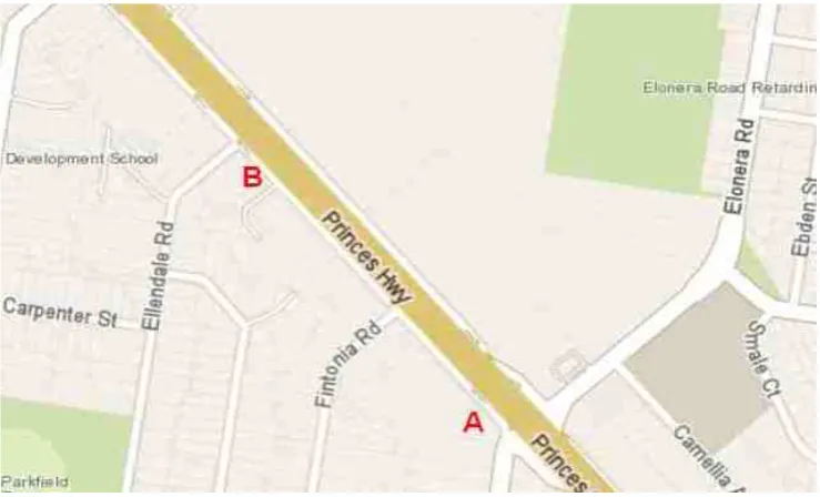
Calibration of the distance measurement diagram is always conducted on a specific test date before and after the test to ensure that the test vehicle stays within the prescribed limits during the test. Distance calibration site represents a straight section of the side road with the surveyed part of 361.3 m shown on Figure 4. This site was surveyed with the Electronic Distance Measurement Unit Leica FlexLine to the accuracy better than 0.002 m. In turn, Leica FlexLine was calibrated with traceability to national distance reference standards. The surveyed section of the road is located in Noble Park area in Melbourne, Australia and is actually going in parallel to Princess Hwy but with almost no traffic as it represents a side road. During distance calibrations the test vehicle is driven from A to B with the speed measurement system working in distance calibration mode.

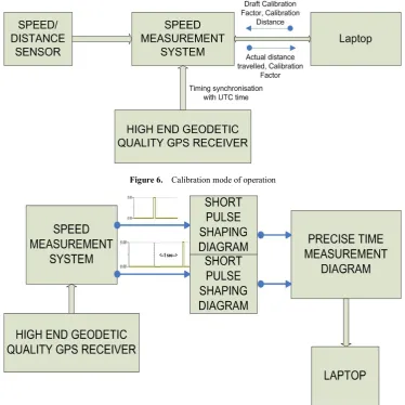
A diagram reflecting the calibration mode for distance measurements is shown on Figure 6.

[image:6.595.120.490.522.746.2]

In distance calibration mode the test vehicle is driven straight from A to B (see Fig. 5) covering a known distance of 361.3 m and the speed measurement system before the drive is loaded with an expected calibration coefficient from the laptop. Laptop in this instance represents also a data logger in this mode of operation and shows the distance measured by the test vehicle rather than speed. If distance measurement conducted by the test vehicle differs by 0.1 m from the actual surveyed distance, a new calibration coefficient is calculated and then loaded with the subsequent drive from A to B again. When a measured distance differs from the surveyed one by less than 0.1 m, distance calibration is complete and the corresponding calibration coefficient loaded on to speed measurement system from the laptop and kept in the microcontroller for the duration of speed tests until the next recalibration.

(7)

[image:7.595.117.492.81.455.2]

Figure 6. Calibration mode of operation

Figure 7. Timing circuit calibration diagram

The UOM of calibration is determined by several prime components and the UOM analysis conducted for calibration uncertainty demonstrated that its value in our experiment equals to 0.2 km/h.

Timing calibration (verification) is conducted with the use of a specific diagram shown on Figure 7. Even in case if 1 sec timestamps are derived from UTC, it is important to ensure that timing inaccuracies are still within the prescribed limits.

Speed measurement system outputs short pulses from the microcontroller, when such pulses constitute the beginning of the new measurement (top output, see Figure 7) and the end of the current measurement (bottom output, see Figure 6). The short pulse corresponding to the beginning of a new speed measurement is generated shortly after every relevant NMEA string of data is produced by the geodetic quality GPS receiver and the microcontroller gets the relevant $GPRMC NMEA string of data. In this instance the microcontroller completes a speed calculation for a previous measurement, puts the speed value to the output

(8)

[image:8.595.121.489.94.291.2]

Figure 8. UFDC-1 in time measurement mode

Timing calibration is achieved here simply via verification that 1 sec timing intervals, dependent on neighboring NMEA data strings are sitting within the prescribed limit to maintain the proper UOM. Usually the measurement time sits within 0.999996 sec and 0.999998 sec as some little time is lost when the microcontroller interrupts the measurement upon the NMEA data string coming, outputs the result of the previous cycle and starts the new cycle of speed measurement. Traceability of UFDC-1 based timing verification diagram to national standards is in turn achieved via checking of its performance with a calibrated pulse generator, for example Agilent 81000, generating pulses on two separate outputs with a known timing shift between them, as shown below.

Figure 9. Traceability check of timing measurement diagram

In this instance a calibrated with traceability to national standards pulse generator verifies that a timing measurement diagram based on UFDC-1 operates within the prescribed limits, i.e. the whole chain of traceability, including for UDFC-1, is maintained

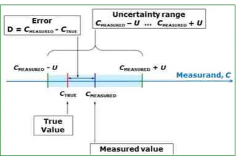
[image:8.595.312.552.322.485.2]

The UOM analysis was conducted for the test vehicle as per methodology described in [24] to determine the UOM in the mode when the vehicle conducts speed tests as shown below.

Figure 10. UOM of the test vehicle

On Figure 10 Cmeasured represents a value of measured speed, Ctrue is a value of the true speed and the uncertainty range is a speed interval where the true values might be with 95% probability and coverage factor 2. In speed mode of operation the test vehicle’s UOM consists of several components with the main ones as follows:

 Calibration uncertainty which is inherited from calibration and equals to 0.2 km/h;

 Number of pulses produced by the speed / distance sensor per one revolution of the wheel and their randomness in regards to 1 sec measurement interval determined by NMEA $GPRMC string;  Changes in tire pressure and its subsequent

circumference when a vehicle is driven at higher speeds due to warm tires;

 Resolution of the speed measurement system;  Variations in timing intervals used as timestamps to

[image:8.595.60.296.503.560.2]

(9)

Based on methodologies described in [24] it was determined that the UOM for the test vehicle in speed measurement mode equals to 0.4 km/h. Both the UOM result as well as producing speed records by the test vehicle in synchronization with speed records generated by GNSS receivers under test allowed to proceed with the actual field speed tests in a variety of environments. Such UOM effectively allowed conducting kinematic testing of GNSS receivers for speed as it is comparable to the performance of GNSS receivers in static mode of operation as shown further in Clause 2.4. Also, quantifying the UOM allowed to further establish the probability of GNSS receivers performing outside of datasheet boundaries in kinematic mode.

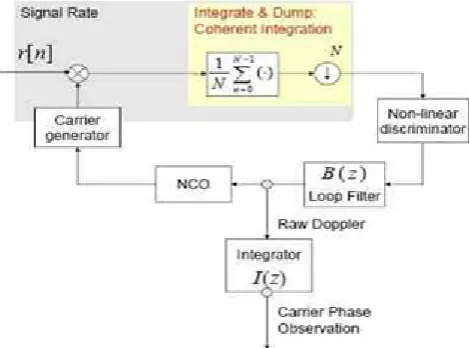
[image:9.595.60.295.329.503.2]

The third challenge in testing GNSS receivers for speed relates to how the receivers determine speed and report it. As discussed above, GNSS receivers primarily use two methods to measure speed: raw Doppler and Carrier Phase. The diagram below represents a general principle of how the receiver determines speed.

Figure 11. Generic speed determination diagram in GNSS receivers

A raw Doppler measurement is a measure of instantaneous velocity, whereas the temporal difference of carrier phase is the measure of mean velocity between observation epochs. Doppler measurements are the direct output of the Phase Lock Loop (PLL) filter and are obtained by processing PLL outputs and therefore parameters such as integration time, loop order and bandwidth strongly impact their quality. However, if the receiver produces internally between 50-100 raw Doppler measurements and only one goes to the output, this specific measurement represents an instant speed at the specific moment. To the contrary, the carrier phase observations are obtained by integrating the raw Doppler measurements. Neither raw Doppler nor carrier phase based measurements represent speed values determined as average within a timing interval of measurement, which is 1 sec determined by NMEA data generation. Moreover, the receivers tested in the below experiment all use raw Doppler method in speed determination and no any test vehicle is capable to produce

50-100 speed records per second in synchronization with UTC as this is not technically feasible. Therefore, it is required to be mindful that speed records of the test vehicle would always represent an average speed value during a measurement interval, say 1 sec, whereas GNSS raw Doppler speed records represent instant speed values at the end of this 1 sec measurement interval. The only method to overcome this challenge is to use only those records for speed assessments where the test vehicle maintains relatively constant speed. Therefore, in this research for the statistical performance calculations of the receivers only those records of the test vehicle were used when neighbouring speed records of the test vehicle generated at 1 sec intervals differ in speed values by no more than the UOM of the test vehicle. This effectively means that records when the test vehicle accelerates or slows down by more than 0.4 km/h within 1 sec are filtered out and only smooth driving related records are used for further assessments.

2.4. Static Speed Tests

Before commencing kinematic tests, the receivers were tested for their static performance to ensure their speed errors are known in ideal conditions, i.e. in open sky environments when the receivers were stationary, and in almost ideal conditions when the receivers were stationary but located in different locations, for example, when the test vehicle was staying on traffic lights or emergency lanes off the roads.

The following GNSS receivers were tested during the static and further kinematic tests:

 High end GPS only receiver (Receiver 1);

 High end GNSS receiver with GPS and GLONASS enabled (Receiver 2);

 Medium range GPS only receiver (Receiver 3);  Low grade GPS only receiver (Receiver 4).

Note 1. In further discussion GNSS receivers would mean not only the devices showing GNSS data on their displays but also the devices capable of logging the data either on SD-cards or via any output ports. Such devices are widely available to general public and researchers.

(10)

rather than benefit and DGPS would disadvantage the other receivers under test. Considering that in practice the majority of consumer grade receivers do not use DGPS, it is unfair to test different receivers in different modes of operation. The Receiver 2 is similar to the Receiver 1 but is capable to use L1 frequency only. Both Receivers 1 and 2 had very complex software manuals providing a capability for the user to use several hundred commands to configure the Receivers via changes in GNSS settings. Hence, the Receivers 1 and 2 were configured to use the raw Doppler method to compute speed records and output NMEA data with speed values via RS232 ports every second with the resolution of several digits after the decimal point. Also, both Receivers 1 and 2 had external GNSS antennas mounted on the roof of the test vehicle and were configured with 15 degrees masking angle. The manufacturer’s datasheets for these receivers claimed that they can measure speed with the accuracy of 0.11 km/h Root-Mean-Square (RMS).

The Receiver 3 was a GPS logger recording speed every 10 milliseconds on its own SD card with a number of digits after the decimal point and with an internal GPS antenna. This Receiver belongs to medium range because it does not allow the user to change any GPS settings to configure the Receiver in a way the user wants. Therefore, all GNSS settings were hardcoded to the Receiver by the manufacturer. Also, the Receiver 3 does not have a capability to output NMEA data and therefore there was no option to understand the number of parameters, such as the specific satellites used by this receiver for conducting each speed measurement, HDOP values and signal to noise ratio (SNR) for these satellites. At the same time the receiver is capable to work with IPhone via Bluetooth where a performance test application might be used on smart phone to work with the data. Also, the receiver is flexible in the use of either the internal or external GPS antenna and it uses a 20 Hz GPS engine. The Receiver 3 was located on the dashboard of the test vehicle as allowed by the manufacturer and the mask angle for this receiver was hardcoded by the manufacturer to 7 degrees. The manufacturer’s datasheets for this receiver claimed that the Receiver can measure speed with the accuracy of 0.1 km/h without specifying the environmental GPS related conditions when such accuracy can be achieved. The cost of this Receiver was approximately $500.

The Receiver 4 represented a low grade GPS receiver because of multiple factors, such us: no ability to change configuration settings by the user, no ability to use an external GPS antenna and very limited logging capability in terms of GPS parameters. This GPS receiver’s cost was $70 and it logged GPS speed every second with integer speed values on its own SD card using CSV file rather than NMEA. Therefore, for this receiver it was also not possible to derive which specific satellites were used at any specific times for navigation and speed measurements, their SNR and many other parameters available through NMEA data. However, with each speed record the receiver outputted a number of parameters, such as UTC, number of satellites used, HDOP and some others. It also had an internal antenna and therefore

the Receiver 4 was mounted on the dashboard of the test vehicle. For this receiver the manufacturer did not specify the speed accuracy parameter. It is required to note that for GPS Receivers 3 and 4 the datasheets allow the installation of Receivers on the dashboard and hence the manufacturers of the Receivers shall guarantee the performance of their products in such instances as per datasheet parameters.

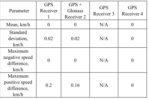
The receivers during the static tests were stationary. At the same time they reported minor variations in speed and their speed difference parameters are shown in the below tables

Table 1. Speed errors in static conditions and ideal open sky

environments

Parameter Receiver GPS 1

GPS + Glonass Receiver 2

GPS

Receiver 3 Receiver 4 GPS Mean, km/h 0 0 N/A 0

Standard deviation,

km/h 0.02 0.02 N/A 0 Maximum

negative speed difference,

km/h

0 0 N/A 0

Maximum positive speed

difference, km/h

0.2 0.16 N/A 0

Note. GPS Receiver 3 did not produce static speed records because of the internal accelerometer preventing the receiver to produce stationary speed records. GPS Receiver 4 produced very good static results simply because the Receiver does not generate speed records with decimal points and effectively all values were rounded to zero.

Table 2. Speed errors in static conditions and non-ideal GNSS

environments

GPS + Glonass Receiver 2

GPS

Receiver 3 Receiver 4 GPS

Mean, km/h 0 0 N/A 0 Standard

deviation,

km/h 0.04 0.04 N/A 0 Maximum

km/h

-0.3 -0.4 N/A 0

difference, km/h

0 0 N/A 0

Note. Almost ideal conditions mean generally open sky environments but some obscurations are still possible providing no less than 4 satellites visibility.

[image:10.595.313.553.229.390.2] [image:10.595.313.551.460.619.2]

(11)

respectively. The number of outliers sitting beyond the boundaries prescribed in the datasheets was 113 for the Receiver 1 and 66 for the Receiver 2.

Results from speed tests conducted in static conditions and the UOM of the test vehicle allowed to further progress with kinematic tests.

2.5. Kinematic Speed Tests

The test to determine speed accuracy parameters and outliers generated in kinematic mode was conducted in February 2015 on a specific route consisted of freeways with a number of overpasses, suburban areas and countryside roads where tree canopies covered some sections of the roads alongside with open sky sections. The test vehicle was driven from Melbourne to Echuca and covered slightly less than 250 km.

To eliminate any potential causes of systemic errors which might be experienced by all receivers on the day the following measures were put in place:

a/ space weather advisories were analyzed to confirm that within the test time there were no events which could potentially impact the performance of the receivers under test;

b/ GPS Notice Advisory to NAVSTAR Users (NANU) Reports and GLONASS advisories were analyzed to confirm that the integrity of the GPS and GLONASS constellations was maintained for the duration of the test;

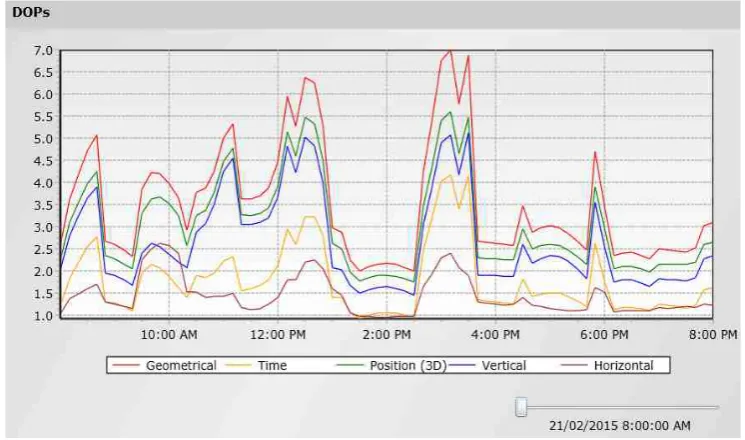
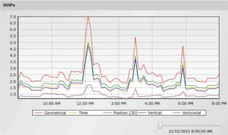
[image:11.595.121.490.286.500.2]

c/ with help of GNSS planning software an analysis was conducted to confirm the satellites availability in Victoria and Dilution of Precision (DOP) parameters for the duration of the test and eliminate possible systemic problems. The below plots indicate the results:

Figure 12. GPS and GLONASS satellites availability in test area during the test

[image:11.595.118.491.521.741.2]

(12)

[image:12.595.120.488.79.297.2]

Figure 14. GPS and GLONASS DOP predicted availability during the test

It is visible from the above plots that for GPS only receivers the number of predicted satellites varies from five to eight and for GPS +GLONASS receivers from nine to 15 in open sky ideal conditions. Also, predicted HDOP for GPS only receivers is no more than 2.5 and for GPS+GLONASS receivers is no more than 1.75 in open sky ideal conditions. All the above demonstrates that systemic causes of errors related to GNSS availability in the area are eliminated.

The test vehicle represented a vehicle Mazda 3 hatchback with the speed measurement system calibrated before the test as per methodologies described in 2.3. For the entire test the speed measurement system of the test vehicle was operational. After the test the speed measurement system was checked for the correctness of distance and time measurements.

3. Results

3.1. Statistical Performance

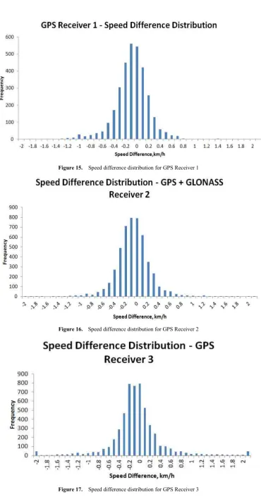
Figures 15-18 demonstrate speed difference distributions for the Receivers 1, 2, 3 and 4 respectively, i.e. the number of speed records of the GNSS Receivers corresponding to the specific speed errors, when such errors were measured as differences between the calibrated test vehicle speed records and the relevant speed records of GNSS Receivers. Such distributions were put in place taking into account smooth

[image:12.595.313.553.494.656.2]

driving records of the test vehicle only as discussed in Clause 2.3, i.e. only those records of the test vehicle when the speed difference between neighboring 1 sec records is less than the UOM of the test vehicle. Also, speed outliers generated around overpasses were eliminated from the assessment as they are separately analyzed in the next Clause 3.2. Finally, speed records when the test vehicle was stationary were also eliminated from the assessment as they may change the statistical performance dramatically due to differences in static measurements caused by rounding in the GPS Receiver 4. Statistical analysis for speed differences is provided in Table 3.

Table 3. Statistical performance in kinematic conditions

GPS + GLONASS

Receiver 2

GPS Receiver

3

GPS Receiver

4 Mean, km/h -0.1 -0.1 -0.1 0.4

Standard deviation,

km/h 0.3 0.3 0.7 0.5 Maximum

km/h

-3.5 -2.8 -11.3 -3.1

difference, km/h

(13)

Figure 15. Speed difference distribution for GPS Receiver 1

[image:13.595.122.493.52.768.2]

[image:13.595.121.498.85.281.2]

(14)

3.2. Speed Outliers

Table 4 below demonstrates the magnitude and the number of speed outliers generated by the Receivers 1-4 under test for the entire test drive only around overpasses with some locations of their generation shown on the relevant Figures below.

[image:14.595.312.550.81.213.2] [image:14.595.62.292.81.230.2]

Note. An outlier is a measurement that is distant from other measurements. As GNSS receivers are generally very precise in speed measurements, any GNSS speed measurement with an error of several kilometers per hour is considered to be an outlier.

Table 4. Average GNSS speed spikes for overpasses and the number of

spikes during the test

Receiver GPS 1

GPS + GLONASS

Receiver 2

GPS Receiver

3

GPS Receiver

4 Average speed

difference between the test

vehicle and the receiver under

test, km/h

5.35 4.74 10.7 10.5

Number of

outliers 7 10 30 23

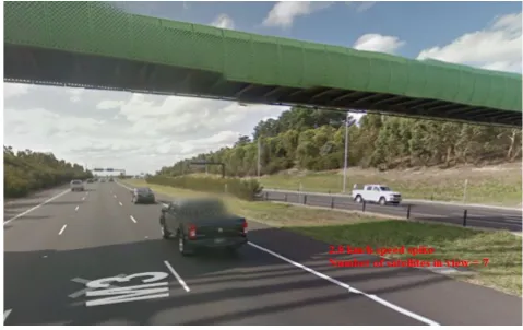
Figure 19. Example of the environment where an outlier was generated

by the GPS Receiver 1

[image:14.595.311.551.248.399.2]

[image:14.595.58.297.430.699.2] [image:14.595.313.552.434.590.2]

(15)

In addition to the outliers generated around overpasses, the GPS Receiver 3 only generated 122 outliers in the countryside on road sections with tree foliage environments. The average magnitude of such outliers was equal to 3.8 km/h. Trees can potentially be a significant source of GNSS signal loss, and there are a number of parameters involved, such as: the specific type of tree, whether it is wet or dry, and in the case of deciduous trees, whether the leaves are present or not. It was expected that even isolated trees might represent a problem for GNSS signals; however, a dense group of trees or trees staying all along a particular section of the road might represent a major problem. The expectation was based on the fact that the attenuation of signals in general depends on the distance the signal must penetrate through the forest or leaves, and the attenuation increases with frequency. The attenuation generally is of the order of 0.05 dB/m at 200 MHz, 0.1 dB/m at 500 MHz, 0.2 dB/m at 1 GHz, 0.3 dB/m at 2 GHz and 0.4 dB/m at 3 GHz. As GNSS L1 frequency equals to 1575.42 MHz, the GNSS signal sits in the middle of Ultra High Frequency (UHF) range and therefore is vulnerable to propagation along tree lined roads. It is important to highlight; however, that the behavior in outliers generation in their large numbers was not observed for high end Receivers 1 and 2 and low range Receiver 4. This highlights the fact that it is very important to test GNSS receivers in a number of real world environments to reveal their true behavior.

3.3. Reliance on Speed Records based on HDOP only

[image:15.595.312.553.183.302.2]

The equation (5) mentioned in 2.2 may create an impression that it might be possible to filter unreliable GNSS speed records based on HDOP and use HDOP as a potential quality indicator for speed records. This approach generally works for GNSS position records with no multipath where positional measurements are rated based on HDOP in a way as follows [25]:

Table 5. Positional accuracy depending on HDOP

HDOP Rating Description

<1 Ideal The highest possible confidence level 1-2 Excellent Positional measurements are _{considered accurate enough}

2-5 Good Positional measurements could be used to make reliable in-route navigation suggestions

5-10 Moderate Positional measurements could be used for calculations but the fix quality could still be improved 10-20 Fair Positional measurements should be _discarded

>20 Poor Measurements are very inaccurate

The task of further investigation was to consider if it is possible to put a similar table for GNSS speed records considering their dependency on HDOP as per the equation (5). In other words, the goal in here is to determine, if any, a certain HDOP threshold when it might be possible to

confirm that speed records are potentially unreliable. Each speed outlier produced by geodetic quality Receivers 1 and 2 was analyzed to get an indication if the number of satellites or HDOP parameters might be helpful to indicate a problem. Tables 6 and 7 below represent each individual outlier with GPS parameters derived from NMEA data.

Table 6. GPS parameters for speed outliers produced by the GPS

Receiver 1

HDOP Number of Satellites Speed Difference, km/h

9.3 4 -6.02

26.3 4 7.60

4.8 4 6.14

7.4 4 4.38

2.1 6 5.41

2.2 6 2.57

1.6 7 5.33

Table 7. GPS parameters for speed outliers produced by the GPS

Receiver 2

HDOP Number of Satellites Speed Difference, km/h

1.6 7 -2.74

1.1 11 2.75

0.9 12 2.51

7.2 6 3.85

9.2 6 5.87

1.2 8 -2.92

1.2 11 9.6

1.1 12 6.07

It is seen from the above tables that speed records with high values of HDOP might be used to potentially indicate a problem in speed accuracy. However, for some records the low HDOP values are not indicating an issue in speed measurements, whereas the speed spikes are present. Considering that the equation (5) is always correct, this effectively means that due to multipath around overpasses the receivers output HDOP incorrectly, i.e. the calculated and outputted HDOP values are affected by multipath. Therefore, from the integrity point of view it is much safer to exclude such speed records around overpasses from the assessment rather than rely on them even in case if HDOP values do not indicate a problem. The same results were observed for the GPS receiver 4. GPS receiver 3 does not have any DOP parameter logged with speed records and therefore it was not possible to assess each spike and understand why it was produced. However, looking at number of satellites for each speed spike it was again not possible to conclude that the receiver experienced problems at specific epochs when spikes happened.

[image:15.595.312.553.332.466.2] [image:15.595.58.298.544.695.2]

(16)

[image:16.595.58.299.319.467.2]

At the same time, considering the equation (5), it is still possible to use HDOP as a statistical indicator of reliability of speed records. To demonstrate this possibility a different test was conducted with the Receivers 1 and 4 only with a focus on countryside roads where tree foliage environments were more present. As a result of trees reducing GNSS signals, such test provided much worse GNSS visibility in comparison to the previous test and therefore HDOP would definitely vary within a broader range due to a variety of GNSS environments. For the test day an assessment of GNSS environment using space weather, NANU reports and GNSS plotting was conducted in a manner described in clause 3.4 with no GNSS issues identified. Subsequently, examination of the data was conducted with filtering of speed records for different HDOP intervals and deriving statistical speed errors depending on HDOP values. Findings obtained from the test are as follows:

Table 8. Standard deviation of the speed error for the GPS Receiver 1 as

a function of HDOP

HDOP range value Standard Deviation of Speed Error, km/h All range of HDOP 0.92

HDOP<=1 0.24

1.1 - 2 0.39

2.1 – 3 0.82

3.1 – 4 1.01

4.1 – 5 1.32

5.1 – 6 1.12

6.1 – 7 1.51

HDOP>7 4.27

Table 9. Standard deviation of the speed error for the GPS Receiver 4 as

a function of HDOP

HDOP range value Standard Deviation of Speed Error, km/h

HDOP<=1 0.7

1.1 - 2 1.6

2.1 – 3 6.4

HDOP>3 4.4

There is a clear statistical dependency of the speed error of GPS Receivers 1 and 4 on HDOP. Considering the datasheet for the Receiver 1 and the UOM of the test vehicle, only speed records with HDOP up to 2 might be considered as reliable for the geodetic quality GPS Receiver 1. For the GPS Receiver 4 the situation with the HDOP threshold is even worse compared to the Receiver 1 and only records with HDOP <=1 might be statistically considered as reliable. With HDOP higher than one a speed error of this receiver sharply increases and the actual speed errors, going up to two standard deviations for the majority of records, would be sitting outside of plus/minus 3 km/h range. Such errors are not what the consumers expect to see from GPS receivers, although everything depends on the application. Also, the results shown in Tables 8 and 9 indicate that for speed

records it is not possible to put a table similar to Table 5 where reliance on records might be guaranteed based on HDOP.

4. Discussion

4.1. Statistical Performance

It is evident that despite the fact that all receivers use an embedded generic raw Doppler based algorithms to determine speed, their statistical performance demonstrates significant differences between the receivers. Considering the values of standard deviations of speed errors produced by different receivers as shown in Table 3 and relevant speed error distributions, it is possible to say that for geodetic quality receivers the reported speeds for the vast majority of records sits within 0.6 km/h from the true speed, whereas for mid range Receiver 3 and low grade Receiver 4 such reported speed records are within 1.4 km/h and 1 km/h respectively, i.e. within two standard deviations of the speed error

Remembering that the UOM of the test vehicle for speed measurements equals to 0.4 km/h and that in stationary mode geodetic quality Receivers 1 and 2 demonstrated their performance within ±0.1 km/h as per their datasheets, it is very likely that the statistical performance of such receivers is compliant to the datasheets in regards to speed accuracy. This is because in the worst situation the combined UOM of the test vehicle and the static speed noise might be up to 0.5 km/h, which differs from ±0.6 km/h speed range by only 0.1 km/h.

Unlike the Receivers 1 and 2, the Receiver 3 is non-complaint to its datasheet speed accuracy parameter simply because the Receiver’s speed values sit in the interval of ±1.4 km/h from the true speed. Considering the UOM of the test vehicle, the Receiver 3 still expressed the behavior when ±1 km/h speed variations in its reporting are attributed to the Receiver rather than the test vehicle

4.2. Difference in Generation of Outliers

(17)

and Horizontal Dilution of Precision (HDOP) in the relevant speed records.

The use of GLONASS in the Receiver 2 did not significantly improve the performance in terms of both speed accuracy and the number of outliers but obviously increased the number of valid speed records in general. The average speed error for such outliers was 4.7 km/h for the GPS+GLONASS Receiver 2 compared to 5.3 km/h for GPS only Receiver A. This improvement is very marginal. It is required to highlight that the number of outliers, i.e. seven and 10 outliers produced by geodetic quality Receivers 1 and 2 within the entire run, is still high in their magnitude (see Table 4) because the average speed errors of 5.35 km/h and 4.74 km/h are not what the consumer would generally expect from such type of receivers.

For medium range and low grade Receivers 3 and 4 the situation with speed accuracy around overpasses is much worse as these Receivers have average speed errors for their outliers equal to 10.7 km/h and 10.5 km/h (see Table 4) and the number of outliers is relatively high. The above results highlight that the use of speed records, when they are produced around overpasses or even narrow bridges for pedestrian crossing (see Fig. 21) might not be justified. The fact that the Receiver 3 produced also 122 outliers in the countryside measuring speed on sections with tree canopies with an average error of 3.8 km/h highlights that some GPS receivers may not be even metrologically trusted in such environments.

4.3. Integrity of GNSS Speed Records based on HDOP

Tables 6 and 7 prove that it is not possible to rely on HDOP values when analyzing each individual speed records for its integrity. HDOP values in the areas where multipath is present and specifically around overpasses might be misleading. This is because the reflected GNSS signal from one or two specific satellites makes HDOP value looking good, whereas the real value of HDOP simply cannot be calculated by the receiver correctly. Tables 8 and 9 indicate that it is challenging to derive specific generic HDOP thresholds and classify GNSS speed records for their integrity based on such thresholds. Every type of GNSS receiver with its settings might have its own HDOP thresholds corresponding to integrity intervals in GNSS speed measurements.

5. Conclusions

Testing of GNSS receivers for speed represents a number of challenges. The first challenge relates to high accuracy in speed measurements claimed by the manufacturers of GNSS chipsets and receivers in the relevant datasheets. The second challenge is linked to the necessity of timing synchronization between the test vehicle speed records and speed records generated by GNSS receivers. The third challenge relates to the algorithm how the receivers determine and output speed,

when speed records might be generated with high frequencies and speed values effectively represent immediate speeds rather than speed calculated over time. In this paper a design of the test vehicle is proposed when an electronic system of this vehicle is capable to test GNSS receivers for speed. The proposed electronic speed measurement system addresses all challenges of testing GNSS receivers and provides a combined UOM of the test vehicle equal to 0.4 km/h. Subsequent speed tests of GNSS receivers validated that their speed errors might be relatively high around such structures as overpasses where multipath might disturb the correctness of speed measurements or in tree foliage environments where GNSS signals degrade. In this specific research while high end geodetic GPS and GNSS specific receivers performed generally better in multipath related environments than medium range and low grade receivers, they still occasionally experienced speed spikes of up to several km per hour, including in instances when they are configured with relatively high elevation mask filtering. Medium range and low grade GPS receivers generated relatively substantial number of measurement outliers around overpasses with up to 10 km/h reported errors in speed measurements. In addition, the medium range receiver generated relatively high numbers of outliers in the areas where tree canopies surround some sections of the road. This conclusion, however, should not be generalized and conducting an independent speed testing of each type of receiver to reveal its true performance in the real world environments is encouraged. Also, specific GNSS conditions, i.e. presence of overpasses, trees and other structures should be analysed when looking at a specific GNSS speed record to determine the level of its integrity.

Secondly, after adding GLONASS to a GPS-only solution, an improvement was obviously seen in GNSS availability and increased number of valid speed records thanks to additional GLONASS satellites used to compute speed records. However, the benefit of enabling additional GNSS constellations and specifically GLONASS to complement GPS in speed measurements in terms of improving GNSS speed errors is very marginal. This is concluded from the ratio of the relative number of outliers to all valid speed records when such ratio improved from 0.09% to 0.08% and the average speed error of such outliers decreased from 5.3 km/h to 4.7 km/h.

(18)

REFERENCES

[1] R. Wainright. Farther and son stick to guns to prove radar wrong, The Sydney Morning Herald, Online available from <http://smh.com.au>, 12 March 2007.

[2] N. Truebridge. GPS speeds accurate, Online available from <http://www.stuff.co.nz>, 12 December 2014.

[3] D. Huang. Evidential Problems with GPS Accuracy: device Testing, A Thesis submitted to the Graduate Faculty of Design and Creative Technologies in partial fulfillment of the requirements for the Degree of Master of Forensic Information Technology, School of Computer and Mathematical Sciences, Auckland, New Zealand, 2013. [4] T. Chalko. Estimating accuracy of GPS Doppler speed

measurement using Speed Dilution of Precision (SDOP) parameter, Online available from<http://www.nujournal.net/ SDOP.pdf>.

[5] K. Taylor, M. Schrock, J. Bloomfield et al. Dynamic testing of GPS receivers, The Society for Engineering in Agricultural, Food and Biological Systems, an ASAE Meeting Presentation, Paper Number 03-1013, 2004.

[6] T. Witte, A. Wilson. Accuracy of non-differential GPS for the determination of speed over ground, Journal of Biomechanics, Vol.37, pp. 1891-1898, 2004.

[7] G. Ogle, R. Guensler, W. Bachman et al. Accuracy of Global Positioning System for determining driver performance parameters, Transportation Research Record 1818, Paper No02-1063, 2002.

[8] K. Al-Gaadi. Testing the accuracy of autonomous GPS in ground speed measurements, Journal of Applied Sciences, Vol.5, pp. 1518-1522, 2005.

[9] A. Chowdhury, T. Chakravarty, P. Balamuralidhar. Estimating true speed of moving vehicle using smartphone based GPS measurement, Conference Proceedings – IEEE International Conference on Systems, Man and Cybernetics, article. No 6974444, pp. 3348 – 3353, 2014.

[10]W. Ding, J. Wang. Precise velocity estimation with a standalone GPS receiver, Journal of Navigation, Vol.64, pp.311-325, 2014.

[11]Y. Bai, Q. Sun, L. Du, M. Bai. Two laboratory methods for the calibration of GPS speed meters, Measurement Science and Technology, Vol.26, 2015.

[12]A. Dyukov. GNSS based vehicle speed determination, Australian ITS Summit Proceedings – ITS Australia, presentation S14, Online available from<http://www.itsaustr

alia.com.au>, 2013.

[13]D. Sathyamorthy, S. Shafii, Z.M. Amin, A. Jusoh, S.Z. Ali. Evaluation of the accuracy of global positioning system (GPS) speed measurement via GPS simulation, Defense S and T Technical Bulletin, 8(2), pp.121-128, 2015.

[14]Correvit SFII Sensors Non-Contact Optical Sensors, CSF2A_000-812e-02.15, 2015.

[15]M. Keskin, Y. Sekerli, S. Kahraman. Performance of two low cost GNSS receivers for ground speed measurements under varying speed conditions, Vth International Scientific Symposium for PhD Students and Students of Agricultural Colleges, Poland, 18-20 September 2014.

[16]MAX-6 Ublox 6 GPS Modules, Datasheet.

[17]SIRFStarIV GSD4E, High-sensitivity GPS location processor with built-in CPU and SiRFaware Technology, Product Overview.

[18]A. Durant, M. Hill. Technical assessment of the DL2S GPS data quality including comparative data from VBOX3 (with optional DGPS) and an optical speed sensor, race Technology Ltd, May 2005.

[19]M. Bahrami. GNSS Doppler positioning (an overview), University College London, Geomatics Lab, a Paper prepared for GNSS SIG Technical Reading Group, 12 p.

[20]J. Zhang. Precise velocity and acceleration determination using a standalone GPS receiver in real time, RMIT University, School of Mathematical and Geospatial Sciences, 2007.

[21]Global Positioning System Standard Positioning Service Performance Standard, 4th_{Edition, 160 p., 2008.}

[22]R. Vishanathan. Evaluation of ground speed sensing devices under varying ground surface conditions, Submitted to the Faculty of Graduate College of the Oklahoma State University in the partial fulfillment of the requirements for the Degree of Master of Science, July 2005.

[23]Universal frequency to digital converter (UFDC-1), Specification and Application Note, International Frequency Sensor Association (IFSA).

[24]Measurement uncertainty estimation, a three day short course for laboratory and testing staff based on ISO Guide to the Expression of Uncertainty in Measurements, Course No008, Metrology Training International Pty Ltd.