Optimization of Process Planning and Scheduling using ACO and PSO Algorithms

(1)

International Journal of Emerging Technology and Advanced Engineering

Website: www.ijetae.com (ISSN 2250-2459, Volume 2, Issue 10, October 2012)

343

Optimization of Process Planning and Scheduling using ACO

and PSO Algorithms

P. S. Srinivas

1

, V. Ramachandra Raju

2

, C.S.P Rao

3

1_{Asso. Prof., V.R. Siddhartha Engg. College, Vijayawada}

2_{Professor, JNTUCE - Vjayanagaram}

3_{Professor, Department of Mechanical Engg., NIT, Warangal}

Abstract - The decision of selecting a process plan in a manufacturing system is crucial and the generated process plan need not be the best possible sequence in a changing production environment. As the complexity of the product increases, the number of feasible sequences increases exponentially and there is a need to choose the best among them. The process planning is modeled as a combinatorial optimization problem with constraints, and an Ant colony optimization (ACO) approach has been used to achieve the global lowest machining cost. Scheduling is concerned with allocating limited resources to tasks to optimize some performance criterion, such as completion time or production cost. Scheduling of a job shop is very important in both fields of production management and combinatorial optimization. However, it is quite difficult to achieve an optimal solution to this problem with traditional optimization approaches owing to the high computational complexity. A large number of approaches to the modeling and solution of these scheduling problems have been reported with varying degrees of success. Exact solution methods are unfeasible for most problem instances and heuristic approaches must therefore be employed to find good solutions with reasonable search time. Particle Swarm Optimization (PSO) methodology is adopted for solving a job shop problem with an objective of minimizing the makespan. In this paper the integration of Process Planning and Scheduling is attempted to get the lower minimum manufacturing cost and minimum makespan for the products.

Keywords - Process Planning, Ant Colony Optimization, Precedence Relationship matrix, Job Shop Scheduling, Particle Swarm Optimization, Makespan.

I. INTRODUCTION

One of the most important steps in converting the raw material to the finished product economically and competitively is process planning. Process Planning activities include selection of machining processes, selection of machine tools, operation sequence, selection of cutting tools, determination of the cutting conditions, determination of setup requirements, selection of jigs and fixtures, calculation of process times, Tool path planning & NC program generation, generation of process route sheets.

The routing becomes a major input to the manufacturing resource planning.

The generation of various feasible plans and to find the best among them constitutes an NP-complete combinatorial problem. Hence an efficient heuristic search is required to solve such problem. We applied the ant colony algorithm to solve the problem of generating optimal process plan for some parts. The approach models process planning considering the machine, tool, and tool approach directions for each operation. Precedence relationships are the constraints for the solution space. The optimal process plan is found based on the minimum total cost criteria.

Scheduling is the allocation of resources to accomplish the processes identified by the process planner. The Optimum utilization of the available resources is a challenging task here. The Job Shop Scheduling is considered to be NP hard problem and one of the hardest combinatorial problems to solve and it is quite difficult to achieve an optimal solution to this problem with traditional optimization approaches owing to the high computational complexity.

II. NEED FOR INTEGRATION OF PROCESS PLANNING AND

SCHEDULING

Often process planning and scheduling have conflicting objectives. Process Planning emphasizes the technological requirements of a task, while Scheduling involves the timing aspects of it (Manish, 2003). The information generated by the process planning activities is used as the inputs of scheduling. Therefore, the process planning becomes an unavoidable constraint for scheduling. In this paper the process planning and scheduling are integrated to achieve the optimum cost and the minimum makespan.

III. LITERATURE

(2)

International Journal of Emerging Technology and Advanced Engineering

344

They communicate between each other using chemical substances, the pheromones. This indirect communication allows the entire colony to perform complex tasks, such as establishing the shortest route paths from their nests to feeding sources. In (Dorigo et al. 1996) an optimization algorithm was proposed that tries to mimic the foraging behavior of real ants, i.e. the behavior of wandering in the search for food. This algorithm has already been successfully used to solve the TSP (Gambardella and Dorigo 1996), and other NP hard optimization problems (Silva et al. 2002).

Shen W wt al (2006) describes the complexity of manufacturing process-planning and scheduling problems, and reviews the research literature in manufacturing process planning, manufacturing scheduling, and the integration of process planning and scheduling, particularly focusing on agent-based approaches in these areas.

Krishna A.G and Mallikarjuna Rao, 2006 presents an application of a newly developed meta-heuristic called the ant colony algorithm as a global search technique for the quick identification of the optimal operations sequence by considering various feasibility constrains. A couple of case studies are taken from the literature to comparing the results obtained by the proposed method.

Jain P.K and V.K Gupta use ant colony optimization technique to solve the operation sequencing problem. Their approach analyses the precedence relationships among features to generate a precedence relationship matrix (PRM). The operation-sequencing problem in process planning is considered to produce a part with the objective of minimizing the sum of machine, setup and tool change costs.

Li et al 2002 proposed a hybrid genetic algorithm (GA) and simulated annealing (SA) approach to consider concurrently the processes of selecting machining resources, determining set-up plans and sequencing operations for a prismatic part in an optimization procedure.

Tiwari M.K et al used GA to obtain a set of process plans for a given variety of parts and production volume with the objective of minimizing the total processing time, setup time and material handling time constrained by not overloading the machines.

Kennedy J, Eberhart R C [3] are the first persons introducing this particle swarm optimization. It is an evolutionary computation technique mimicking the behavior of flying birds and their means of information exchange. It combines local search (by self experience) and global search (by neighboring experience), possessing high search efficiency.

Chandrasekaran. S et al [2] dealt the problem of scheduling in flow shops with the objective of minimizing makespan, total flow time and completion time variation. Rahimi [4] considered a bi-criteria permutation flow shop scheduling problem, where weighted mean completion time and weighted mean tardiness are to be minimized simultaneously. Since a flow shop scheduling problem has been proved to be NP-hard in strong sense, an effective multi-objective particle swarm (MOPS), exploiting a new concept of the Ideal Point and a new approach to specify the superior particle‘s position vector in the swarm, is designed and used for finding locally Pareto-optimal frontier of the problem.

Zhixiong Liu [7] proposed the particle representation based on operation-particle position sequence. In the particle representation, the mapping between the particle and the scheduling solution is established through connecting the operation sequence of all the jobs with the particle position sequence. The particle representation can ensure that the scheduling solutions decoded are feasible and can follow the particle swarm optimization algorithm model. Weijun Xia and Zhiming Wu proposed a hybrid optimization approach for multi objective flexible job shop scheduling problems, where they can integrate particle swarm with simulated annealing for solving job shop problems. By reasonably hybridizing these two methodologies, they develop an easily implemented hybrid approach for the multi-objective flexible job-shop scheduling problem (FJSP).

Sha and Cheng [5] proposed a hybrid particle swarm optimization (PSO) for the job shop problem. Since the solution space of the JSP is discrete, we modified the particle position representation, particle movement, and particle velocity to better suit PSO for the JSP.

In this paper, we propose an approximate method to resolve a multi product batch flow shop schedule.

This paper is divided in to two sections. The first section describes the ant colony algorithm (AC) and the method to generate a population of the optimal sequences. The second section deals with the scheduling to get the minimum makespan for the job shop scheduling problem and these two are integrated.

IV. ACOIMPLEMENTATION

(3)

International Journal of Emerging Technology and Advanced Engineering

345

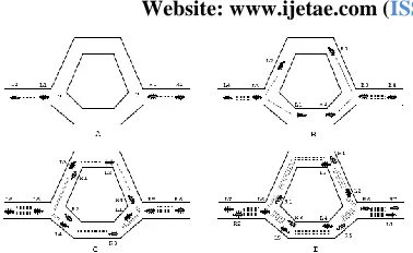
Figure 4.1: How real ants find a shortest path. A) Ants arrive at a decision point. B) Some ants choose the upper path and some the lower path. The choice is random. C) Since ants move at approximately constant speed, the ants which choose the lower, shorter, path reach the opposite decision point faster than those which choose the upper, longer, path. D) Pheromone accumulates at a higher rate on the shorter path. The number of dashed lines is approximately proportional to the amount of pheromone deposited by ants.

In the Ant Colony Optimization (ACO) metaheuristic a colony of artificial ants, cooperates in finding good solutions to difficult discrete optimization problems. Cooperation is a key design component of ACO algorithms and good solutions are an emergent property of the ant's cooperative interaction. The technique involves observing the part feature details form available drawings, and operations required for each feature, and also precedence relations among operations. Generate 'A' number of artificial ants, where 'A' is assumed to be equal to the number of operations 'n'. Set initial value of pheromone (

Q







--- (1)

Where, Q is a pheromone deposition constant. In the present study, a value of '10' was taken from literature. FFk

is the value of the objective function for the sequence under consideration (i.e. sequence generated by kth ant). Reduce pheromone on the edges of incomplete sequences to weaken it chances for selection in the next iteration. The following expression is used to reduce the pheromone on the edges of an incomplete sequence.

ij





also avoids unlimited accumulation of the pheromone trails on the edges and thus allows the algorithm to forget previously done bad choices. Researches in the past have used a range of values for



varying from '0' to '0.5', but in our algorithm a value of 0.1 for



has taken. After each iteration the pheromone updation and evaporation takes place after certain number of iterations or position values of each operations are not improving then pick the highest pheromone position for each operation according to precedence constraints, this is the best sequence.

A. Precedence relationship between operations

The Precedence Relationships (PR‘s) between operations come from geometrical and technological consideration to produce every feature with the best possible accuracy. Some constraints are:

 Fixture Requirement: Precedence relationship between two features exists when machining one feature first may cause another to be unfixturable.

 Datum Requirement: When two features have a dimensional or geometrical tolerance relationship, the feature containing the datum should be machined first.

 Good Manufacturing Practice: Good manufacturing practice or rules-of-thumb may also result in precedence relationships between features.

[image:3.612.75.264.121.237.2]

(4)

International Journal of Emerging Technology and Advanced Engineering

346

B. Criteria for optimizing the optimizing the precedence

sequence

The precedence sequence optimization is based on the weighted cost, which consists of

Machine cost,





n i i

MCI

MC

1 --- (3)

Where n is the total number of Operations and

MCI

_i is the machine cost index for using machine-i.

Tool cost,



  n i i TCI TC 1 ---(4)

Where

TCI

_i is the tool cost index for using tool i

Machine Change Cost (MCC): a machine change is needed when two adjacent operations are performed on different machines,



  









1 1 1

))

(

1 (

*

n i i i

M

MCCI

MCC

-- (5)

Where MCCI is the machine change cost index, and Mi

is the machine ID used for operation i.

Where



1 0

1

)

(









M

_i_₁

Setup change cost (SCC): A setup change is needed when two adjacent Operations performed on the same machine have different TADs.



          1 1 1

1 ))* ( ))

( 1 (( * n i i i i

i M TAD TAD

M SCCI

SCC

- (7)

Where SCCI is the setup change cost index



1 0

1

)

(





[image:4.612.320.561.128.352.2]



TAD

_i_

TAD

_i 1, if

TAD

_i



TAD

_i_₁ and 0, if

TAD

_i



TAD

_i_₁

Table 4.1 Set up change considerations

Conditions for machining two consequent operations

Set up change

Same TAD and same M/C No

Same TAD and different M/Cs Yes

Different TAD and same M/C Yes

Different TAD and different M/Cs Yes

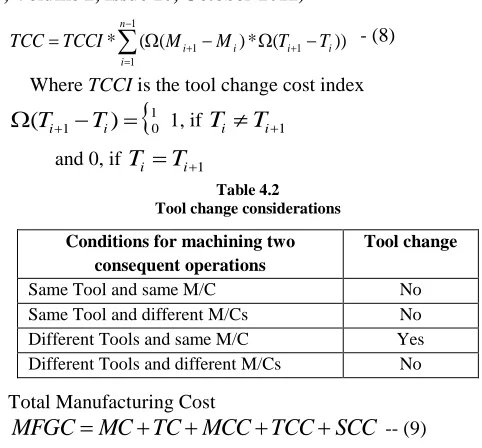
Tool change cost (TCC): A tool change is needed when two adjacent Operations performed on the same machine use different tools.

) ) ( * ) ( ( * 1 1 1 1



         n i i i i

i M T T

M TCCI

TCC

- (8)

Where TCCI is the tool change cost index



1 0

1

)

(









T

_i_₁

Table 4.2 Tool change considerations

Conditions for machining two consequent operations

Tool change

Same Tool and same M/C No

Same Tool and different M/Cs No

Different Tools and same M/C Yes

Different Tools and different M/Cs No

Total Manufacturing Cost

SCC

TCC

MCC

TC

MC

MFGC





-- (9)

These cost factors can be used either individually or collectively as a cost compound based on the requirement and the data availability of the job shop.

Table 4.3

List of machines and usage cost

Machine Type M/c Cost (Rs./min)

M1 Drilling Machine 2

M2 3-Axis Vertical Milling Machine

5

M3 CNC 3-Axis Vertical Milling Machine

12

[image:4.612.49.282.390.655.2]

M4 Boring Machine 6

Table 4.4

List of tools and their usage cost

Tool Type Tool Cost (Rs./min)

T1 Drill 1 0.7

T2 Drill 2 0.5

T3 Drill 3 0.3

T4 Drill 4 0.8

T5 Tapping Tool 0.7

T6 Mill 1 1.0

T7 Mill 2 1.5

T8 Mill 3 3.0

T9 Ream 1.5

[image:4.612.329.559.414.681.2]

(5)

International Journal of Emerging Technology and Advanced Engineering

347

M/c Change Cost Index (MCCI) = Rs. 300

Tool change cost index (TCCI) = Rs. 20 Set-up change cost index (SCCI) = Rs. 90

The shop floor details, various costs and the part details are given as input to the algorithm. The output file contains final pheromone matrix and optimal process plan. After each iteration the pheromone updation and evaporation takes place. If the positional values of each operation are not improving further, then the highest pheromone position is picked for each operation according to precedence constraints and thus the best sequence is generated. The Pheromone matrix is shown for the part 1 in Table 5.9. While applying the Genetic Algorithm for the Process Plan generated by the ACO, there is every chance of changing the positions of the processes, so a Constraint Adjustment Algorithm is used to satisfy all the constraints for each part.

C. Constraint adjustment algorithm

2For initially generated process plan (random sequence) after the crossover and mutation the precedence constraints might not be satisfied. The constraint adjustment algorithm is applied to rearrange the process plan according to the constraints while random properties in it are kept.

1. CASE STUDY

The shop floor details with their cost and the part details are given as input to the algorithm. The output file contains final pheromone matrix and optimal process plan. The pheromone matrix generated for the part 1 is shown in Table 5.9. Here a job shop has been considered; the details are given below.

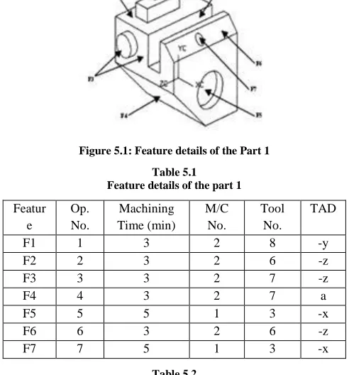
[image:5.612.321.567.171.435.2]

Part 1

Figure 5.1: Feature details of the Part 1 Table 5.1

Feature details of the part 1

Featur e

Op. No.

Machining Time (min)

M/C No.

Tool No.

TAD

F1 1 3 2 8 -y

F2 2 3 2 6 -z

F3 3 3 2 7 -z

F4 4 3 2 7 a

F5 5 5 1 3 -x

F6 6 3 2 6 -z

F7 7 5 1 3 -x

Table 5.2

Precedence constraints between features and operations of the part 1

Feature Oper No.

Precedence constraint description

F1 1 F3 prior to F1.

F3 3 ---

F4 4 F1, F2, F3, F5 & F6 prior to F4

F5 5 ----

(6)

International Journal of Emerging Technology and Advanced Engineering

[image:6.612.48.559.89.716.2]

348

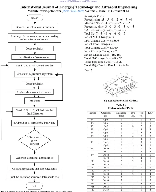
Fig 5.2 Flow Chart of Ant Colony Optimization for Process Planning

Result for Part 1

Process plan 1:3→5→1→2→6→7→4 Machine No: 2→1→2→2→2→1→2 Processing time: 3→5→3→3→3→5→3 TAD:-x→-z→-y→-z→-z→-x→a Tool No: 7→3→8→6→6→3→7 No. of M/C Changes= 3

M/C Change Cost = Rs. 600 No. of Tool Changes = 2 Tool Change Cost = Rs. 40 No. of Set-up Changes = 2 Set-up Change Cost = Rs. 180 Total M/C usage Cost = Rs. 95 Total Tool usage Cost = Rs. 27 Total Mfg Cost for Part 1 = Rs 942/-

Part 2

[image:6.612.52.260.101.707.2]

Fig 5.3: Feature details of Part 2 Table 5.3

Feature details of Part 2

Feature Operation No.

Machining Time

M/c No.

Tool No.

TAD

F1 Op 1 2 1 1 6 F2 Op 2 2 1 1 6 F3 Op 3 4 2 7 5 F4 Op 4 3 2 5 3 F5 Op 5 2 2 5 3 F6 Op 6 3 2 5 3 F7

Op 7 3 1 2 5 Op 8 2 1 3 5 Op 9 2 3 4 5 F8 Op 10 2 1 1 6 F9

Op 11 3 1 2 5 Op 12 2 1 3 5 Op 13 2 3 4 5 F10 Op 14 5 2 5 1 F11 Op 15 2 1 1 6 F12 Op 16 2 1 1 6 F13 Op 17 3 2 5 4 F14 Op 18 4 2 5 4 F15 Op 19 2 1 1 5 F16 Op 20 2 1 1 5 F17 Op 21 5 2 5 4 F18 Op 22 2 1 1 4 F19 Op 23 2 1 1 4

Rearrange the random sequences according to Precedence constraints

Cost calculation

Update pheromone trailvalues

Generate a sequence according to

highest pheromone value If iteration =

given iteration

End

Generate initial random sequences START

Mutation

Yes Initialization of pheromone

Send 90 % of ‗G‘ Global ants for Crossover

Send 10 % of ‗G‘ Global ants for Trail Diffusion Constraintadjustmentalgorithm

Costcalculation

Evaporation of pheromone trail value

No

Constraint checking and cost calculation

(7)

International Journal of Emerging Technology and Advanced Engineering

[image:7.612.53.282.157.536.2] [image:7.612.52.284.157.541.2]

349

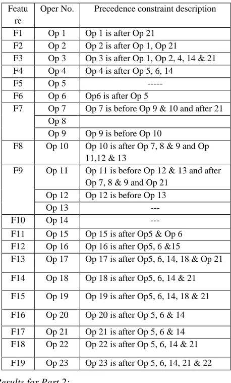
Table 5.4

Precedence constraints between operations of Part 2

Featu re

Oper No. Precedence constraint description

F1 Op 1 Op 1 is after Op 21 F2 Op 2 Op 2 is after Op 1, Op 21

F3 Op 3 Op 3 is after Op 1, Op 2, 4, 14 & 21 F4 Op 4 Op 4 is after Op 5, 6, 14

F5 Op 5 ---

F6 Op 6 Op6 is after Op 5

F7 Op 7 Op 7 is before Op 9 & 10 and after 21 Op 8

Op 9 Op 9 is before Op 10

F8 Op 10 Op 10 is after Op 7, 8 & 9 and Op 11,12 & 13

F9 Op 11 Op 11 is before Op 12 & 13 and after Op 7, 8 & 9 and Op 21

Op 12 Op 12 is before Op 13

Op 13 ---

F10 Op 14 ---

F11 Op 15 Op 15 is after Op5 & Op 6 F12 Op 16 Op 16 is after Op5, 6 &15

F13 Op 17 Op 17 is after Op5, 6, 14, 18 & Op 21

F14 Op 18 Op 18 is after Op5, 6, 14 & 21

F15 Op 19 Op 19 is after Op5, 6, 14, 18 & 21

F16 Op 20 Op 20 is after Op 5, 6 & 14

F17 Op 21 Op 21 is after Op 5, 6 & 14 F18 Op 22 Op 22 is after Op 5, 6, 14 & 21

F19 Op 23 Op 23 is after Op 5, 6, 14, 21 & 22

Results for Part 2:

The two input files containing shop floor details with their cost and example part 3 details have given to the program, the output we will get through output file. It contains final pheromone matrix and generated process plan details.

Process plan 1: 14->5->6->15->16->20->21->22->23->1->2->7->8->9->11->12->13->18->19->17->10->4->3 Machine No: 2->2->2->1->1->1->2->1->1->1->1->1->1->3->1->1->3->2->1->2->1->2->2

Processing time : 5->2->3->2->2->2->5->2->2->2->2->3->2->2->3->2->2->4->2->3->2->3->4

TAD: 1->3->3->6->6->5->4->4->4->6->6->5->5->5->5->5->5->4->5->4->6->3->5

Tool No: 5->5->5->1->1->1->5->1->1->1->1->2->3->4->2->3->4->5->1->5->1->5->7

No. of M/C Changes= 11 M/C Change Cost=Rs. 1650/- No. of Tool Changes= 4 Tool Change Cost=Rs. 80/- No. of Set-up Changes= 5 Set-up Change Cost=Rs. 450/- Total M/C usage Cost=Rs. 249/- Total Tool usage Cost=Rs. 43.5/- Total Mfg Cost for Part 2 = Rs. 2472.5/-

[image:7.612.325.558.211.653.2]

Part 3

Fig 5.4: Feature details of Part 3 Table 5.5

Feature details of part 3

Featu re

Operation No.

Machini ng Time

M/C No.

Tool No.

TAD

F1 Op 1 4 3 7 3

Op 2 1.5 3 6 3

F2 Op 3 3 1 2 6

F3 Op 4 3 3 7 4

Op 5 1 3 6 4

F4 Op 6 2.5 1 3 6

F5 Op 7 2.5 1 3 6

F6 Op 8 4 2 7 7

F7 Op 9 2.5 1 3 6

F8 Op 10 3 3 7 3

Op 11 1 3 6 3

F9 Op 12 5 2 7 3

(8)

International Journal of Emerging Technology and Advanced Engineering

[image:8.612.53.280.153.377.2] [image:8.612.53.284.157.377.2]

350

Table 5.6

Precedence constraints between operations of part 3

Feature Operation No.

F1 Op 1 Op 1 is before Op 2

Op 2

F2 Op 3 ---

Op 5

F4 Op 6 Op 6 is before Op 4 & 5 F5 Op 7 Op 7 is before Op 10 & 11

F6 Op 8 ---

F8 Op 10 Op 10 is before Op 11 Op 11

F9 Op 12 ---

F10 Op 13 ---

The two input files containing shop floor details with their cost and example part 3 details have given to the program, the output we will get through output file. It contains final pheromone matrix and generated process plan details.

Process plan : 7->13->1->9->6->10->12->2->8->3->11->4->5

Machine No: 1->2->3->1->1->3->2->3->2->1->3->3->3 Processing time : 2.5->3.5->4->2.5->2.5->3->5->1.5->4->3->1->3->1

TAD: 6->4->2->6->6->2->2->2->7->6->2->4->4 Tool No: 3->7->7->3->3->7->7->6->7->2->6->7->6 No. of M/C Changes= 9

M/C Change Cost=Rs. 1350/- No. of Tool Changes= 2 Tool Change Cost=Rs. 40/- No. of Set-up Changes= 1 Set-up Change Cost=Rs. 90/- Total M/C usage Cost=Rs. 245.5/- Total Tool usage Cost=Rs. 41/-

Total Mfg Cost for part 3 = Rs. 1306.5/-

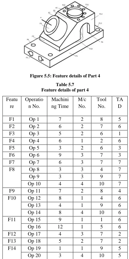
[image:8.612.331.555.158.606.2]

Part 4

Figure 5.5: Feature details of Part 4 Table 5.7

Feature details of part 4

Featu re

Operatio n No.

Machini ng Time

M/c No.

Tool No.

TA D

F1 Op 1 7 2 8 5

F2 Op 2 6 2 7 6

F3 Op 3 5 2 6 1

F4 Op 4 6 1 2 6

F5 Op 5 3 2 6 3

F6 Op 6 9 3 7 3

F7 Op 7 6 3 7 7

F8 Op 8 3 3 4 7

Op 9 3 3 9 7

Op 10 4 4 10 7

F9 Op 11 7 2 8 4

F10 Op 12 8 1 4 6

Op 13 4 1 9 6

Op 14 8 4 10 6

F11 Op 15 9 1 1 6

Op 16 12 1 5 6

F12 Op 17 4 3 7 2

F13 Op 18 5 2 7 2

F14 Op 19 1 1 9 5

(9)

International Journal of Emerging Technology and Advanced Engineering

[image:9.612.64.273.153.496.2] [image:9.612.65.271.157.497.2]

351

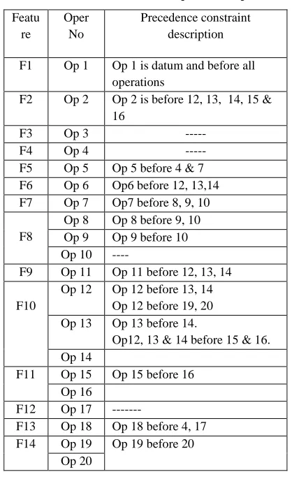
Table 5.8

Precedence constraints between operations of part 4

Featu re

Oper No

F1 Op 1 Op 1 is datum and before all operations

F2 Op 2 Op 2 is before 12, 13, 14, 15 & 16

F3 Op 3 ---

F4 Op 4 ---

F5 Op 5 Op 5 before 4 & 7 F6 Op 6 Op6 before 12, 13,14 F7 Op 7 Op7 before 8, 9, 10

F8

Op 8 Op 8 before 9, 10 Op 9 Op 9 before 10 Op 10 ----

F9 Op 11 Op 11 before 12, 13, 14

F10

Op 12 Op 12 before 13, 14 Op 12 before 19, 20 Op 13 Op 13 before 14.

Op12, 13 & 14 before 15 & 16. Op 14

F11 Op 15 Op 15 before 16 Op 16

F12 Op 17 ---

F13 Op 18 Op 18 before 4, 17 F14 Op 19 Op 19 before 20

Op 20

Process plan 1: 1->3->5->6->2->18->11->12->13->17->7->8->9->19->14->20->10->4->15->16

Machine No: 2->2->2->3->2->2->2->1->1->3->3->3->3->1->4->4->4->1->1->1

Processing time :7->5->3->9->6->5->7->8->4->4->6->3->3->2->8->3-> 4->6->9->12

TAD: 3->1->2->2->6->4->5->6->6->4->7->7->7->3->6->3->7->6->6->6

Tool No:8->6->6->7->7->7->8->4->9->7->7->4->9->9->10->10->10->2->1->5

No. of M/C Changes= 7 M/C Change Cost=Rs. 1050/- No. of Tool Changes= 7 Tool Change Cost=Rs. 140/- No. of Set-up Changes= 7 Set-up Change Cost=Rs. 630/-

Total M/C usage Cost=Rs. 637/- Total Tool usage Cost=Rs. 165/- Total Mfg Cost for Part 4 = Rs. 2622/-

V. PARTICLE SWARM OPTIMIZATION

Particle swarm optimization (PSO) is a popular problem solving technique in the swarm intelligence (SI) paradigm. It was first introduced by Kennedy and Eberhart in 1995. PSO is used to optimize continuous nonlinear mathematical functions by borrowing ideas from the swarms such as flocks of birds and schools of fish searching for food. PSO evolves solutions based on individual experience and group experience, rather than using evolutionary operators. The job shop scheduling problem is solved to minimize the make span.

In this paper we use the global model equations as follows (Shi & Elbert, 1999):

  



 





1

2

id id id id

gd id

V

W V

C

Rand

p

X

C

rand

p

X

 













 

1 and

id id id

X X V

 

2

where

V

_id is called the velocity for particle I, represents the distance to be traveled by this particle from its current position,

X

_id represents the particle position,

p

_idwhich is also called as pbest (local best solution), represents ith particles best previous position, and

p

_gd, which is also called gbest (global best solution), represents the best position among all particles in the swarm. W is the inertial weight. It regulates the trade-off between the global exploration and local exploitation abilities of the swarm. C1 and C2 represent the weight of the stochastic acceleration terms that pull each particle toward pbest and

gbest positions.

Rand

 

and

rand

 

are two random functions in the range [0,1].

The inertia weight is set using the following equation

max min

max

max ,

W W

W W iter

iter

  

Where max

W

= initial value of the weighting coefficient

min

W

= final value of the weighting coefficient

max

(10)

International Journal of Emerging Technology and Advanced Engineering

352

A. Particle position and velocity initialization and

limitation

Begin

Step 1. Initialization

Initialize parameters, including swarm size, maximum of generation, Wmax, Wmin, C1, C2;

Step 2. Assignment and scheduling Generation=0;

Initialize particle‘s position and velocity stochastically;

Evaluate each particle‘s fitness;

Initialize gbest position with the particle with the lowest fitness in the swarm;

Initialize pbest position with a copy of particle it self;

While (the maximum of generation is not met) Do {

generation = generation+1;

Generate next swarm by equations;

Evaluate swarm {

Compute each particle‘s fitness;

Find new gbest and pbest by comparison;

Update gbest of the swarm and

pbest of each particle; }

}

Step 3. Output optimization results. End.

C. Particle representation (encoding): based on operation and particle position sequence

As PSO is used to optimize the problem, one key issue is the encoding, which is called particle representation in this paper. Suitable particle representation should importantly impact the optimization result and performance of PSO. In most applications of PSO, it is applied to the continuous optimization problems. In these optimization problems, particle position xi is directly denoted as the solution, which is continuous value. Velocity vi, acceleration

continuous constants.

PSO completes the searching process in the continuous space that limits the use of PSO in the discrete space or combination optimization problem. However, job shop scheduling problem is a combination optimization problem, and it‘s feasible solutions are the sequence of operations of all jobs.

D. PSO for FJSP

The feasible solution of JSP is the operation sequence of all jobs. For the particle position xi = (xi1, xi2 ,… xij,…, xid) , all position vectors xij(the total number is equal to d) also have a sequence (increasing sequence or decreasing sequence). So the operation sequence of all jobs and the sequence of the particle position vectors can be linked together, and the mapping is gained between the scheduling solution and the particle position.

In the mapping between the particle and the scheduling solution is established through connecting the operation sequence of all the jobs with the particle position sequence. Each operation in the operation sequence of all the jobs is assigned on each machine in turn to form the scheduling solution.

(11)

International Journal of Emerging Technology and Advanced Engineering

[image:11.612.61.238.113.494.2]

353

Fig 6.1 Particle Swarm Optimization Flow Chart

Let:

J= {1, 2... n} denotes the set of jobs; M= {1, 2… m} denotes the set of machines;

N= {0, 1, 2… n+1} denotes the set of operations, where 0 and n+1 represents the dummy start and finish operations, respectively.

Here a set J of n jobs are to be processed on a set M of m machines. Each job j consists of a sequence of nj operations

(routing) i.e. Oj,1, Oj,2, … Oj,,nj. The execution of each

operation i of a job j (Oj,i) requires one machine out of a set

of given machines called Mj,i M.

[image:11.612.341.543.144.341.2]

The results of PSO based optimization heuristic are compared against the results of the benchmark problems in Table 6.1.

Fig 6.2: The mapping, decoding and updating of the particle

E. Assumptions made in this work

 No two operations of the same job may be processed simultaneously.

 No Pre-emption

 Processing the job twice on the same machine is not allowed.

 Setup times of machines and move time between operations are negligible.

 No machine may process more than one operation at a time.

 The number of jobs is known and fixed.

 The number of machines is known and fixed.

 The processing times are known and fixed.

The Process Planning results obtained from the ACO are used as the input for the JSP and the results obtained are given below.

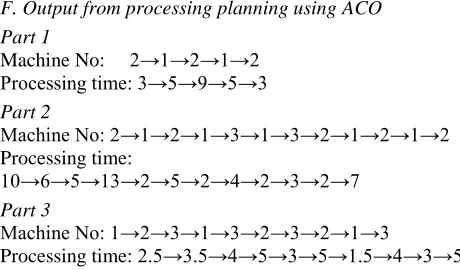
F. Output from processing planning using ACO

Part 1

Machine No: 2→1→2→1→2 Processing time: 3→5→9→5→3

Part 2

Machine No: 2→1→2→1→3→1→3→2→1→2→1→2 Processing time:

10→6→5→13→2→5→2→4→2→3→2→7

Part 3

Machine No: 1→2→3→1→3→2→3→2→1→3

Processing time: 2.5→3.5→4→5→3→5→1.5→4→3→5 Start

Initialize particles with random position and velocities

Apply Local Search

Compare / Update fitness value with P Best and G Best

EvaluateFitness

Meet stopping Criterion

Update velocity and position

[image:11.612.324.554.565.700.2]

(12)

International Journal of Emerging Technology and Advanced Engineering

354

Part 4

Machine No: 2→3→2→1→3→1→4→1

Processing time: 15→9→18→12→16→2→15→27

VI. RESULT

The resultant schedule generated using the particle swarm for the above products is

For 1000 iterations and swarm size 48

No of Jobs: 4 No of Machines: 12 No of Operations: 48 No of Particles in swarm: 48 Max No of iterations: 1000

The PSO algorithm using the above encoding procedure is developed and tested for the FJSP and the results obtained after 200 iterations are as follows.

Gbest sequence is

4→1→2→1→4→3→4→2→3→2→4→3→2→4→1→2 →3→3→4→2→3→4→1→2→2→1→4→3→2→2→1→ 3→2→3→3→4→4→1→1→1→4→3→3→1→1→1→ 4 Gbest=130

Optimum Process Time with 1000 Iterations & Swarm Size 48: 130

VII. CONCLUSIONS

Since the generation of various feasible plans and to find the best among them constitutes an NP-hard complete combinatorial problem. Hence an efficient heuristic search is required to solve such problem. We applied the ACO algorithm to solve the problem of generating optimal process plan for a given part. The approach models process planning considering the machine, tool, and tool approach directions for each operation. Precedence relationships among all the operations required for a given part are used as the constraints for the solution space. The optimal process plan is found based on the minimum total cost criteria.

The Particle Swarm Optimization algorithm is used to solve FJSP problems since the experimental results show that PSO for JSP is very effective, and can find the best known solution for the cited benchmark instances.

On identifying the need to integrate the process planning and the scheduling, the output obtained through ACO is taken as the input to the Scheduling and the optimal makespan is obtained for the FJSP Problem considered. Thus, the minimum makespan for the given JSP is obtained at the minimum possible cost.

REFERENCES

[1 ] Chandrasekharan Rajendran, Hans Ziegler, 2004, ―Ant Colony

Algorithms For permutation Flow Shop Scheduling to minimize makespan/total flow time of jobs.‖ European Journal of Operational Research 155 pp. 426-438.

[2 ] Cheng, Wang 1999, ―A Note on Two-Machine Flexible

Manufacturing Cell Scheduling‖, IEEE Transactions on Robotics and Automation, 15, 1, 187–190.

[3 ] Christos H. Papadimitriou, Paris C. K, 1980, ―Flow shop Scheduling with Limited Temporary Storage‖, Journal of the Association for Computing Machinery, Vol. 27. No. 3, pp 533-549.

[4 ] Colorni A., Dorigo M., & Maniezzo V., 1991, ―Distributed optimization by ant colonies‖. In the Proceedings of ECAL 91 — European Conference on Artificial Life, pp. 134-142, Paris, France: Elsevier, Amsterdam.

[5 ] Dorigo M., & Gambardella, L. M., 1997, ―Ant colony system: a cooperative learning approach to the Traveling Salesman Problem.‖ IEEE Transactions on Evolutionary Computation, 1997 (1), 53– 66. [6 ] Dorigo M, Maniezzo V., & Colorni, A., 1996, ―The ant system:

optimization by a colony of cooperating agents.‖ IEEE Transactions on Systems, Man & Cybernetics B, 26(2), 29– 41.

[7 ] Gambardella, L. M., Taillard, E., & Dorigo, M., 1997, ―Ant colonies for QAP.‖ IDSIA, Lugano, Switzerland, Technical Report IDSIA 97-4.

[8 ] [8] Gupta, E. A. Tunc 1994, ―Scheduling a Two-Stage Hybrid Flow shop with Separable Setup and Removal Times‖, European Journal of Operational Research, 77, 3, 415–428.

[9 ] Hans Rock, 1984, ―The Three-Machine No-Wait Flow Shop Is

NP-Complete‖ Journal of the Association for Computing Machinery, Vol. 31, No 2, pp 336-345.

[10 ]Jayaraman V.K, B.D. Kulkarni, 2000, ―Ant colony framework for optimal design and scheduling of batch plants‖, Computers and Chemical Engineering, vol. 24, pp.1901-1912.

[11 ]Johnson, S. M. 1954, ―Optimal Two- and Three-Stage Production Schedules with Setup Times Included‖, Naval Research Logistics Quarterly, 1, 1, 61–68.

[12 ]Niem-Trung L. Tra, 2000, ―Comparison of Scheduling Algorithms for a Multi-Product Batch-Chemical Plant with a Generalized Serial Network‖, MS Thesis, The Virginia Polytechnic Institute and State University, Blacksburg, Virginia.

[13 ]Stutzle T, 1998, ― An ant approach for the flow shop problem‖, In fifth European Congress on Intelligent Techniques Soft Computing, vol. 3, Verlag Mainz, pp. 1560-1564,.

[14 ]Xiao-Rong Wang, Tie-Jun Wu, 2003, ―An Ant Colony Optimization

Approach for No-Wait Flow Line Batch Scheduling with limited Batch size.‖, Proceedings of the 42nd_{IEEE conference on Decision}