A Simulation Based Method for Teaching Reference Frames in Secondary Schools

A Simulation Based Method for Teaching Reference

Frames in Secondary Schools

Tünde Tóthné Juhász1,2,*_{, András Juhász}3_{, Zsolt Szigetlaki}4

1_{Karinthy Frigyes High School, Hungary}

2_{Physics Education PhD Program, Eötvös University, Hungary} 3_{Department of Material Physics, Eötvös Loránd University, Hungary}

4_{Intellisense Zrt., Hungary}

Copyright©2017 by authors, all rights reserved. Authors agree that this article remains permanently open access under the terms of the Creative Commons Attribution License 4.0 International License

Abstract

taught at an early stage of secondary school physics is quite challenging for students. The two main reasons behind this are the high level of abstraction required and the lack of understanding of the vector nature of velocity. In the paper we introduce a method we use successfully in teaching reference frames with our students and which is based on computer simulations. We use a new simulation program, called Fizika, which is developed by a Hungarian team and is available for all science teachers for free. Through the simulations and graphs of motions, we investigate different stationary and uniformly moving reference frames and introduce the concept of relative velocity. With the help of the simulations we can provide our students experimental experience, on which they can build with much more confidence and which will lead them to a deeper understanding. The simulations can also be used for extracurricular lessons with talented students, since the program can also be used to investigate complex motions and their graphs.

Keywords

Velocity, Galilean Transformation, Teaching Methods

1. Introduction

Teaching reference systems in secondary school doesn’t seem to be a very difficult task at first. Most students learn the basic definitions (origin, reference frame, relative speed) superficially, but very few of them get to deeper understanding. The reason behind this is mainly that students stick to their own approach that comes from their everyday experiences and so they use the scalar concept of speed instead of the vector concept of velocity, which leads to certain problems even in easy situations such as uniform motions. One such misunderstanding of vectors is when

students think that deceleration is always a negative acceleration [1].

The concept of reference frames should be introduced gradually, so we usually start by changing between stationary reference frames, which students understand quite quickly. The next step is then to change from a stationary to a uniformly moving reference frame. An example of such a situation is when the motion of an object is observed from a moving car or train.

Galileo was the first to deal with the problem of reference frames and he generalized his observations in the so called Galilean relativity, which basically states that there is no experiment that can distinguish between a stationary and a uniformly moving system. This concept leads to the field of dynamics as well as the concept of uniformly accelerating reference frames, but the latter is too complex to be taught to an average student in secondary school.

Teachers around the world want their students to understand and not only learn physics, so in the following paper we will first summarize the problems our students usually encounter with the concept of reference frames and then offer a possible solution, which is based on a simulation software called Fizika, which was developed by a Hungarian team, and is available worldwide in English. This program can be used both to help students who find physics a challenge and also to give challenging problems for talented students. This versatility of the software will be demonstrated by examples from our own teaching experience.

2. Problems That Students Have in

Understanding Reference Frames

1. The first problem is that reference frames are not used in our everyday life, therefore require such an amount of abstraction that is hard to understand at the age of 14-15. Furthermore, this topic is based on graphical representation, which again is very abstract. (A typical problem that shows how hard it is to distinguish between different graphs is the case of the path of oblique projection and the position-time graph of a vertical projection. These two often get mixed up by students.) So we get into the trap of trying to explain an abstract concept with another abstract concept, and that doesn’t work well. The only solution to this problem is if these things are taught gradually and with a lot of examples and exercises that help the students gain a deeper understanding. (This is where using software Fizika gives an enormous help.)

2. The second problem is that small children all have a natural reference frame, in which they are at the origin, and gradually they get used to this fact. In physics, however, when we need to measure positions and velocities, we need to find an origin (usually stationary), from which every distance is measured. Most of the students understand this easily, but when it comes to changing from one reference frame to another, they get uncertain about what to do. Thus it’s essential to make students solve problems in which the original reference frame is changed to another (also stationary) frame. This way they should think about the changes such a step causes in the graphs of the motion - mainly that position changes, but velocity remains the same. Computer simulations in which the origin of the system can be repositioned (as in Fizika) are perfect for giving the students ample experience about this.

3. The third and most important problem arises when we start to teach moving reference frames in secondary school. It is a hard topic even though students have everyday experiences about it. They had all once been struck by the recognition that trees and houses seem to move backwards when they travel in a car. They also know that when we sit in a car moving fast, another car overtaking us seems to move surprisingly slowly, and cars coming from the opposite direction seem to move strikingly fast. However, human mind can’t easily perceive relative speeds and this leads to a high number of overtaking accidents. The reason behind these accidents usually originates from the difficulty to estimate the relative speeds of other cars (the one to be overtaken and the one coming opposite) and thus guess the distance needed to complete the manoeuvre safely. Investigating an overtaking situation from both stationary and moving reference frames is a very edifying experience for students. Apart from helping to solve the above problems, Fizika

software can also be used with talented students. There are problems, where the solution gets simplified if the whole situation is observed from a moving reference frame. Thus investigating motions and analysing their graphs from stationary and moving reference frames is an essential task to be given to talented students. Unfortunately time for teaching physics is tight and doesn’t always allow for deep studies, however, with the help of a simulation program that both visualizes the motion of objects and draws their graphs at the same time, we can complete this task very effectively.

In the following sections we will first introduce the simulation program used (Fizika) shortly, then show simulations we made and used in our classes. These simulations were designed to lead our students through the topic of reference frames with a detailed and step-by-step method (starting from the easiest and finishing with the hardest problems) that enabled them to gather experience through experimenting.

3. A Short Introduction to Software

FIZIKA

Fizika software is a newly developed educational simulation software developed by Hungarian team, called Intellisense Zrt., whose other well-known product is LabCamera that is included in Intel computers [2].

These kinds of software are offered for free use for all science teachers in the world as part of the “Intelligence for Science Teachers” Programme (IST). This program was called to life by the developers to build and support a community of passionate science teachers through creating and sharing exciting science education materials free of charge. As well as offering free download of the software [3], IST also provides downloadable materials such as lesson plans and videos for registered members. Teaching experiments have already been run to investigate the effectiveness of the programs and their outcomes were positive. [4]

Obviously, there are other software that could be used for the same purpose (such as Algodoo) quite as successfully as Fizika. However, Fizika has the advantage of being simple enough to let teachers get acquainted with it in less than an hour and at the same time is complex enough to offer a wide variety of simulations and options. Furthermore, teachers are offered ready-made simulations with lesson plans, and this comes very useful, especially for those, who don’t have the time or talent to develop their own simulations.

parameters of every element are variable, such as mass, coefficient of friction, elasticity. When the simulation is started, the program takes these variable parameters as well as some constants (free-fall acceleration) into account and solves the differential equations of motion of every element numerically. The solution is visualized on the screen and allows the user to observe the motion of the elements.

If a virtual marker or sensor is fixed to a given object, the program automatically draws the graph of either the horizontal or vertical component of its motion (position-time, velocity-time or acceleration-time graph).

The origin of the reference system is automatically set to the middle of the screen, but can be repositioned to another point or even be fixed to a moving object. All positions and velocities will then be measured from this point. Therefore the program allows users to observe motions from uniformly moving or even accelerating reference frames.

The fact that the program offers graphical representation of motions is an immense help in teaching graphs and their relationships with each other, while repositioning the origin is an essential tool in teaching reference frames.

The simulation program can also be used in the topic of dynamics, where vector representation of forces is a powerful tool to make students understand the basic concepts of forces.

4. Set of Simulations for Teaching

Reference Frames

The simulations shown below are for teaching reference frames. Although the program would enable us to handle accelerating frames as well, we restricted the topic to secondary school syllabus, therefore only stationary and uniformly moving frames will be discussed here. All simulations are available on the internet [5].

4.1. Investigating the Role of the Origin

It’s essential to spend a little time on the role of origin when we start teaching graphs of motion. This is needed, because many students nurture a false theory that all position-time graphs must start at the origin. Obviously talented students have no problem in imagining how the choice of origin affects the graph of motion, but for an average student it is a challenging question. Therefore it is much better to show a simulation experiment that can be investigated and played with than to only explain verbally and expect students to understand.

Simulation “refframe 1” shows a car moving to the right with a constant velocity of . The motion of the car is observed by several people (A, B, C, D, E and F) who are at a distance of from each other (Fig. 1). The task given to students is to observe and analyse position-time and velocity-time graphs of the car, seen from the positions

of different people.

Figure 1. Simulation “refframe 1”, in which the uniform motion of a car is observed from different stationary reference frames.

Students are asked to run the simulation several times, resetting the origin to a different person and rerunning it each time.

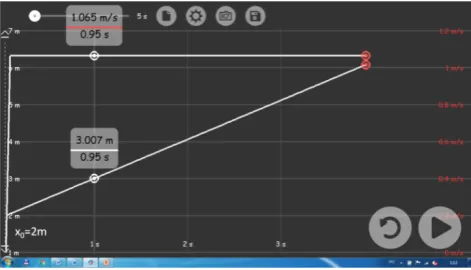
The simulation is designed so that the car always starts to move from in front of the third observer (C). It is best to start the investigation at the left end of the observers (at A). In this case the position-time graph of the car - that is a straight line with a positive slope of - will not start at the origin, but at (Fig.2). The velocity-time graph of the car is a horizontal straight line showing constant velocity.

Figure 2. Graphs of the uniform motion of the car as seen by observer A. The velocity-time graph is a horizontal straight line, the position-time graph is a sloping straight line that starts at x0=2m.

The first task after making the program draw the graphs is to discuss why the position-time graph starts at x0=2m,

because this is what emphasises that position-time graphs do not necessarily go through the origin. Then it’s also possible to determine the velocity of the car and check that it’s really v=+1ms-1_{. This can be done either by reading the}

value of the velocity-time graph or by determining the slope of the position-time graph.

After analyzing the first graphs, we should ask the students to find the observer, from whose point of view the car will start its motion from the origin. Most students find the answer (C) easily, but it’s useful to check it by rerunning the simulation after repositioning the origin to observer C.

1

1ms− m

1

1

1_ms− m

It’s useful to compare the two graphs obtained so far (Fig. 3).

Figure 3. Simulation “refframe 1”. Graphs of the car from the point of view of observer C (left) and A (right). The initial positions are x0=0m and

x0=2m respectively.

At first sight the two graphs look identical, although the two position-time graphs start from different points. This is because of the design of the program: for optimizing the size of a graph, the program scales and shifts the axes so that the graph will be big enough to be investigated. Students should be made aware of this and at the same time it’s useful to draw the two graphs in one coordinate system to show that the two position-time graphs are shifted along the vertical axis with respect to each other.

The velocity of the car is the same in both cases: v=+1ms-1_{. This can be verified by either reading the values}

from the v-t graph or calculating the slope of the x-t graphs. Analysing the motion of the car from different points clarifies that the graph of a motion is dependent on the position of origin. The investigation of the simulation can be finished as homework: three more graphs are given, which are graphs of the same car from the views of different observers. The task is to identify the observer for each graph by analysing the initial position.

4.2. Negative Velocity

If students have managed to understand that position-time graphs do not always pass through the origin, the next problematic point – that velocity can be negative - should be handled.

The problem stems from the fact that in our everyday life the concept of speed is used, which is a scalar quantity and therefore doesn’t express direction. However, in physics the concept of velocity is used most of the time, and therefore direction has an important role.

The fact, that kinematics starts with the investigation of motions along a straight line (1 dimension), makes the situation even worse. Students quickly get used to the idea of a velocity that is represented by a number (no direction shown) and for simplicity we almost always assume that objects move in the positive direction, thus we use a positive number for representing velocity. This obscures the idea of direction, which can still be emphasised in 1 dimension: in this case the direction of the velocity is given by a positive or negative sign. Thus it’s important to investigate situations in which the velocity takes a negative value, in order to emphasise the concept of vectors for students.

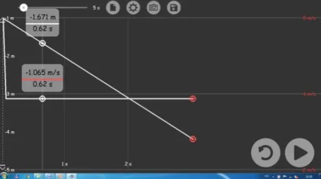
One such situation is shown by simulation “refframe 2”, which is almost the same as “refframe 1”, but in this case the car moves towards the left, therefore its velocity will be

v=-1ms-1_{. In case of primary school students, the}

simulation can be used and worked through exactly the same way as shown in the previous case, but in case of secondary school students it’s enough to investigate the graph of the car from the point of view of only one observer. The negative value of velocity can either be read from the v-t graph directly or can be calculated from the slope of the x-t graph.

Figure 4. Simulation “refframe 2”. The car moves to the left, therefore its velocity is negative.

Investigating this simulation takes only 10 minutes, but it has an extremely important role in emphasizing that velocity is a vector quantity.

4.3. Changing from Stationary to Uniformly Moving Reference Frame

Figure 5. Simulation “refframe 3”. Changing from a stationary to a moving reference frame.

The task in this case is to investigate the graphs of the two objects from a stationary then from a uniformly moving reference frame (from the frame of the car). Initially the origin is fixed to the ground below the car. If the simulation is started, the graphs shown in Fig. 6 will be obtained.

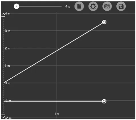
Figure 6. The position-time graphs of the house (horizontal line) and car observed from a stationary reference frame in simulation “refframe 3”.

It can be read from the graphs that the position of the house remains x=-1m (horizontal line), while the car starts from the origin and moves with a constant speed of vcar=+2ms-1 to the right (straight line with positive slope).

Let’s fix the origin to the car now, and rerun the simulation. The new graphs obtained are shown in Fig. 7.

Figure 7. The position-time graphs of the house and car observed from a moving reference frame (fixed to the car) in simulation “refframe 3”.

The graph shows that the car is stationary in its own reference frame, since its graph is a horizontal line having a constant value of xcar=0m, while the house seems to move

backwards (towards the left) with a velocity of vhouse=-2ms-1.

It’s also useful to investigate the velocity-time graphs of the objects in the two different reference frames. These are shown in Fig. 8.

Figure 8. Velocity-time graphs of the house and car observed from a stationary (left) moving reference frame (right) in simulation “refframe 3”.

4.4. Relative Velocity of Cars Moving in the Same Direction

In the previous simulation the motion of stationary objects were investigated from a moving reference frame. The next step is to investigate the motion of moving objects from a moving reference frame.

When the concept of relative speed is taught in secondary schools, we ask students to remember and build on their experiences of seeing other cars move from their own moving car. As I mentioned before, the perception of relative speed is a difficult task for the human brain, therefore it is much better to investigate a simulation as well and to show experimental results verifying our memories.

In simulation “relspeed 1” two cars moving in the same direction with different speeds are modelled by two boxes as shown in Fig. 9.

Figure 9. Screenshot of simulation “relspeed 1”. The faster car (A) overtakes the slower one (B), which has a head start of 2m.

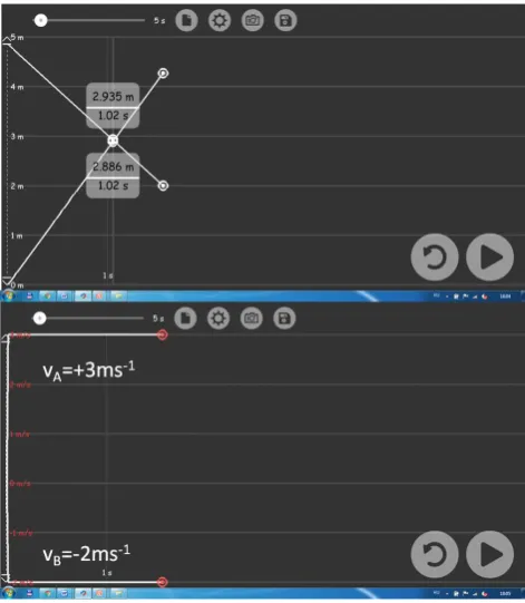
First the graphs of the cars should be drawn in a stationary reference frame. The origin is fixed to the ground below the faster car (A). The faster and slower cars have a velocity of vA=+3ms-1 and vB=+2ms-1 respectively

and the initial distance between them is 2m. If the simulation is started, the markers on both cars measure position, thus the program automatically draws the position-time graphs. With a simple click this graph can be changed to velocity-time graphs as well (Fig. 10).

The upper graph shows the time and position where the cars meet: it takes 2s for the faster car to reach the slower one.

Let’s fix the origin now to car B and discuss the expected outcome with the students. Then restart the simulation and investigate the position-time and velocity-time graphs obtained in the moving reference frame (Fig. 11).

Figure 10. Simulation “relspeed 1”. Position-time (top) and velocity-time (bottom) graphs of the two cars in a stationary reference frame.

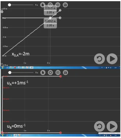
These new graphs show that car B remains in the origin in its own system throughout the motion, thus its graphs are constant zero functions. Car A has an initial position of -2m, which means that initially it is at a distance of 2m to the left from car B.

Car A moves towards to origin at a constant velocity, the time needed to reach it can be read from the graph (2s). The velocity of car A in the reference frame of car B is less, uA=+1ms-1.

This verifies our expectation that in case of two cars moving in the same direction, relative speed can be calculated as the difference of the two speeds. With average students this is the point, where we end the investigation, but with talented students we can continue with the following analysis.

When we change from stationary to a moving reference frame, the velocity of an object in the new frame can be calculated by subtracting the velocity of the frame from the original velocity (measured in stationary frame) of the object:

(1) where v and u represent the velocities measured in stationary and moving reference frames respectively.

Since the velocities in the stationary reference frame were vA=+3ms-1, vB=+2ms-1, the velocity of car A in the

system fixed to car B should be

, which is the result we got in the simulation as well.

Equation (1) is a general formula that works for all cases. As a quick check, we can relate back to simulation “refframe 3”, where the velocity of the house can be calculated in the reference frame of the moving car as:

, which was really the result obtained in that simulation.

It’s similarly easy to show that if we return back to simulation “relspeed 1” and fix the reference frame to car A, the relative velocity of car B will be:

, thus car B will seem to move to the left with respect to car A. The graphs obtained in this case are shown in Fig. 12:

Figure 12. Simulation “relspeed 1”. Position-time (top) and velocity-time (bottom) graphs of the two cars in uniformly moving reference frame, fixed to car A.

4.5. Relative Velocity of Cars Moving in the Opposite Direction

In simulation “relspeed 2” cars (which are modelled by rectangles again) move in opposite directions. The tasks are exactly the same as in case of “relspeed 1”: the graphs of the cars should be investigated first in a stationary, then in a moving reference frame (fixed to one of the cars).

Figure 13. Screenshot of simulation “relspeed 2”. Two cars move in opposite directions.

frame object

object v v

u = −

1 1

1 _{2 1}

3 − − − = −

= −

=v v ms ms ms

u_{A A B}

1 1

1 _{2 2}

0 − ₋ − ₌₋ −

= −

=v v ms ms ms

u_{house house car}

1 1

1 _{3 1}

2 − − − =− −

= −

=v v ms ms ms

Initially the origin is fixed to the ground below car A. The velocities of the cars are vA=+3ms-1 and vB=-2ms-1 ,

where the negative sign of vB shows that car B moves in the negative direction (to the left). The initial distance between the cars is 5m. If the simulation is started, the markers on both cars measure position, thus the program automatically draws the position-time graphs. With a simple click this graph can be changed to velocity-time graphs as well (Fig. 14).

Figure 14. Simulation “relspeed 2”. Position-time (top) and velocity-time (bottom) graphs of two cars moving in opposite directions in a stationary reference frame.

The position-time graph shows that the cars meet after 1s.

Let’s fix the origin now to car A, then restart the simulation and investigate the position-time and velocity-time graphs obtained in the moving reference frame (Fig. 15).

These new graphs show that car A remains in the origin in its own system throughout the motion, thus its graphs are constant zero functions.

Car B moves towards to origin at a constant velocity, the time needed to reach it can be read from the graph (t=1s). The velocity of car B in the reference frame of car A is now

uB=-5ms-1.

This verifies our expectation that in case of two cars moving in the opposite direction, relative speed can be calculated as the sum of the two speeds.

In case of talented students further analysis can be carried out again to check the validity of (1).

Since the velocities in the stationary reference frame were vA=+3ms-1, vB=-2ms-1, the velocity of car B in the

system fixed to car A should be

Figure 15. Simulation “relspeed 2”. Position-time (top) and velocity-time (bottom) graphs of the two cars in a uniformly moving reference frame, fixed to car A.

, which is the result we got in the simulation as well. It’s similarly easy to show that if the reference frame is fixed to car B, car A will have a relative velocity of +5ms-1_.

The general validity of (1) is of great importance: a vector equation can be applied to all cases and it’s the direction of the velocity vectors that will decide whether the magnitude of the relative velocity is the sum or the difference of the original magnitudes of velocities. 4.6. Simulation of an Overtaking

The simulations shown in the previous subsections help students understand the concept of reference frames taking one step at a time. The simulation program, however, offers more than that: it can also be used for modelling more complex problems, therefore its use is not restricted to ‘average’ students, but widens to talented ones as well.

The problem discussed here is an overtaking. Investigating this situation is a good occasion to summarize and review the topic of reference frames, since it contains motions in both the same and the opposite directions. I would also like to point out that modelling is a task that is not trivial for secondary school students, however, it can be used successfully with talented ones.

4.6.1. Problem

A car moving with a constant speed of 90kmh-1

1 1

1 _{3 5}

2 − ₋ − ₌₋ −

− = −

=v v ms ms ms

overtakes a 18m long lorry moving at 80kmh-1_{. The car}

starts and ends the manoeuvre keeping a safety distance of 15m between the two vehicles. Find the time taken by the car to overtake the lorry.

4.6.2. Solution Based on Theoretical Calculations

First let’s change the speeds to SI units: vcar=25ms-1,

vlorry≈22ms-1. Although safety regulations say that a

distance covered in 2s should be kept between vehicles (which in our case would be 50m), this is rarely the case when we start an overtaking maneuvre. Thus it is more realistic to assume that the distance kept between the vehicles is 15m both before and after the overtaking. The car can be assumed to be point-like, since this 15m allows for the length of the car as well.

If the situation is observed in a stationary reference frame, the equation for the overtaking would be:

, (2) where t is the time taken for the overtaking. Solving the equation for t gives t=16s. During this time the car covers a distance of 400m.

The same result can be obtained by using a reference frame fixed to the lorry. In this frame the car needs to cover a distance of 48m (twice the safety distance plus the length of the lorry) and moves with a relative speed of 3ms-1_{, thus}

it takes t=48/3=16 seconds to overtake the lorry.

Note: if there is traffic in the opposite direction as well, we need to know the minimum distance at which a car must be in the other lane in order to avoid accident. Assuming that the car in the opposite direction moves with 90kmh-1_=25ms-1 _{as well, its relative speed with respect to}

the overtaking car would be 50ms-1_{. This means that}

calculating with the critical 16s, we get that the minimum distance between the two cars should be 800m.

This considerably big distance shows that in order to complete an overtaking at such high speeds, we need a long, clearly visible space in the opposite lane. Furthermore, this minimum distance in the opposite lane increases if the relative speed of the car with respect to the lorry decreases. This suggests that in order to complete a safe overtaking, the relative speed between the vehicles should be big enough. However, increasing relative speed to finish a risky overtaking is not always the good solution: although the time needed to finish the manoeuvre decreases, the relative speed of the car coming from the opposite direction increases. Thus in most of the cases it’s safer to decelerate and return back behind the vehicle that was to be overtaken.

It’s useful to check our calculations by a quick simulation.

4.6.3. Solution Based on Simulation

Simulation “overtaking” models the problem solved above. It is impossible to give a length of 18m to a lorry in the program, therefore the lengths should be re-scaled:

every length will be reduced to 1/100 of its real value. Then the question arises naturally: what else should be re-scaled to get a realistic result? This is a question, which is not trivial to answer for secondary school students. First we need to decide what we want to keep realistic: in this case it’s naturally the time. Since t=s/v, it’s clear that we need to re-scale speeds: they should also be reduced to 1/100 of their real values. Once our model is set up, all we need to do is draw the simulation.

In the simulation (see Fig. 16) an orange rectangle (of length 0.18m) models the lorry and two red rectangles (both 0.15m long) model the safety distance before and after the lorry. The car moves on a separate lane (to avoid collision) above the lorry. The length of the car is only 0.04, thus it seems point-like.

Figure 16. Screenshot of simulation “overtaking”. Lorry is modelled by an orange rectangle, and car is point-like and moves above the lorry.

The car and lorry have a constant speed of 0.25ms-1 _and

0.22ms-1 _{respectively, which are 1/100 of their real speeds.}

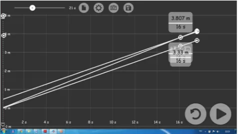
Virtual markers are fixed to the car and to the front of the first and back of the rear red rectangle. The position-time graphs obtained in a stationary reference frame (origin is fixed to the ground) are shown in Fig. 17.

Figure 17. Position-time graph of the overtaking measured in a stationary reference frame.

Apart from finding the time needed for the overtaking (t≈16s), it is also possible to find the approximate distance moved by the car during the overtaking. The value read

t v t v_lorry⋅ = _car⋅ +

+

+18 15

from the graph is about 3.8m, which should be multiplied by 100 to get the real value of 380m≈400m.

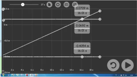
In order to review the concept of reference frames, it’s advised to re-run the simulation after fixing the origin to the front of the first red rectangle. In this case the car will finish the overtaking manoeuvre when it reaches the origin.

Figure 18. Position-time graph of the overtaking measured in a uniformly moving reference frame (fixed to the lorry).

Apart from reading the time taken (t≈16s), it is also possible to determine the relative speed of the car, which is the slope of the line, approximately 0.03ms-1_{, which}

corresponds to a real value of 3ms-1_.

This problem is a good summary of the topic of reference frames, since it contains motions in both the same and opposite directions.

5. Conclusions

The set of simulations discussed above guides secondary school students through the topic of reference systems in such a way that allows for experimenting and discovering the critical points (e.g. relative speed) in an individual way. This way students can build on their own experimental experiences and results instead of learning theory without deeper understanding. The above simulations are designed for 14+ years old students, therefore can be used

successfully in secondary schools.

It’s also shown that simulation program Fizika can be used with talented students as well for solving and modelling more complex tasks.

It should be kept in mind that the program has certain limitations (it’s not possible to know the error of a measurement) and therefore cannot be used for higher academic studies and handled as a professional simulation software such as e.g. Dynamic Solver.

However, since the program can be downloaded free and there are many teaching materials (lesson plans and ready-made simulations) available, Fizika is still a powerful tool for making our physics classes interesting and effective.

Acknowledgements

This study was funded by the Content Pedagogy Research Program of the Hungarian Academy of Sciences.

We would like to express our gratitude to Intellisense Zrt. for sharing their software with us and with all science teachers for free.

REFERENCES

[1] https://in.answers.yahoo.com/question/index?qid=1006042 820943 (visited 06.11.2016)

[2] http://intellisense.education/home/ (visited 06.11.2016) [3] http://intellisense.education/home/index.php?register=teach

er (visited 06.11.2016)

[4] Tóthné Juhász, T., A computer simulation based teaching experiment, Teaching Physics Innovatively Conference (Budapest, 2015), p249-254. Available at http://csodafizika.hu/fiztan/letolt/konfkotet2015.pdf