THE PERFORMANCE EVALUATION OF DIFFERENT LOGICAL TOPOLOGIES AND THEIR RESPECTIVE PROTOCOLS FOR WIRELESS
SENSOR NETWORKS
NAYEF ABDULWAHAB MOHAMMED ALDUAIS
A project thesis submitted in
fulfillment of the requirement for the award of the Degree of Master of Electrical Engineering
FACULTY OF ELECTRICAL AND ELECTROINC ENGINEERING UNIVERSITI TUN HUSSEIN ONN MALAYSIA
v
ABSTRACT
vi
ABSTRAK
vii
CONTENTS
TITLE i
DECLARATION ii
DEDICATION iii
ACKNOWLEDGEMENT iv
ABSTRACT v
ABSTRAK vi
CONTENTS vii
LIST OF TABLES xi
LIST OF FIGURES xii
LIST OF SYMBOLS AND ABBREVIATIONS xiv
CHAPTER 1 INTRODUCTION 1
1.1 Background of Project 1
1.1.1 Overview 1
1.1.2 Introduction of WSNs logical topologies 3
1.2 Problem statements 3
1.3 Project objectives 4
1.4 Scopes of Project 4
1.5 Thesis structure outline 5
CHAPTER 2 LITERATURE REVIEW 6
2.1 Wireless Sensor Networks 6
2.1.1 An Overview of WSNs 6
2.1.2 Characteristics of Sensor Nodes 7
2.1.3 Sensor node architecture 7
2.1.4 Types Of Sensor Networks 9
2.1.5 Wireless Sensor Network Applications 9
2.2 WSNs Challenges and Constraints 9
2.2.1 Limited energy 10
viii
2.2.3 Resource-constrained computation. 10
2.2.4 Data processing 10
2.2.5 Scalability 11
2.2.6 Reliability 11
2.2.7 Responsiveness 12
2.2.8 Mobility 12
2.2.9 Power efficiency 12
2.2.10 Managing the design tradeoffs 12
2.3 Wireless Sensor Networks Logical Topologies 13
2.3.1 Flat Logical topology 13
2.3.2 Cluster Logical topology 14
2.3.2.1 Cluster types 15
2.3.3 Chain Logical topology 15
2.4 Protocols Of WSNs 16
2.4.1 Low-Energy Adaptive Clustering Hierarchy (LEACH) Protocol
16
2.4.1.1 Operation of LEACH 17
2.4.1.2 Cluster Head (CH) Selection 18
2.4.1.3 Cluster Formation Algorithm 19
2.4.1.4 Sensor Data Aggregation 20
2.4.2 Power-Efficient Gathering in Sensor Information Systems (PEGASIS) Protocol
23
2.4.2.1 Leader Selection 24
2.4.2.2 Data Transmission 25
2.4.3 LEACH-C Centralization Protocol 26
2.4.4 Minimum Transmission Energy (MTE ) Protocol 29
2.5 A Review of Evaluation Criteria 31
2.5.1 Evaluation measures related to energy usage 31
2.5.2 Evaluation measures related to the lifetime of the network
31
2.5.3 Evaluation measures related to scalability 32
2.5.4 Evaluation measures related to overhead and efficiency 33
2.6 Related work 33
2.7 Simulation Tools 35
2.7.1 NS-2 (simulator) 35
ix
2.7.3 Plotting with MATLAB 36
CHAPTER 3 METHODOLOGY 38
3.1 Introduction 38
3.2 Project Flowchart 38
3.3 System Model and Assumptions 40
3.4 Wireless Sensor networks Logical Topologies with their corresponding routing protocols
41 3.4.1 Cluster-Distributed Topology based on LEACH
Protocol
42
3.4.2 Chain Topology based on PEGASIS Protocol 42
3.4.3 Cluster- Centralization topology based on LEACH- 43
3.4.4 Flat topology based on MTE Protocol 43
3.5 Performance metrics 44
3.5.1 Evaluation measures related to Overall Energy consumption
44 3.5.2 Evaluation measures related to Network lifetime
(Number of Surviving Nodes)
45 3.5.3 Evaluation measures related to Aggregate Data
Received at BS
45
3.6 Simulation and Analysis Tools 45
3.6.1 Equipment’s and Tools 46
3.6.2 Equipment’s and Tools features 47
3.6.3 NS with MIT uAMPS extensions 47
CHAPTER 4 SIMULATION AND ANALYSIS 48
4.1 Performance studies on the impact of various
parameters on the efficiency of the protocols in WSNs 48
4.1.1 Channel Propagation Model 49
4.1.2 Energy Model Used In the Simulations Experiments 52
4.1.3 Simulation parameters 53
4.1.4 Sensor field of size M×M meters 54
4.1.5 Effect of setting the initial energy value of the nodes 56 4.1.6 Effect of number of nodes variation an Energy; lifetime
and throughout
57 4.1.7 Enhancement of LEACH protocol via selecting the
optimum number of clusters
60
4.1.8 The effect of packet size variation 64
x
CHAPTER 5 CONCLUSION AND FUTURE WORK 71
5.1 Conclusions 71
5.2 Future works 72
REFFERENCES 74
APPENDICES 79
xi
LIST OF TABLES
Table 2.1 Comparison of routing protocols in WSN 27
Table 2.2 Comparison of LEACH and LEACH-C 28
Table 2.3 Advantages / Disadvantages for different topologies 29
Table 2.4 Summary of Related Works 34
Table 3.1 System model parameters 41
Table 3.2 WSNs Topologies with their corresponding routing protocols
42
Table 3.3 Equipment’s and Tools features 47
Table 4.1 Simulation Model attributes and parameters value 53
Table 4.2 Max distance with area m x m 54
Table 4.3 Average of Energy consumption, No. alive nodes and throughput at the BS with variable number of nodes
58 Table 4.4 The optimum number of clusters with parameters of
different values
61
Table 4.5 Compute Frame time with different packet sizes 65
xii
LIST OF FIGURES
Figure 2.1 The Wireless Sensor Network scenario 6
Figure 2.2 Architecture of a typical sensor node 7
Figure 2.3 Flat logical topology 14
Figure 2.4 Cluster Logical topology 14
Figure 2.5 Chain Logical topology 15
Figure 2.6 cluster head selection 17
Figure 2.7 Distributed cluster formation algorithm 20
Figure 2.8 Block diagram of the Beamforming algorithm 21
Figure 2.9 Example for PEGASIS Chain 24
Figure 2.10 Hierarchical PEGASIS protocol algorithm 25
Figure 2.11 Data Transmission 26
Figure 2.12 NS Directory structures 36
Figure 2.13 MATLAB 2-D plotting functions 37
Figure 3.1 Project Flowchart 39
Figure 3.2 A system model WSNs 41
Figure 3.3 Flowchart of the Performance metrics 44
Figure 3.4 Block diagram for equipment’s and tools 46
Figure 4.1 Energy consumption Vs different frequencies 51
Figure 4.2 Network lifetime Vs different frequencies 51
Figure 4.3 Throughput at the BS Vs different frequencies 51
Figure 4.4 Radio model energy consumption 52
Figure 4.5 Average of Energy consumption, number alive nodes and amount data received at the BS with varied Simulation area size m x m (LEACH protocol)
55
Figure 4.6 Average of Energy consumption, number alive nodes and amount data received at the BS with varied Simulation area size m x m (LEACH, LEACH-C, and PEGASIS)
xiii
Figure 4.7 Average of No. rounds (Time) VS varied initial energy value. (LEACH)
56 Figure 4.8 Generator script code for node deployment randomly in
the simulation area M x M meters
57
Figure 4.9 Percentage of Energy consumption and number alive nodes VS variable number nodes
59 Figure 4.10 Average of Energy consumption with variable number of
nodes and number of clusters
62 Figure 4.11 Average number surviving nodes with variable number of
nodes and number of clusters
63 Figure 4.12 Average throughput at the BS with variable number of nodes
and number of clusters
63
Figure 4.13 Maximum TDMA frame time with variable packet size 65
Figure 4.14 Average Throughput at the BS with various packet sizes 66 Figure 4.15 Average total energy dissipation with variable data packet
size
66 Figure 4.16 Figure shows the 100 sensor node random topology in an
area of 200m x200m.
67
Figure 4.17 Energy Consumption VS Different Logical Topologies 68
Figure 4.18 No.Alive nodes VS Different Logical Topologies 69
Figure 4.19 Throughput at BS VS Different Logical Topologies 69
Figure 4.20 Average total energy dissipation, number of surviving node throughput at the base station for Different Logical Topologies. N_s 100, initial energy 3 joules
xiv
LIST OF SYMBOLS AND ABBREVIATIONS
WSNs - Wireless sensor networks
BS - Base station
CH - Cluster head
LEACH - Low-Energy Adaptive Clustering Hierarchy
LEACH -C - Low-Energy Adaptive Clustering Hierarchy-Centralization PEGASIS - Power-Efficient Gathering in Sensor Information Systems
MTE - Minimum-transmission-energy protocol
NS - Simulation Networks
ADC - Analogue to Digital Converter
OP - Operating System
PC - Personal Computer
MIT - Massachusetts Institute of Technology
uAMPS - Utah Associated Municipal Power Systems
- A system loss factor not related to propagation
- Height of the receiving antenna above ground
- Height of the transmitting antenna above ground
- Wavelength of the carrier signal
( ) Receive power given a transmitter-receiver separation of d
- Transmit power
- Gain of the transmitting antenna
- Gain of the receiving antenna
- Distance between the transmitter and the receiver
- Message data packet size
- Energy model for the transmitter
- Energy model of the receiver
xv
- Radio amplifier energy (two-ray ground attenuation model)
- Radio electronics energy
- Maximum value of x in horizontal axis
- Minimum value of x in horizontal axis
- Maximum value of y in vertical axis
- Minimum value of y in vertical axis
- Energy dissipated in the cluster-head node during a single frame
- Optimum number of clusters
- Number of nodes
- Energy dissipated in the non-cluster-head node during a frame
- Area simulation m x m
Distance from the cluster-head to base station
- Energy consumption in a cluster during the frame
- Total energy for frame
CHAPTER 1
INTRODUCTION
In late years, Wireless Sensor Network (WSN) has evolved worldwide attention due to the importance of monitoring in hazardous environment. The development of WSN has its origins in military research and applications in monitoring the conflict area. Today, they are widely applied in environmental monitoring and protection of nature and humanity. More applications are monitoring the widespread fire, check the level of water and air pollution in an industry, atmospheric collection of information (humidity, press) and monitoring wildlife protected areas.
In this chapter discusses the background of the research. In addition, the objectives of project, problem statement and scopes of study.
1.1 Background of Project
1.1.1 Overview
2 individual nodes in a wireless sensor network (WSN) are inherently resource constrained: they have limited processing speed, memory capability, and communication bandwidth. Later on the sensor nodes are deployed, they are responsible for self-organizing an appropriate network infrastructure often with multi-hop communication with them. Then the on-board sensors start collecting information of interest. Wireless sensor devices also respond to queries sent from a “control site” to perform specific instructions or provide sensing samples. The running mode of the sensor nodes may be either continuous or event driven. Global Positioning System (GPS) and local positioning algorithms can be applied to get the location and placement data. Wireless sensor devices can be fitted with actuators to “act” upon certain conditions.
WSNs applications are applied to perform many vital jobs, including medical monitoring, natural event monitoring, target tracking, monitoring product quality, combat field reconnaissance, and military command and command. Properties that such applications must have include availability, dependability, safety and protection. The impression of dependability captures these concerns within a single conceptual framework, making it possible to approach the different requirements of a critical system in a unified manner. Alike to other computing areas, sensor network computing systems are characterized by four fundamental properties: functionality, functioning, cost and reliability. Dependability of a system is the ability to deliver services that can justifiably be trusted. The feeling of dependability is broken down into six fundamental properties: (1) reliability, (2) availability, (3) safety, (4) confidentiality, (5) integrity and (6) maintainability. Informally, it is expected that a dependable system will be operational when needed (availability), that the system will keep operating correctly while being used (reliability), that there will be no unauthorized disclosure (confidentiality) or modification of information that the system is using (Integrity) and that operation of the system will not be dangerous (safety).
3 1.1.2 Introduction of WSNs logical topologies
In Wireless Sensor Networks (WSNs), topology plays an essential part in minimizing different imperatives, for example, latency, restricted vitality, computational asset emergency, and nature of the correspondence. Case in point, energy utilization is corresponding to the quantity of bundles sent or got. The getting expense relies on upon packet size, while the transmission vitality relies on upon the separation between the nodes As topology innately characterizes the sort of steering ways, demonstrates whether to utilize show or unicast, decides the sizes and sorts of parcels and different overheads, picking the right topology serves to diminish the amount of communication required for a specific issue and in and thus save energy. An effective topology, which guarantees that neighbors are at a negligible distance, diminishes the likelihood of a message being lost between sensors. A topology can likewise lessen the radio interference, thus decreasing the holding up time for the sensors transmit information. In addition, topology facilitates information accumulation, which significantly diminishes the measure of transforming cycles and vitality, accordingly giving a more drawn out the lifetime of the system. What's more, topology naturally characterizes the extent of a gathering, how to oversee new parts in a gathering, or how to manage parts that have left the gathering. With the consciousness of the fundamental system topology, more proficient steering or broadcasting schemes can be accomplished. Besides, the system topology in WSNs can be changed by fluctuating the nodes transmitting ranges furthermore by confirming the wake/sleep schedule of the nodes. In this manner, more energy can be saved if the system topology is kept up in an ideal way (Mamun, 2012).
1.2 Problem statements
4 for WSNs, since the loser of one node does not keep whatever is left of the node from giving proper usefulness because of the repetition of sent nodes, and the sorting toward oneself out and issue tolerance abilities of WSNs. The discussions above derive that logic topologies play the most significant part in the general performance of the networks, including its lifetime, energy dissipation and amount data received. Hence, by executing some experiments for assessment of different logical topologies with their corresponding protocols can choose the batter topology designing routing protocols / algorithms for WSNs.
1.3 Project objectives
The objectives of this project are:
1. To identify various logical topologies from different application protocols WSNs
2. To perform various simulations for a set of different topologies.
3. To evaluate the performance of the different topologies using a set of performance metrics.
1.4 Project scopes
This project is concerned with the scopes as follows:
1. Study the flat, cluster-distributed, cluster-centralization, and chain logical topologies along with their corresponding routing protocols.
2. Evaluative study of the impact of some parameters on the efficiency of the performance of WSNs.
3. The performance comparison of these logical topologies using their particular routing protocols against a set of performance metrics, including energy consumption, network lifetime, and aggregate data received at the base station. 4. The network simulation (NS-2.34) program used to study and analysis the
5 1.5 Thesis structure outline
This thesis is a documentary to deliver the generated idea, the concepts applied, the activities done, and finally, the project product produced. This thesis consists of five chapters.
Chapter 1 discusses the background of the research. In addition, the problem statement, objectives of project, scopes of study and thesis structure outline are presented.
Chapter 2 contains literature review discussing the application of WSNs, the various logic topologies for wireless sensor networks along with their corresponding routing protocols, energy radio model and performance metrics. In addition, the simulation program (NS-2.34) and Matlab also discussed.
Chapter 3 argue about the way that used to improve the project, including the tools, equipment's, procedures and processes involved in the software improvement and accomplishment of the project. In addition, the flowchart of study, the system model assumption is presented.
Chapter 4 discusses about the simulation model parameters and the results for the experiments reported for evaluated and analytically different logical topologies for WSNs as cluster –distributed, chain-based, cluster–centralized and flat with their corresponding protocols (LEACH, PEGASIS, LEACH-C and MTE), regarding of network lifetime, energy dissipation and aggregate data received at the base station . In addition, perform an important of those parameters of concerned (sensor filed size M × M, initial energy, numbers of nodes, optimum number of clusters, and data packet size) on the proficiency WSNs by doing various scenarios are presented.
CHAPTER 2
LITERATURE REVIEW
This chapter summarizes the information of the related previous studies on WSNs. In addition, the chapter covers types of most WSN, the related topologies, routing protocols, performance metrics and the simulation environment. These reviews are done based on materials from journals, conference proceeding and books.
2.1 Wireless Sensor Networks 2.1.1 Overview of WSNs
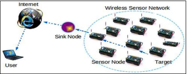
[image:18.595.160.481.601.728.2]A sensor network consists of a large number of sensor nodes that are deployed in a wide area with very low powered sensor nodes. The wireless sensor networks can be utilized as part of various information and telecommunications applications. The sensor nodes are very small devices with the capability of wireless communication, which collects information about sound, light, motion, temperature humanity and processed them before transferring it to the other nodes.
7 2.1.2 Characteristics of Sensor Nodes
Wireless Sensor Networks are:
(i). Self-configuration, Self-healing, Self -optimizing, and Self-protection. (ii). Capable of Short-range broadcasting communication and multi-hop
routing.
(iii). Dense deployment and cooperative effort of sensor nodes. (iv). Frequently changing topology due to fading and node failures.
(v). Severe limitations in energy capacity, computing power, memory, and transmitting power.
2.1.3 Sensor node architecture
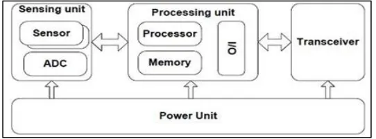
[image:19.595.185.456.395.495.2]A wireless sensor node is composed of four basic components, namely sensing unit, processing unit (microcontroller), transceiver unit and power unit.
Figure 2.2: Architecture of a typical sensor node
Figure 2.2 shows the typical construction of a sensor node. In addition to the above units, a wireless sensor node may include a number of application-specific components, for example, a location detection system or mobilizer. For this reason, many commercial sensor node products include expansion slots and support serial wired communication. Descriptions of the basic components are given below:
8 environment to sense data, e.g. radar) and may be directional or omnidirectional. A wireless sensor node may include multiple sensors providing complementary data. The sensing of a physical quantity such as those described, typically resulted in the production of a continuous analogue signal. For this reason, the sending unit is typically composed of a number of sensors and an analogue to digital converter (ADC) which digitizes the signal.
• Microcontroller: A microcontroller provides the processing power for, and coordinates the activity of, a wireless sensor node. Unlike the processing units associated with larger computers, a microcontroller integrates processing with some memory provision and I/O peripherals. Such integration reduces the need for additional hardware, wiring, energy and circuit board space. In addition to the memory provided by the microcontroller, it is not uncommon for a sensor node to include some external memory, for example, in the form of flash memory.
• Transceiver: A transceiver unit allows the transmission and reception of data to other devices connecting a wireless sensor node to a network. Wireless sensor nodes typically communicate using an RF (radio frequency) transceiver and a wireless personal area network technology such as Blue-tooth or the 802.15.4 compliant protocols ZigBee and MiWi. The 802.15.4 standard specifies the physical layer and mediumaccess control for low-rate, low-cost wireless communications, whilst proto-cols such as ZigBee and MiWi build upon this by developing the upper layers of the OSI Reference Model. The Bluetooth specification crosses all layers of the OSI Reference Model and is also designed for low-rate, low-cost wireless networking.
9 Wireless sensor networking has such sensor nodes, which are especially designed in such a typical way that they have a microcontroller which controls the monitoring, a radio transceiver for generating radio waves, and different types of wireless communicating devices and also ready with an energy source like a battery. The entire network worked simultaneously by using different dimensions of sensors and worked on the phenomenon of multi routing algorithm which is also termed as wireless ad hoc networking.
2.1.4 Types of Wireless Sensor Networks
Wireless sensor networks are deployed on land, underground, and underwater. A sensor network faces different challenges and constraints according to the environment in the sensor network deployed. There are five types of the wireless sensor network as discussed in (Yick, Mukherjee and Ghosal, 2008).
(i). Terrestrial Wireless sensor network. (ii). Underground Wireless sensor network. (iii). Underwater Wireless sensor network. (iv). Multimedia Wireless sensor network.
(v). Mobile Wireless sensor network.
2.1.5 Wireless Sensor Network Applications
Wireless sensor network has a lot of applications like security, monitoring, biomedical research, tracking, etc. Basically, these applications are very useful for emergency services. Sensor network is categorized into various classes such as Environmental data collection, military applications, security monitoring, sensor node tracking, health application, home application, and hybrid networks.
2.2 WSNs Challenges and Constraints
10 Data processing; (v) Scalability; (vi) Reliability; (vii) Responsiveness; (viii) Mobility; (ix) Power Efficiency; (x) Managing the design tradeoffs.
2.2.1 Limited energy
Reducing node energy consumption is vital in WSNs. In fact, because of the reduced size of the sensor nodes, the battery has low capacity, and the available energy is very limited. Despite this scarcity of energy, the network is expected to operate for a relatively long time. Given that replacing batteries are usually impossible, one of the primary design goals is to use this limited amount of energy as efficiently as possible.
2.2.2 Low-quality communications
Wireless communications are always less reliable and have less quality compared to wired communication. Besides, sensor networks are often deployed in harsh environments, and sometimes they operate under extreme weather conditions. In these situations, the quality of the radio communication might be extremely poor, and performing the requested collective sensing task might become very difficult.
2.2.3 Resource- constrained computation.
The resources are scarce in WSNs. Protocols for sensor networks must strive to provide the desired quality of service (QOS) in spite of the few available resources. 2.2.4 Data processing
11 2.2.5 Scalability
Scalability refers to the ability of the network to grow, in terms of the number of nodes, without excessive overhead. This is an important real world requirement, where networks must support more than the small handful of nodes typically in a pilot implementation. This is due to the network overhead that comes with the increased size of the network. In ad hoc networks, the network is formed without any predetermined topology or shape. Therefore, any node wishing to communicate with other nodes should generate more packets than its data packets, i.e., control packets or network overhead. As the size of the network grows, more control packets will be needed to find and keep the routing paths. Moreover, as the network size increases, there is a higher chance that communication links become broken in communication paths, which will end up creating more control packets. In a small network, the amount of control packets is almost negligible. However, when the network size starts increasing, the overhead increases rapidly. Since the available overall bandwidth is limited, the increase of overhead results in the decrease of usable bandwidth for data transmission. As the network size grows further, there is a very small amount of bandwidth left for application data transmission.
2.2.6 Reliability
12 and reliability are closely coupled, and typically, they act against each other.
2.2.7 Responsiveness
Responsiveness is the ability of the network to quickly adapt itself to changes in topology. High responsiveness can achieve in an ad hoc network, where the system issues more control packets, which will naturally result in less scalability and less reliability.
2.2.8 Mobility
Mobility refers to the ability of the network to handle mobile nodes and changeable data paths. Generally, a wireless sensor network that includes a number of mobile nodes should have high responsiveness to deal with the mobility. Therefore, it is not easy to design a large scale and highly mobile wireless sensor network.
2.2.9 Power Efficiency
Power efficiency, the ability of the network to operate at extremely low power levels, also plays an important role. A typical method for designing a low-power wireless sensor network is to reduce the duty cycle of each node. The drawback is that as the wireless sensor node stays longer in sleep mode to save power, there is less chance that the node can communicate with its neighbor’s. This decreases the network responsiveness, and also lowers reliably due to the lack of the exchange of control packets and delays in packet delivery. In addition, a more complicated synchronization technique will be necessary to keep more nodes in low duty cycle, which may also affect scalability.
2.2.10 Managing The Design Tradeoffs
13 in the design of wireless sensor networks, and there are always design tradeoffs. When choosing a wireless sensor network for an application, careful consideration of the balance of these factors within the context of the needs of the application is critical.
2.3 Wireless Sensor Networks Logical Topologies
In Wireless Sensor Networks (WSNs), topology plays an essential part in minimizing different imperatives, for example, latency, restricted vitality, computational asset emergency and nature of the correspondence.
2.3.1 Flat Logical Topology
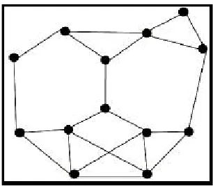
This is actually no topology, or the absence of any defined topology. In flat topology, each sensor plays an equal role in network formation. Different protocols have been proposed based on flat/unstructured topology (Mamun, 2012). For example, this flat topology has been used in data aggregation protocols (Xu and Wang, 2011), data gathering protocols (Fan and Sinha, 2007), node scheduling protocols (Sausen and Perkusichy, 2008), and routing protocols (Hussain and Islam, 2007). Figure 2.3
shows the flat topology architecture where the nodes are the sensors and the edges are available communication links between two sensors.
14
Figure 2.3: Flat logical topology (Mamun, 2012)
In a flat network, data aggregation is accomplished by data-centric routing where the BS usually transmits a query message to the sensor nodes via flooding, and the sensor nodes that have data matching in the query, will send response messages back to the BS. The sensor nodes communicate with the BS via multi-hop routes by using peer nodes as relays. The choice of particular communication protocol depends on a specific application.
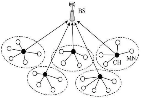
2.3.2 Cluster Logical Topology
[image:26.595.194.448.575.725.2]In general, when working with clusters it is possible to identify three main elements in the WSN: sensor nodes (SNs), base station (BS) and cluster heads (CH) (see Figure 2.4). The SNs are the set of sensors present in the network, arranged to sense the environment and collect the data. The main task of a SN in a sensor field is to detect events, perform quick local data processing, and then transmit the data. The BS is the data processing point for the data received from the sensor nodes, and where the data is accessed by the end-user.
15 It is generally considered fixed and at a far distance from the sensor nodes. The CH acts as a gateway between the SNs and the BS. The function of the cluster head is to perform common functions for all the nodes in the cluster, like aggregating the data before sending it to the BS. In some way, the CH is the sink for the cluster nodes, and the BS is the sink for the cluster heads. This structure is formed among the sensor nodes, the sink and the BS and is replicated as many times as it is needed, creating the different layers of the hierarchical WSN. The greatest constraint, it has is the power consumption, which usually is caused when the sensor is observing its surroundings, and communicating (sending and receiving) data.
2.3.2.1 Cluster Types
Clustering algorithms can be classified as Distributed Clustering and Centralized Clustering. Distributed clustering techniques are further classified into four sub types based on the cluster formation criteria and parameters used for CH election as based on identity, neighbourhood information, Probabilistic, and Iterative respectively (Geetha and Tellajeera, 2012).
2.3.3 Chain Logical Topology
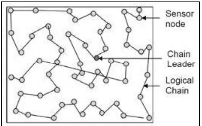
[image:27.595.218.421.593.720.2]Chain oriented topologies have been used by researchers in designing various protocols, among which data broadcasting protocols, data collection/gathering protocols and routing protocols are the major instances. Chain topologies are mainly used in these protocols to reduce the total energy consumption, and thus to increase the lifetime of the network.
16
2.4 Protocols of WSNs
When designing network protocols for wireless sensor networks, several factors should be considered. First and foremost, because of the scarce energy resources, routing decisions should be guided by some awareness of the energy resources in the network. Furthermore, sensor networks are unique from general ad hoc networks in that communication channel often exist between events and sinks, rather than between individual source nodes and sinks.
2.4.1 Low-Energy Adaptive Clustering Hierarchy (LEACH) Protocol
LEACH is a type of cluster-based routing protocols, which utilizes a distributed cluster formation. LEACH arbitrarily chooses a couple of sensor nodes as cluster heads (CHs) and turns this part to equitably circulate the energy load among the sensors in the system. The idea is to structure. And cluster the sensor nodes focused around those nodes that have signal quality and use neighborhood group heads as switches to the sink (Sharma and Verma, 2013). In LEACH, the Cluster Heads clamp information received all members of the cluster and send the collected packet to the base station keeping in mind the end goal to lessen the amount of data that must be transmitted to the BS. With a specific goal to diminish inter and intra - cluster obstruction LEACH utilizes a TDMA/code-division to ensure successful access (CDMA) to MAC. The operation of LEACH is carried out in two steps. The setup stage and the steady state. In setup stage the nodes are composed into clusters and CHs are chosen. These cluster heads change haphazardly about whether to keep in mind the goal to adjust the vitality of the system. This is carried out by picking an irregular number somewhere around 0 and 1 (Thakkar and Kotecha, 2014). The node is chosen as a CH for the present round if the random number is short of what the threshold value T (n), which is given by
( ) { ( )
( )
where
17 - is the Current round number and
- is the Group of nodes that have not been cluster head in the last 1/p rounds.
Here G is the number of nodes that are included in the previous round of CH elections. LEACH clustering is shown in Figure 2.6. In the steady state stage, the genuine information is exchanged to the base station. In order to minimize overhead the time of the steady state stage ought to be longer than the length of time on the setup stage. The CH node, in the wake of accepting all the information from its path nodes, has performed data collection before sending it to the base station. After a certain time period, the setup stage is restarted and new CHs are chosen. Each cluster communicates utilizing different CDMA codes to lessen impedance from nodes fitting in with different clusters. The strategies to accomplish the objectives of these are as follows:
Randomized, versatile, outlining toward oneself group development. Localized control of information exchanges.
Low vitality media access control (MAC).
[image:29.595.201.439.462.628.2] Application of particular information processing, for example, information accumulation and compression.
Figure 2.6: cluster head selection (Liu, 2012)
2.4.1.1 Operation of the LEACH
18 Cluster-head Advertisement.
Cluster Set-Up.
Transmission schedule creation.
And the stages of the steady state Phase (The cluster-head is maintained when data is transmitted between nodes):
Data transmission to cluster heads. Signal processing (Data fusion). Data transmission to the base station.
2.4.1.2 Cluster Head (CH) selection
For the selecting of the clusters-head nodes (Heinzelman, 2000)
( ) is the probability with which node i elects it to be (CH) at the beginning of the round r+1 (which starts at time t) such that the expected number of clusters-head nodes for this round is k.
[ ] ∑ ( ) ( )
where
N is the number of sensor nodes,
( ) is the is the probability with which node i elects it to be (CH), is the expected number of clusters-head.
Each node will be cluster head once in rounds.
Probability for each node i to be a cluster-head at time t, ( ) determines whether node i has been a cluster head in most recent (r mod(N/k)) rounds .
19
[∑ ( )
] ( ) ( )
∑ ( )
This ensures energy at each node to be approximately equal after every round. Using (2.3) and (2.4), the expected number of Cluster Heads per round is,
[ ] ∑ ( )
( ( ))
( )
2.4.1.3 Cluster Formation Algorithm
The cluster formation and the cluster head selection algorithm are given below: Step1: Initialization
Step2: if node i is CH processed from step3 to step7. If not returns to step1. Step3: CH broadcasts an advertisement message (ADV) using the CSMA
MAC protocol. ADV = node’s ID + distinguishable header.
Step4: Based on the received signal strength of ADV message, each non-Cluster Head node determines it’s non-Cluster Head for this round.
Step5: Each non-Cluster Head transmits a join-request message (Join-REQ) back to its chosen Cluster Head using a CSMA MAC protocol. Join-REQ = node’s ID + cluster-head ID + header.
Step6: Cluster Head node sets up a TDMA schedule for data transmission coordination within the cluster.
Step7: TDMA Schedule (1. Prevents collision among data messages. 2. Energy conservation in non-cluster-head nodes).
20
Figure 2.7: Distributed cluster formation algorithm (Heinzelman, 2000)
2.4.1.4 Sensor Data Aggregation
21 being observed. Therefore, mechanized routines for consolidating the data into a little set of compounded data are needed. In addition to helping avoid data over-burden, data aggregation, otherwise called data fusion, can consolidate a few untrustworthy data estimations to create a more accurate signal by improving the regular signal and lessening the uncorrelated noise. The manipulation performed on the collected data may be performed by a human administrator or off-hand (automatically). The method of performing data aggregation and the classification algorithm are application-specific. (Heinzelman, 2000).
In a routine sensor network, all the data are transmitted to the base station, where they are aggregated to obtain the data ( ). Automated strategies can then be used to characterize this aggregate signal (e.g., based on template source signatures). However, the function f can sometimes be broken up into several smaller functions
that operate on subsets of the data such that:
[image:33.595.159.478.407.535.2]( ) ( ( ) ( ) ( )) (2.5)
Figure 2.8: Block diagram of the Beamforming algorithm
22 [ ] ∑ ∑ [ ] [ ] (2.6) where
[ ] - is the signal from the sensor,
[ ] - is the weighting filter for the signal,
- is the total number of sensors, whose signals are being beamformed, - is the number of taps in the filter.
This algorithm is depicted in Figure 2.8. The weighting filters are chosen to satisfy optimization criteria, such as minimizing the mean squared error (MSE) or maximizing signal-to noise ratio (SNR). Various algorithms, such as least mean squared (LMS) error approach and the maximum power beamforming algorithm have been developed to determine good weighting filters. These algorithms have various energy and quality tradeoffs. For example, the maximum power beamforming algorithm is capable of performing blind beamforming, requiring no information about the sensor locations. However, this algorithm computation intensive, which will quickly drain the limited energy of the node. By determining the amount of computation needed to fuse the data from several sensor nodes and the associated energy and time costs to perform these signal processing operations, it is possible to determine the optimum tradeoff between computation and communication. For example, determine the optimal number of sensors to utilize in processing data to minimize the overall time until the solution is achieved given a simple line network. In general networks, there is no closed-form solution as there is in a linear network, but heuristics can be developed to achieve good tradeoffs between computation and communication.
23
The energy dissipation for local data aggregation and provender of sending the aggregate data can be analytically compared. Suppose that the energy dissipation per bit for data aggregation is and the energy dissipation per bit to transmit to the base station is . In addition, suppose that the data aggregation method can compress the data with a ratio of L:1. This means that for every L bits that must be sent to the base station when no data aggregation is performed, only 1 bit must be sent to the base station when local data aggregation is performed. Therefore, the energy to perform local data aggregation and transmit the aggregate signal for every L bits of data is:
( )
and the energy to transmit all L bits of data directly to the base station is:
( )
Therefore, performing local data aggregation requires less energy than sending all the unprocessed data to the base station when:
( )
where
- is the energy dissipation per bit for data aggregation,
- is the energy dissipation per bit to transmit to the base station, - is the data (bits) to transmit.
2.4.2 Power-efficient gathering in sensor information systems (PEGASIS) protocol
24 fact that the PEGASIS develops a tie associating all nodes to adjust system vitality scattering, there are still a few issues with this scheme.
For a substantial sensing field and ongoing applications, the single long chain may present an unsuitable information deferral time.
Since the chain pioneer is chosen by alternating, for a few cases, a few sensor nodes might reversely their amassed information to the assigned pioneer, which is far from the base station than itself. This will bring about excess transmission ways, and hence truly waste system energy.
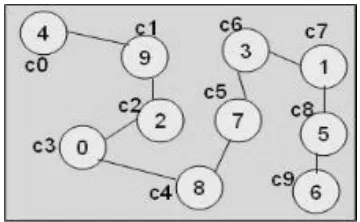
[image:36.595.234.414.288.399.2] The single chain leader may become a bottleneck.
Figure 2.9: Example for PEGASIS Chain
As shows in above Figure 2.9, amid each round, a pioneer node is arbitrarily chosen. The pioneer node is in charge of sending the accumulated information to the sink. Once the pioneer node is chosen and told by the sink node, every node on both sides of the bind (as for the pioneer node), goats and transmits the accumulated information to the following node in the chain, until the information achieves the pioneer node. For instance, consider the chain framed in Figure 2.9 for a 10-node system. The list of the nodes in the chain is different from the recognizable proof numbers for the nodes (i.e., the node ID). In the event that node 3 at chain record 6 is chosen as the pioneer node, the stream of information would be in the accompanying request: c0 -7 c1 -7 c2 -7 c3 -7 c4 -7 c5 -7 c6 PEGASIS can prompt critical defers in information collection in view of the holding up time at the pioneer node to get information from both sides of the chain.
2.4.2.1 Leader Selection
74
REFERENCES
Akyildiz, I.F., Su, W., Sankarasubramaniam, Y. & Cayirci, E. (2002). Wireless sensor networks: a survey. Computer networks, 38(4), pp. 393–422.
Ali, S.A. & Refaay, S.K. (2011). Chain-chain based routing protocol. International Journal of Computer Science Issues (IJCSI), 8(3).
Aliouat, Z., & Aliouat, M. (2012, March). Efficient management of energy budget for PEGASIS routing protocol. In Sciences of Electronics, Technologies of Information and Telecommunications (SETIT), 2012 6th International Conference on (pp. 516-521). IEEE.
Al-Karaki, J.N. & Kamal, A.E. (2004). Routing techniques in wireless sensor networks: a survey. Wireless communications, IEEE, 11(6), pp. 6–28.
Amis, A.D., Prakash, R., Vuong, T.H. & Huynh, D.T. (2000). Max-min d-cluster formation in wireless ad hoc networks. In: INFOCOM 2000. Nineteenth Annual Joint Conference of the IEEE Computer and Communications Societies. Proceedings. IEEE, volume 1, IEEE, pp. 32–41.
Chatterjee, M., Das, S.K. & Turgut, D. (2002). Wca: A weighted clustering algorithm for mobile ad hoc networks. Cluster Computing, 5(2), pp. 193–204. Chen, Y., Liestman, A.L. & Liu, J. (2006). A hierarchical energy-effcient framework for data aggregation in wireless sensor networks. Vehicular Technology, IEEE Transactions on, 55(3), pp. 789–796.
75
monitoring and measurement of heterogeneous wireless and wired networks, ACM, pp. 25–30.
Dave, P. M., & Dalal, P. D. (2013). Simulation & Performance Evaluation of Routing Protocols in Wireless Sensor Network. Simulation, 2(3).
Fan, K.W., Liu, S. & Sinha, P. (2007). Structure-free data aggregation in sensor networks. Mobile Computing, IEEE Transactions on, 6(8), pp. 929–942.
Furuta, T., Sasaki, M., Ishizaki, F., Suzuki, A. & Miyazawa, H. (2007). A New Clustering Algorithm Using Facility Location Theory for Wireless Sensor Networks. Technical report, Technical Report NANZAN-TR-2006-04, Nanzan Aca-demic Society.
Geetha, V., Kallapur, P. & Tellajeera, S. (2012). Clustering in wireless sensor networks: Performance comparison of leach & leach-c protocols using ns2. Procedia Technology, 4, pp. 163–170.
Ghaffarzadeh, H., & Doustmohammadi, A. (2014). Two-phase data traffic optimization of wireless sensor networks for prolonging network lifetime.Wireless networks, 20(4), 671-679
Gnanasekaran, T., & Francis, S. A. J. (2014, January). Comparative analysis on routing protocols in Wireless Sensor Networks. In Computer Communication and Informatics (ICCCI), 2014 International Conference on (pp. 1-6). IEEE.
Halgamuge, M., Zukerman, M., Ramamohanarao, K. and Vu, H. (2009). AN Estimation Of Sensor Energy Consumption. PIER B, 12, pp.259-295.
Haneef, M. (2012). Design Challenges and Comparative Analysis of Cluster Based Routing Protocols Used in Wireless Sensor Networks for Improving Network Life Time. Advances in Information Sciences & Service Sciences, 4(1). Hani, R. and Ijjeh, A. (2013). A Survey on LEACH-Based Energy Aware Protocols for Wireless Sensor Networks. JCM, 8(3), pp.192-206
76
Sciences, 2000. Proceedings of the 33rd Annual Hawaii International Conference on, IEEE, pp. 10–pp.
Heinzelman, W.R., Kulik, J. & Balakrishnan, H. (1999). Adaptive protocols for information dissemination in wireless sensor networks. In: Proceedings of the 5th annual ACM/IEEE international conference on Mobile computing and networking, ACM, pp. 174–185.
Heinzelman, W. B. (2000). Application-specific protocol architectures for wireless networks (Doctoral dissertation, Massachusetts Institute of Technology). Heinzelman, W. B., Chandrakasan, A. P., & Balakrishnan, H. (2002). An application-specific protocol architecture for wireless microsensor networks.Wireless Communications, IEEE Transactions on, 1(4), 660-670. Hussain, S. & Islam, O. (2007). An energy efficient spanning tree based multi-hop routing in wireless sensor networks. In: Wireless Communications and Networking Conference, 2007. WCNC 2007. IEEE, IEEE, pp. 4383–4388. Kumarawadu, P., Dechene, D.J., Luccini, M. & Sauer, A. (2008). Algorithms for node clustering in wireless sensor networks: A survey. In: Information and Automation for Sustainability, 2008. ICIAFS 2008. 4th International Conference on, IEEE, pp. 295–300.
Lindsey, S., Raghavendra, C. & Sivalingam, K.M. (2002). Data gathering algorithms in sensor networks using energy metrics. Parallel and Distributed Systems, IEEE Transactions on, 13(9), pp. 924–935.
Liu, X. (2012). A survey on clustering routing protocols in wireless sensor networks. Sensors, 12(8), pp. 11113–11153.
Loscri, V., Morabito, G. & Marano, S. (2005). A two-levels hierarchy for low-energy adaptive clustering hierarchy (tl-leach). In: IEEE Vehicular Technology Conference, volume 62, IEEE; 1999, p. 1809.
77
Mamun, Q. (2012). A qualitative comparison of different logical topologies for wireless sensor networks. Sensors, 12(11), 14887-14913.
Manjeshwar, A. & Agrawal, D.P. (2001). Teen: Arouting protocol for enhanced efficiency in wireless sensor networks. In: IPDPS, volume 1, p. 189.
Miller, M. J., & Vaidya, N. F. (2005). A MAC protocol to reduce sensor network energy consumption using a wakeup radio. Mobile Computing, IEEE Transactions on, 4(3), 228-242.
Sausen, P.S., Spohny, M. & Perkusichy, A. (2008). Energy effcient blind flooding in wireless sensors networks. In: Industrial Electronics, 2008. IECON 2008. 34th Annual Conference of IEEE, IEEE, pp. 1736–1741.
Sharma, N. & Verma, V. (2013). Energy efficient leach protocol for wireless sensor network. International Journal of Information and Network Security (IJINS), 2(4), pp. 333–338.
Thakkar, A., & Kotecha, K. (2014). Alive Nodes Based Improved Low Energy Adaptive Clustering Hierarchy for Wireless Sensor Network. In Advanced Computing, Networking and Informatics-Volume 2 (pp. 51-58). Springer International Publishing.
Wang, A. and Chandrakasan, A. (2002). Energy-efficient DSPs for wireless sensor networks. IEEE Signal Process. Mag., 19(4), pp.68-78.
Wang, J., Tang, B., Zhang, Z., Shen, J., & Kim, J. U. (2014). An Energy Efficient Data Dissemination Algorithm for Wireless Sensor Networks.PP.1-6.
Xu, X., Li, M., Mao, X., Tang, S. & Wang, S. (2011). A delay-effcient algorithm for data aggregation in multihop wireless sensor networks. Parallel and Distributed Systems, IEEE Transactions on, 22(1), pp. 163–175.
78
Yick, J., Mukherjee, B. & Ghosal, D. (2008). Wireless sensor network survey. Computer networks, 52(12), pp. 2292–2330.
Younis, O. & Fahmy, S. (2004). Heed: a hybrid, energy-effcient, distributed clustering approach for ad hoc sensor networks. Mobile Computing, IEEE Transactions on, 3(4), pp. 366–379.
Yu, L., Wang, N., Zhang, W. & Zheng, C. (2006). Group: A grid-clustering routing protocol for wireless sensor networks. In: Wireless Communications, Networking and Mobile Computing, 2006. WiCOM 2006. International Conference on, IEEE, pp. 1–5.
Yuan, L., Zhu, Y. & Xu, T. (2008). A multi-layered energy-effcient and delay reduced chain-based data gathering protocol for wireless sensor network. In: Mechtronic and Embedded Systems and Applications, 2008. MESA 2008. IEEE/ASME International Conference on, IEEE, pp. 13–18.