Munich Personal RePEc Archive
The long-term decline of internal
migration in Canada – Ontario as a case
study
Basher, Syed A. and Fachin, Stefano
Qatar Central Bank, University or Rome "La Sapienza"
January 2008
Online at
https://mpra.ub.uni-muenchen.de/6685/
The long-term decline of internal migration
in Canada – Ontario as a case study
∗
Syed A. Basher
†Qatar Central Bank
Stefano Fachin
‡University of Rome ‘La Sapienza’
January 9, 2008
Abstract
Migration between the Canadian provinces generally followed a declining trend over the period 1971-2004. In this paper, taking Ontario a case study, we seek to ex-plain these patterns using recent panel cointegration methods that are robust to cross-section dependence. Estimation of heterogenous models suggests that the de-terminants of migration vary across provinces. Overall, unemployment differential and income in the sending province appear to be the most important ones, with income and federal transfer differentials playing only a minor role.
Keywords: Internal migration; panel cointegration; bootstrap; Canada.
JEL Classification: C32; C33; R23.
1
Introduction
Canada has a long tradition of internal migration stretching from 1950s to the present day.
Research over the last four decades on the spatial pattern of migration in Canada brings
∗The views expressed here are those of author(s) and do not reflect the official view of the Qatar
Central Bank. Fachin gratefully acknowledges financial support from University of Rome ‘La Sapienza’ and MIUR.
†Department of Economic Policies, Qatar Central Bank, P.O. Box 1234, Doha, Qatar. E-mail:
‡Corresponding author: Facolt`a di Scienze Statistiche–DCNAPS, Box 83, RM 62, Universit`a di Roma
out the following stylized facts. Throughout this long period three economically strong
provinces–Ontario, British Columbia, and Alberta–have been the principal net gainers
from interprovincial migration; whereas the remaining seven economically weak provinces
tended to be the consistent net losers through internal migration. Stronger economic
growth and better employment opportunities are often taken to be the explanation of the
regional pattern of migration between the two sets of provinces.1
Persistent change in
internal population redistribution over the 1951-2001 period has helped Ontario, British
Columbia, and Alberta to increase their share of Canadian population by an average of
4.6%, while the average share for the remaining seven provinces decreased by nearly 3.3%
(Liaw and Xu, 2005). In the last three decades this trend somehow has slowed down, so
that the 1971-2004 averages are respectively 2.8% and -1.2% (see Table 1).
Since the impact of internal migration on the distribution of population across provinces
has been substantial2
it is not surprising that there is by now a fairly substantial literature
on interprovincial migration based on both micro and aggregate data.3
Although internal migration has been an integral part of Canada’s population
dynam-ics, interestingly very little has changed in terms of specific migration flows among the
provincial origins and destinations. More than 30 years later we see that the spatial
pat-tern of migration in Canada is very much in line with the observation first made by Stone
(1974). In other words, Ontario still is the most favorite destination for out-migrants
from Quebec and the four Atlantic4
provinces. On the other hand, out-migrants from the
western provinces (Alberta and British Columbia) mainly choose other western provinces
as their most favored destinations. Importantly, there are no large streams originating in
either British Columbia or Alberta and ending east of Ontario; whereas Ontario ranked
second as a destination for out-migrants from the two westerly provinces. In this respect,
Ontario is like a sort of “buffer zone” inhibiting strong flows between the eastern and
western regions of Canada (see Stone, 1969, 1974).
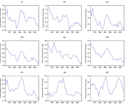
Nevertheless, an important observation that, to the best of our knowledge, has been
overlooked in the literature is the fact that gross migration flows from both eastern and
1
See, for instance, Table 1 in Liaw and Xu (2005).
2
The annual average (between 1971-2004) migration flow from one province to another is approxi-mately 31,279 persons, or 1.17% of the total population (excluding the territories).
3
For review of pre-1975 work see Stone (1974). Day and Winner (1994) extensively cover pre-1995 literature, while Finnie (2004) offers a long list of related work on internal migration.
4
western provinces to Ontario have been declining steadily over the years (see Figure
1). Save for British Columbia, the logarithm of gross migration flows to Ontario is
mostly trending downward, with only some temporary upward swings around the early
1990s. This is interesting, as Ontario has consistently been one of the most attractive
provinces in terms of both income and employment opportunities. What is the cause of
the declining trend in migration flows to Ontario from rest of Canada, particularly the
eastern provinces? Only the narrowing of income gap and unemployment differentials, or
have other factors been at play?
Our goal in this article is to empirically examine the long-run determinants of this
decline using a panel of interprovincial migration data from 1971-2004. Obviously, there
have been several attempts to explain interprovincial migration pattern using long-span
data. Courchene (1970) uses family allowance data over 1952-1967 and observes a positive
association between rates of migration flows and ratios of earned income per employed
person between Canadian provinces. Vanderkamp (1971) observes a stronger positive
association between in-migration and earnings than a negative association between
out-migration and earnings for Canadian interprovincial flows during the period 1947-1966.
Shaw (1986) finds that fiscal variables (e.g. unemployment insurance) matter more over
traditional market variables (e.g. job creation or wages) for Canadian migration during
the period of 1956-1981. Day and Winer (2006) use individual tax records to construct
in-migration and out-migration data over the period 1974-1996 and find that regional
differences in (fiscal) policy variables do not have significant influence on interprovincial
migration. Finally, both Day and Winer (2006) and Coulombe (2006) point the
impor-tance of structural factors such as regional differences in earnings, employment prospects,
and labor productivity as the main drivers of interprovincial migration in Canada.
However, all these empirical studies share a serious methodological weakness: the
problem of non-stationarity of the data is never taken into account. In fact, the issue
of non-stationarity seems to be largely ignored even in the most recent contributions to
the empirical literature on interprovincial migration in Canada (e.g. Day and Winer,
2006; and Coulombe, 2006). Therefore, the objective of this paper is to fill the gap
in the literature by applying recent advances in panel data econometrics to examine
the long-run determinants of interprovincial migrations in Canada over the period
framework can clearly be used to study the migration behavior in other provinces.
Our paper is closely related to the strand of literature that examines regional disparity
in income across Canadian provinces. As such, convergence in income is likely to reduce
the economic motivation for migration, while absence or lack of convergence, on the
opposite, is likely to trigger migration from poorer to the richer provinces. Using
cross-sectional methods Coulombe and Lee (1995) and Coulombe and Day (1999) show that
poor provinces tend to grow faster than rich ones in per capita terms during the period
1961-1991. Based on unweighted standard deviation of relative income across Canadian
provinces Helliwell (1996) concludes that there was no significant differences in the rate
of income convergence between 1926-1960 and 1960-1990. Afxentiou and Serletis (1998)
applying cointegration approach are unable to find any support for convergence from 1961
to 1991. By contrast, DeJuan and Tomljanovich (2005) find overwhelming evidence of
economic convergence for most part of Canada over the period 1926 to 1996. In particular,
they observe very strong convergence evidence particularly in the Atlantic and Plains5
provinces.
In light of these findings it seems that while complete convergence (equilibrium) for
all provinces may not been achieved, there seem to be a rather general consensus on the
existence of a process of convergence. The increased efforts by the federal government
to establish interprovincial redistribution programs (i.e. equalization payments) may
have facilitated such convergence process (e.g. Kaufman et al., 2003; Rodriguez, 2006).
Therefore, one could argue that a possible explanation for the steady decline in migration
flows into Ontario is the increasing disappearance of regional income disparity within
Canada. We agree to this view and incorporate these ideas in our analysis.
The rest of the paper is organized as follows. Section 2 describes data and empirical
model. Section 3 briefly reviews the econometric methodology used. Section 4 presents
the empirical results. Section 5 concludes. All additional materials are presented in the
Appendix.
5
2
Modeling Internal Migrations: Data and Models
The primary source of our data is Statistics Canada6
, which records annual migration
streams by province of origin and destination. The advantage of using migration data with
adefined origin anddefined destination is that it will allow us to see how the provinces of
origin react to economic fundamentals when choosing Ontario as their favorite destination.
In particular, we will be able to ascertain why one region respond to more of a certain
kind of attributes than another. The disadvantage is that the data do not come by age
or sex group which makes the approach aggregate in nature. However, given our goal to
understand the long-run determinants of the declining migration inflows to Ontario, the
benefits of using origin-destination migration stream outweigh the costs.
Let us now discuss the variables used in some detail. First of all, the dependent
variable. Since our focus is on the destination region, Ontario, we normalize the migration
flows with the population in this province. Letting the home areah and the destination
area i, mht = P op−1
t Mht, where Mht is the total migration flow from h to Ontario and P opt is the total population in Ontario, at time t.
The explanatory variables are those typically used in previous studies, such as
Courch-ene (1970), Shaw (1986), and Osberg et al. (1994). According to standard models the
key determinant of migrations is the expected income differential, which, assuming for
simplicity static expectations, is a function of current unemployment and income
differ-entials. To capture the growth in the ability to support the unemployed population we
include in the model log income per capita in the home region as well. In both cases
we use disposable income, thus taking into account the regional differences in income
tax rates. In addition, we have also included per capita federal transfer differentials
between origin and destination provinces. Federal transfers, which includes the
equaliza-tion payment7
and unemployment benefits, are an important determinant of the so-called
“fiscally-induced migration” (e.g. Day and Winer, 2006). Formally, the log differentials
between h and Ontario are defined as xd
hit = xht−xit, x = y, u, g, with the symbols y, u, and g indicating log of disposable income per capita, unemployment rate, and federal
transfer per capita, respectively, and i= Ontario.
Finally, we include a measure of migration chain effect. Migrants are known to move
6
A detailed data source list is provided in Appendix A.
7
with a higher probability to destinations where people from the same area have moved to
in the past, as it is easier both to obtain information and to receive material support when
settling down.8
Considering that the probability of accessing information and support
is proportional to that of a contact with a past migrant, we define as a measure of the
migration chain effect the total migrations from the home area to the destination area
over the previous three years9
, divided by the total population of the home area: more
precisely, cht=P op−1 ht
P3
s=1Mh,t−s.
The starting model for our empirical analysis is then the following:
mhit =β0h+β1hydhit+β2hiudhit+β3higdhit+β4hyht+β5hchit+εht (1)
where h = home = NL, PE,...,BC, i= destination = ON, with h6=i;t = 1974, ...,2004,
as some initial observations are needed to initialize the migration chain variable.
Anticipating the sign of slope parameters, an increase in yd, gd, and y in the home
area is likely to reduce the (out) migration flows to Ontario. Therefore, we expect the
slope parameters to obey β1 <0, β3 <0, and β4 < 0. While, it is expected thatβ2 >0
andβ5 >0 as higher unemployment differentials and higher values of the migration chain
variable are expected to foster migration.
3
Econometric Methods
Since we are interested in the long-run patterns we need to carry out cointegration
analy-sis, first testing if (1) describes an equilibrium relationship, and, provided this is the case,
estimating the values of the coefficients. However, with only 31 time periods, the power
of conventional cointegration tests is known to be very low. Fortunately, a solution is
readily available: considering each origin-destination pair as a “unit” our dataset is
nat-urally seen as a panel, with the number of units N = 9 and that of time observations
T = 31. We can thus obtain higher power by applying some panel cointegration tests.
By now there exists a burgeoning literature on non-stationary panels suggesting
nu-8
An obvious example is the frequent case of male heads of families migrating alone first, with their wives and children joining them after some time.
9
merous panel estimators and tests for panel cointegration.10
. The advantage of using
panel data approach over standard time series methods is that by combining the
infor-mation coming from both the cross-section and the time dimensions, the power of the
tests can be increased, even without imposing any homogeneity assumption. When
deal-ing with panel data, it is important to keep in mind the issue of cross-section dependence
due to common trends and cycles in output across Canadian provinces (e.g., Wakerly et
al., 2006). Ignoring the cross-section correlation is known to cause severe size distortion
(e.g. Banerjee et al., 2004), so that the power gain delivered by the panel dimension,
which is the very reason for its use, is entirely fictitious.
In this paper, we apply the bootstrap panel cointegration tests recently proposed
by Fachin (2007). This test is robust to both short- and long-run dependence across
units and delivers good small sample performances, which is important since in our case
N = 9. The basic principle of this test11
is to compute a summary statistic (say, G) of
the no cointegration tests for the individual units on the empirical data set and on a large
number of pseudo-datasets constructed under the null hypothesis of no cointegration (say,
G∗). The no cointegration hypothesis is rejected if the empirical statistic G falls in the
tail of the distribution of the G∗′s; in the classical Engle-Granger cointegration test, if
the bootstrapp-value p∗ =prop(G∗ <Gb) is small. Clearly, a key point of the procedure
is the construction of the series under no cointegration. These are obtained applying
Paparoditis and Politis (2001) Continuous-Path Block Bootstrap (CBB); more details,
which are beyond the scope of this paper, are given in Fachin (2007). Natural choices
of summary statistics are the mean (G = N−1PN
i=1ADFi, where ADFi is the ADF
statistic computed on the residuals of thei−th cointegrating regression) corresponding
to Pedroni (1999) Groupt-statistic, and the median,Gme =M edian(ADF
1, . . . , ADFn).
In both cases the null hypothesis is ‘cointegration in no units’, against the alternative
hypothesis ‘cointegration in a large number of units’. Hence, in case of rejection we are
not implying that in the specific time sample at hand cointegration holds in all units.
Rather, we are implicitly taking what we may define a democratic stance: since the
units are reasonably homogenous, if a long-run equilibrium exists in most of them, the
exceptions are regarded as due to temporary conditions, which will vanish asymptotically.
As mentioned above, if cointegration is found to hold we can proceed to estimate the
10
See Breitung and Pesaran (2007) and the references therein for an overview of the field.
11
coefficients of the long-run relationships. From model (1) letting h = N L, . . . , BC, we
obtain a system of nine equations. This system is likely to be characterised by strong
correlation of the disturbances and cointegration of the explanatory variables across
equa-tions. The first point would suggest that efficiency gains may be obtained applying SUR
estimation methods (such as FM-SUR by Moon, 1999, or DGLS by Mark, Ogaki and Sul,
2005). Unfortunately, all these methods require the inversion of the long-run covariance
matrix of the system, singular under cointegration across units, and are thus not feasible.
Howewer, the issue is not as serious as it might appear: according to simulation results by
Moon and Perron (2005), the efficiency gains delivered by SUR estimators with respect
to single-equation estimators such as FM-OLS are in fact essentially negligible. We can
thus safely proceed to separate estimation by FM-OLS of each individual equation.
3.1
Testing for Cross-section Dependence in Panels
Recent developments in the literature offer the possibility of testing for the presence of
cross-section dependence among individuals. Pesaran (2004) presents a simple test of
error cross-section dependence that is valid asymptotically under very general conditions
and can be applied to both stationary and non-stationary panels. The test statistic
based on the average of pair-wise Pearson’s correlation coefficients ˆpj, j = 1,2, . . . , n,
n = N(N−1)/2, of the residuals obtained from the estimation of autoregressive (AR)
regression models. The CD statistic in Pesaran (2004) is given by
CD =
r
2T n
n X
j=1
ˆ
pj →N(0,1) (2)
This statistic tests the null hypothesis of cross-section independence against the
alter-native hypothesis of dependence. Simulation results in Pesaran (2004) show that the
statistic has reasonably good finite sample performance in terms of size and power.
4
Empirical Results
We first examined the time series properties of the series with individual ADF unit root
tests, reported in Table 2. Consistently with our expectations, the migration rates are
cases the deterministic kernel has been chosen on a priori grounds, with a linear trend
respectively included in the latter and excluded in the former. In the the remaining
cases (income, unemployment and federal transfer differentials) we followed the selection
procedure proposed by Ayat and Burridge (2000), including a deterministic trend when
significant.12
As to be expected, this criterion leads always to tests with constant only in the case
of the unemployment differential, while for the other two differentials both cases are
present. For the income differential the I(1) hypothesis is never rejected except one case,
at the 5%, while this happens in three cases for the unemployment differential. For both
variables there are no rejections at 1%. The federal transfer differentials appear somehow
more stationary, with three rejections at 5% and two at 1% (Quebec and Newfoundland
and Labrador). We decided to take a rather conservative stance, excluding from the
initial models only the variables found stationary at 1%. Also, given the results on the
migration rates we always included a migration chain variable.
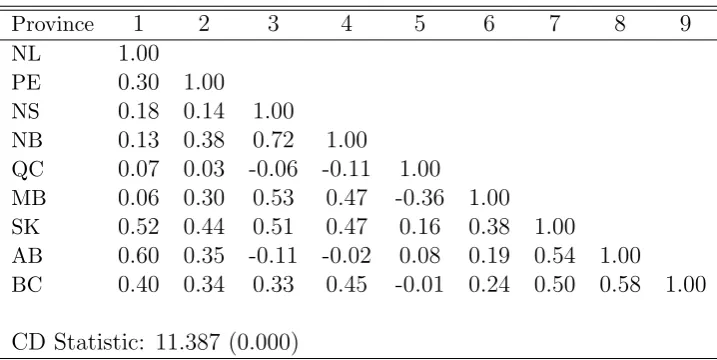
To get a feeling of the size of the cross-section dependence problem in the data, we
have computed some cross-correlation tests. The results are summarized in Table 3.
The short-run cross-section correlations are based on the regression residuals obtained
from (1). At first sight, there seem to be only moderate evidence of cross-correlation in
the data, as only 16 out of 36 cross-correlations are significant according to the usual
approximate critical bounds. However, the average absolute correlation13
between all the
cross-section units is 0.382, which is not negligible. Further, Pesaran’s (2004) CD statistic
strongly rejects the null hypothesis of no cross-section dependence at least at the 1% level
of significance. Hence, overall there seems to be enough evidence suggesting the presence
of cross-section dependence in model (1), confirming the need to apply a robust testing
procedure.
The results of panel cointegration tests with fully heterogenous specification (fixed
effects, heterogenous slopes) are reported in the top panel of Table 4, and FM-OLS
estimates of the individual equations in the bottom part of the same table. The bootstrap
12
Although the idea of a linear trend in a differential may appear not plausible, this is not actually the case. If the linear trend enters the univariate Data Generating Processes of a variable with differ-ent coefficidiffer-ents in the home and destination regions the differdiffer-ential will have a linear trend also, with coefficient the difference of the regional coefficients.
13
algorithm used 1000 redrawings and block length fixed at 4. The p-values for both the
mean and median of the individual ADF statistics are all very small14
, indicating that
that the models specified are cointegrating relationships. We can then examine the
FM-OLS estimates of the cointegrating coefficients. For brevity, we report only the final
specifications15
.
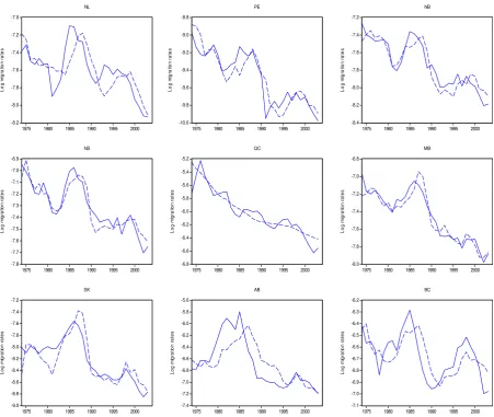
The plots of the series and FM-OLS estimates, shown in Figure 2, reveal that the
models manage to capture rather accurately both the main trends and some local swings.
The income differential (yd) enters only in the equations for three Atlantic provinces (NL,
PE, NB) but with a very large elasticity. Compared to this, home income (y) might seem
to be a more important explanatory variable, as it enters in five equations. However, its
elasticity is always rather small (average around 0.46 in absolute value).
Save for Alberta, we see that migrations originating in the westerly provinces are more
likely to respond to changes in home income, while the case is quite mixed for provinces
located east of Ontario with three out five home areas responding strongly to income
differential. As argued in Faini et al. (1997), a higher home income implies that it may
have become easier for households to finance protracted period of unemployment of some
of their members causing migration flow to decrease.16
The unemployment differential (ud) enters in seven equations with a near average of
unit elasticity. As can be seen, migrations originating in the western provinces respond
comparatively more strongly than those of the eastern provinces, in particular the Atlantic
ones. This is not surprising given the more generous unemployment benefits existing in
the maritime provinces compared to other provinces17
. It is instead somehow puzzling to
find that Manitoba and Saskatchewan react strongly to the unemployment differential,
since their condition compared to the average of the provinces has improved or remained
approximately constant (see Table 1).
14
Note that the FDB p-values, computed through Davidson and MacKinnon’s (2000) Fast Double Bootstrap, are very close to the base boostrap values, suggesting these to be very reliable.
15
Given the small time sample available we followed the model selection procedure discussed in Fachin (2007).
16
We are assuming that income was always high enough to make the financing effect (higher home income making it easier to finance the costs of migration, resulting a positive income-migration link) irrelevant.
17
Next, federal transfer differential (gd) is seen to be relevant for the two most western
provinces, while the migration chain (c) measure is relevant only for the three Atlantic
provinces. The latter indicates that family and friends who have previously migrated
from the Atlantic region to Ontario may have provided important information about
their present location which may have made the social transition easier for new migrants
from their former locality.
Summing up, our estimates, in line with previous work on interprovincial migration
in Canada (e.g. Helliwell, 1996; Day and Winer, 2006; and Coulombe, 2006), suggest the
existence of a very strong link between unemployment and migrations. The evidence on
income effect is mixed, with the level of home income appearing more important than
relative income differentials.
5
Conclusions
We started our study from the observation that migration from the Canadian provinces
towards Ontario mostly followed a declining trend over the period 1971-2004. In view of
the process of convergence in both income and labour market conditions which, though
by no means complete, did however took place during this period this is not surpring.
However, important questions are open: is the convergence process really the
explana-tion for these migraexplana-tion trends? Have income and labour market condiexplana-tions been equally
important? Given the small time sample studying this phenomenon using conventional
cointegration methods would be difficult; further, strong short- and long-run cross-section
dependence make the most popular asymptotic panel cointegration tests unfit. The
so-lution is provided by the bootstrap panel cointegration test recently proposed by Fachin
(2007). Applying this test we have been able to reach rather clear conclusions. First
of all, a rather small and natural set of determinants (income, labor market and fiscal
differentials, income in the sending provinces) is able to explain the observed declining
trends. Second, estimation of heterogenous models suggests that the determinants of
mi-gration vary across provinces, with unemployment differential and income in the sending
province the most important explanatory ones. Income and federal transfer differentials
appear to play only a minor role.
significantly reduced by shrinking differentials in the labour market and income growth
in the sending provinces. At this point, an obvious remark is that our macro approach
leaves open a natural and important question: if unemployment in a province tends to
increase the outmigration of labor force from that province, who is more likely to move?
The unemployed, or, rather, those already employed? Unfortunately data limitation does
not permit us to shed light on this important question. Lack of data also prevent us to
analyze movements in intraprovincial migration which plays even more important role
in labour market adjustment than interprovincial migration (e.g. Lin, 1995). With the
6
Appendix A. Data
All data are annual and come from Statistics Canada’s E-STAT database. All income figures are expressed in Canadian dollar, while per capita figures are obtained by nor-malising by the population. The data is available from the corresponding author on request.
• Migration (persons): Interprovincial migration flow data by province of origin and destination, 1971/72 to 2005/06, E-STAT Table 051-0019. For convenience, we treat annual years as 1971 to 2004.
• Population (persons): Total population by province, 1971 to 2006, E-STAT Table 051-0001.
• Disposable income (dollar): Personal disposable income by provinces, 1981 to 2004, E-STAT Table 384-0013. Data for the period 1971-1980 is available from E-STAT Table 384-0035.
• Unemployment rate (percent): Data for 1976-2004 is taken from E-STAT Table 282-0002. Remaining data for 1971-1975 come from E-STAT Table 384-0035.
• Federal transfer (dollar): Federal government current transfer to persons, 1981-2004, E-STAT Table 384-0004. Remaining data for 1971-1980 come from E-STAT Table 384-0022.
7
Appendix B. Bootstrap algorithm
Denoting by G a summary statistic of the no cointegration tests for the individual units (e.g. G=N−1PN
i=1ADFi, orG=M edian(ADF1, . . . , ADFn),whereADFi is theADF
statistic computed on the residuals of the i−th cointegrating regression) the proposed bootstrap procedure includes five simple steps:
1. compute the Group statistic Gb for the data set under study,
{X1X2. . . XN, Y1Y2. . . YN}Tt=1;
2. construct separately by CBB two sets of N pseudo-series,
{X∗
1X2∗. . . XN∗} T∗
t=1 and {Y1∗Y2∗. . . YN∗} T∗
t=1;
3. compute the Group statistics G∗ for the pseudo-data set,
{X∗
1X2∗. . . XN∗, Y1∗Y2∗. . . YN∗} T∗
t=1;
4. repeat steps (2) and (3) a large number (say, B) of times;
References
Afxentiou, P.C. and Serletis, A. (1998). Convergence across Canadian provinces. Cana-dian Journal of Regional Science 21, 11-26.
Ayat, L. and Burridge, P. (2000). Unit root tests in the presence of uncertainty about the non-stochastic trend. Journal of Econometrics 95, 71-96.
Banerjee A., Marcellino, M. and Osbat C. (2004). Some cautions on the use of panel methods for integrated series of macro-economic data. Econometrics Journal 7, 322-340.
Breitung, J. and Pesaran, M.H. (2007). Unit roots and cointegration in panels; forth-coming in L. Matyas, and P. Sevestre, The Econometrics of Panel Data (Third Edition), Kluwer Academic Publishers.
Coulombe, S. and Lee, F.C. (1995). Convergence across Canadian provinces, 1961 to 1991. Canadian Journal of Economics 28, 886-898.
Coulombe, S. and Day, K.M. (1999). Economic growth and regional income disparities in Canada and the northern united states. Canadian Public Policy 25, 155-178.
Coulombe, S. (2006). Internal migration, asymmetric shocks, and interprovincial eco-nomic adjustments in Canada. International Regional Science Review 29, 199-223.
Courchene, T.J. (1970). Interprovincial migration and economic adjustment. Canadian Journal of Economics 3, 550-76.
Davidson R. and MacKinnon, J.G. (2000). Improving the reliability of bootstrap tests. Queen?s University Institute for Economic Research Discussion Paper No. 995.
Day, K.M. and Winer, S.L. (1994). Internal migration and public policy: An introduc-tion to the issues and a review of empirical research in Canada; in A. Maslove (ed.), Issues in the Taxation of Individuals. Toronto: University of Toronto Press.
Day, K.M. and Winer, S.L. (2006). Policy-induced internal migration: An empirical investigation of the Canadian case. International Tax and Public Finance 13, 535-564.
DeJuan, J. and Tomljanovich, M. (2005). Income convergence across Canadian provinces in the 20th century: Almost but not quite there. Annals of Regional Science 39, 567-592.
Fachin, S. (2007). Long-run trends in internal migrations in Italy: A study in panel cointegration with dependent units. Journal of Applied Econometrics 22, 401-428.
Faini R., Galli G., Gennari P. and Rossi F. (1997). An empirical puzzle: Falling mi-gration and growing unemployment differentials among Italian regions. European Economic Review 41, 571-579.
Helliwell, J.F. (1996). Convergence and migration among provinces. Canadian Journal of Economics 29, Special Issue: Part 1, 324-330.
Kaufman, M., Swagel, P. and Dunaway, S. (2003). Regional convergence and the role of federal transfers in Canada. IMF Working Papers 03/97, International Monetary Fund.
Liaw, K-L. and Xu, L. (2005). Problematic post-landing migration of the immigrants in Canada: From 1980-82 through 1992-95. Journal of Population Studies 31, 105-152.
Lin, Z. (1995). Interprovincial labour mobility in Canada: The role of unemployment insurance and social assistance. Ottawa: Human Resources Development Canada.
Mark, N.C., Ogaki, M. and Sul, D. (2005). Dynamic seemingly unrelated cointegrating regressions. Review of Economic Studies 72, 797-820.
Moon, H.R. (1999). A note on fully-modified estimation of seemingly unrelated regres-sions models with integrated regressors. Economics Letters 65, 25-31.
Moon, H.R. and Perron, B. (2004). Efficient estimation of the SUR cointegration model and testing for purchasing power parity. Econometric Reviews 23, 293-323.
Osberg, L., Gordon, D. and Lin, Z. (1994). Interregional migration and interindus-try labour mobility in Canada: A simultaneous approach. Canadian Journal of Economics 27, 58-80.
Paparoditis E. and Politis, D.N. (2001). The continuous-path block bootstrap. In Asymptotics in Statistics and Probability: Papers in honor of George Roussas, Madan P (ed.). VSP: Zeist, Netherlands; 305-320.
Pedroni, P. (1999). Critical values for cointegration tests in heterogeneous panels with multiple regressors. Oxford Bulletin of Economics and Statistics 61, 653-670.
Pesaran, M.H. (2004). General diagnostic tests for cross section dependence in pan-els. Cambridge Working Papers in Economics No. 0435, Faculty of Economics, University of Cambridge.
Rodr´ıguez, G. (2006). The role of the interprovincial transfers in the : Further empirical evidence for Canada . Journal of Economic Studies 33, 12-29.
Shaw, R.P. (1986). Fiscal versus traditional market variables in Canadian migration. Journal of Political Economy 94, 648-666.
Stone, L.O. (1969). Migration in Canada: Some regional aspects. Ottawa: Dominion Bureau of Statistics.
Stone, L.O. (1974). What we know about migration within Canada – A selective review and agenda for future research. International Migration Review 8, 267-281.
Vanderkamp, J. (1971). Migration flows, their determinants and the effects of return migration. Journal of Political Economy 79, 1012-31.
8.0 8.2 8.4 8.6 8.8 9.0 9.2
1975 1980 1985 1990 1995 2000
NL 6.2 6.4 6.6 6.8 7.0 7.2 7.4
1975 1980 1985 1990 1995 2000
PE 8.6 8.8 9.0 9.2 9.4
1975 1980 1985 1990 1995 2000
NS 8.0 8.2 8.4 8.6 8.8 9.0 9.2
1975 1980 1985 1990 1995 2000
NB 9.6 9.8 10.0 10.2 10.4 10.6 10.8
1975 1980 1985 1990 1995 2000
QC 8.2 8.4 8.6 8.8 9.0 9.2 9.4
1975 1980 1985 1990 1995 2000
MB 7.4 7.6 7.8 8.0 8.2 8.4 8.6
1975 1980 1985 1990 1995 2000
SK 8.8 9.2 9.6 10.0 10.4
1975 1980 1985 1990 1995 2000
AB 9.0 9.2 9.4 9.6 9.8
1975 1980 1985 1990 1995 2000
[image:17.595.76.514.97.463.2]BC G ros s m igr at ion f low s (l ogs ) G ros s m igr at ion fl o w s ( logs ) G ros s m igr at io n f low s ( logs ) G ro s s m igr at io n f lo w s ( logs ) G ros s m ig rat ion f low s ( logs ) G ros s m igr at ion fl ow s ( lo gs ) G ros s m igr at ion f low s ( logs ) G ros s m igr at ion f low s ( logs ) G ros s m igr at ion f low s ( logs )
-8.2 -8.0 -7.8 -7.6 -7.4 -7.2 -7.0
1975 1980 1985 1990 1995 2000
L og m igr at ion r at e s NL -10.0 -9.8 -9.6 -9.4 -9.2 -9.0 -8.8
1975 1980 1985 1990 1995 2000
L og m igr at ion r at e s PE -8.4 -8.2 -8.0 -7.8 -7.6 -7.4 -7.2
1975 1980 1985 1990 1995 2000
L og m igr at ion r at e s NB -7.8 -7.7 -7.6 -7.5 -7.4 -7.3 -7.2 -7.1 -7.0 -6.9
1975 1980 1985 1990 1995 2000
Lo g m igr a tio n ra tes NS -6.8 -6.6 -6.4 -6.2 -6.0 -5.8 -5.6 -5.4 -5.2
1975 1980 1985 1990 1995 2000
Lo g m igr a tio n ra tes QC -8.0 -7.8 -7.6 -7.4 -7.2 -7.0 -6.8
1975 1980 1985 1990 1995 2000
Lo g m igr a tio n ra tes MB -9.0 -8.8 -8.6 -8.4 -8.2 -8.0 -7.8 -7.6 -7.4 -7.2
1975 1980 1985 1990 1995 2000
Log m ig ra tio n rat es SK -7.4 -7.2 -7.0 -6.8 -6.6 -6.4 -6.2 -6.0 -5.8 -5.6
1975 1980 1985 1990 1995 2000
Log m ig ra tio n rat es AB -7.1 -7.0 -6.9 -6.8 -6.7 -6.6 -6.5 -6.4 -6.3 -6.2
1975 1980 1985 1990 1995 2000
[image:18.595.74.526.98.479.2]Log m ig ra tio n rat es BC
Table 1: Population, income and unemployment in the Canadian provinces, 1971-2004
y ∆u Population Province Code 1971 2004 1971 2004 1971 2004 Newfoundland and Labrador NL 67.8 82.3 2.4 7.4 2.4 1.6 Prince Edward Island PE 66.4 85.4 −2.3 3.0 0.5 0.4 Nova Scotia NS 77.9 89.7 1.0 0.5 3.6 2.9 New Brunswick NB 74.6 88.4 0.1 1.5 2.9 2.4 Quebec QC 91.6 93.0 1.3 0.2 28.0 23.7 Ontario ON 115.3 104.5 −0.6 −1.5 35.8 38.9 Manitoba MB 93.9 92.6 −0.3 −3.0 4.6 3.7 Saskatchewan SK 84.3 91.8 −2.5 −3.0 4.3 3.1 Alberta AB 96.6 117.6 −0.3 −3.7 7.6 10.1 British Columbia BC 105.9 96.8 1.3 −1.1 10.2 13.2
Table 2: ADF unit root tests
Province m y yd ud gd
NL −1.41 −3.13T −0.88 −3.37∗ −4.12∗∗
PE −1.65 −3.01T −3.97∗ −3.73∗ −3.05∗
NS −1.80 −2.36T −2.67T −2.44 −3.24∗
NB −1.84 −2.57T −2.80T −3.04∗ −3.55∗
QC −0.08 −3.04T −1.30 −2.99 −4.33∗∗
MB −1.90 −2.59T −3.67 −2.88 −3.01T
SK −1.34 −3.09T −2.88 −2.00 −2.66T
AB −0.85 −3.00T −1.29 −2.57 −1.23
BC −2.32 −3.03T −2.42 −3.36∗ −2.05
Notes: m: migration flows/Ontario population; y: dispos-able income; yd: disposable income differential; ud: unem-ployment differential; gd: federal transfer differential. All variables in logs, differentials with respect to Ontario. Num-ber of lagged differentials selected on the basis of t−tests.
T : linear trend included. ** and * significant at 1% and 5%, respectively.
Table 3: Residuals Cross-correlation
Province 1 2 3 4 5 6 7 8 9
NL 1.00
PE 0.30 1.00
NS 0.18 0.14 1.00
NB 0.13 0.38 0.72 1.00
QC 0.07 0.03 -0.06 -0.11 1.00
MB 0.06 0.30 0.53 0.47 -0.36 1.00
SK 0.52 0.44 0.51 0.47 0.16 0.38 1.00
AB 0.60 0.35 -0.11 -0.02 0.08 0.19 0.54 1.00
BC 0.40 0.34 0.33 0.45 -0.01 0.24 0.50 0.58 1.00 CD Statistic: 11.387 (0.000)
Notes: The cross-section correlation matrix is computed based on the residuals in (1). The total number of cross-correlations is 36, of which 16 are significant according to the usual approximate critical bounds
±2T−1/2
[image:20.595.118.477.412.592.2]Table 4: Modelling migration rates in Ontario, 1974-2004
Panel cointegration tests Bootstrap p-values×1000
Base FDB1 FDB2
Mean EG -4.21 0.00 0.10 0.00
Median EG -3.74 0.30 0.10 -0.10
FM-OLS estimates
Origin θ yd ud gd y c
NL -5.35 [-10.91] -2.70 [-7.84] – – – 0.90 [6.48]
PE -7.50 [-11.62] -2.72 [-5.23] 0.33 [3.24] – – 0.73 [5.65]
NS -4.29 [-13.30] – 1.03 [7.99] -1.06 [2.26] -0.21 [-7.15] 0.26 [2.48]
NB -8.79 [-89.56] -2.74 [-7.09] 0.65 [4.84] – – –
QC 0.88 [0.98] – – – -0.73 [-7.72] –
MB -2.85 [-7.10] – 1.03 [11.52] – -0.47 [-11.26] –
SK -0.60 [-1.03] – 1.51 [15.02] – -0.77 [-12.71] –
AB -6.55 [-111.43] – 1.44 [6.22] -2.38 [-4.00] – –
BC -5.03 [-9.27] – 0.94 [3.80] -1.54 [-1.80] -0.16 [-3.10] –
Notes: Mean/Median EG: mean/median of the Engle-Granger ADF cointegration tests for the individual equations. The bootstrap algorithm used 1000 redrawings with a fixed length of 4. FDB indicates Fast Double Bootstrap, type 1 and 2 of Davidson and MacKinnon (2000). θ: constant;yd: log disposable income per capita differential (home-destination); ud: log unemployment rate differential (home-destination); gd: log federal transfer per capita differential (home-destination); y: log GDP per capita in home area; c: migration chain.
t-statistics are reported in brackets.