Tensile Structures of Cables Net, Guidelines to Design and Applications

http://dx.doi.org/10.4236/ojce.2016.62023

Tensile Structures of Cables Net,

Guidelines to Design

and Applications

Department of Engineering and Geology, G. D’Annunzio University of Pescara, Pescara, Italy

Received 9 December 2015; accepted 27 March 2016; published 30 March 2016

Copyright © 2016 by author and Scientific Research Publishing Inc.

This work is licensed under the Creative Commons Attribution International License (CC BY).

http://creativecommons.org/licenses/by/4.0/

Abstract

Keywords

Tensile Structure, Numerical Procedure, Tensile Structures, Cables Net Preliminary Design, Tensile Mesh Generator, Wind Tunnel Testing

1. Introduction

The structural engineering is an open space where a great number of different needs converge in order to obtain a one solution. The high performance is often obtained using traditional structural typologies but increasing the element sections dimensions. Often the solution is to use different systems and typologies. Cables structures for example are particularly adapted to design large span but they need particular structures and shapes. This struc-tural typology isn’t presented in the technical codes and also a preliminary design is impossible without a spe-cific study. The particular shape isn’t presented in the wind action section of the codes and so is impossible to evaluate the wind action also for sample structures that use this system. Wind tunnel tests should be carried out. The wind tunnel experiments are often performed for a specific building and are used to study the wind-structure interaction in order to the design the building structures. However, in many cases the wind tunnel is a very im-portant instrument of research. It’s imim-portant sometimes to study preliminarily a phenomenon in order to have a parametrization of the aerodynamic behavior. In both cases many numerical subroutines are programmed by the researchers to prepare the wind tunnel setup and to evaluate the wind tunnel experiments. Often, these numerical procedures are left detached and are created for the specific case studied. If the purpose of the research is a pa-rametrization of a phenomenon it’s interesting to program codes generalizable in order to extend the research with a great number of different cases. Purpose of this paper is to describe a complete process of pre- and post- procession of wind tunnel data acquired with experiments to look for a parametrization of the aerodynamic be-havior of a specific geometry: in this case the hyperbolic paraboloid geometry was studied. The objective is double: at first to give an example to follow in order to start a parametric experimental campaign, at second to give the possibility to extend the research. To obtain these results, the four different numerical procedures pro-grammed will be described and the basic theory following will be summarized. In Section 2, the first numeri-cal procedure to look for a sufficient representative geometric sample is presented. In Section 3, a numerinumeri-cal procedure programmed to obtain FEM three-dimensional models is proposed. In Section 4, the procedure to evaluate the wind tunnel acquisitions is summarized and in particular in Section 4.2.3, the application of the wind tunnel data to perform FEM analysis is described. Finally in Section 5, a research nonlinear structural analysis program is described to close the pre- and post-processing methodology. The results are a general main procedure to use for each similar research and also that can be used to extend this particular research with other geometries. The educational purposes of the paper want to sustain the research based on a personal idea.

2. Numerical Procedure for Preliminary Design Cables Net

2.1. Main Program

Hyperbolic paraboloid cables net have a double curvature with different cable lengths and curvatures, and gen-erally, different cable areas and pre-stresses. In addition, the shape plays a decisive role in the cables net defor-mation behavior under the action of external loads. In the cables net with opposite curvature, the two orders of cables become load-bearing or stabilizers depending on the direction of the acting load; the load-bearing cable is concave in the direction of the acting load. Therefore, in conditions of snow or wind suction, the two orders of cables reverse their curvature. This inversion is dangerous because it may lead to the instability of either the cables net or the border structures. The function adopted to describe the hyperbolic paraboloid is expressed by Equation (1), where x, y and z are respectively the spatial variables; x0, y0 and z0 are the coordinates of the origin

of the axes a, b and c are the geometric coefficients of the function. The c parameter was set equal to 1, making all the parabolas that lying on the surface, parallel and of identical curvature.

(

) (

) (

)

0 0 0

2 2 where 1 1

X x Y y Z Z

c c

a b

− − −

− = = (1)

It’s important to precise that the initial geometry is only an initial condition and that the real geometry of the net is defined on bases of the cables pre-stress. The loads effect modifies again the geometry and the objective of a correct design is to minimize the geometry initial variation with and without the pre-stress and the loads. The numerical procedure programmed starts from a fixed geometrical configuration and evaluates the final geometrical configurations with the pre-stress or with the other loads considered. The pre-sizing procedure im-plemented has the aim of obtaining pre-stress values and initial cables areas which permit an optimal structural response with a final geometry similar to the fixed geometry. A small difference between the fixed geometry and the deformed shape is important because the pressure coefficients evaluated in wind tunnel are valid for each load cases.

Geometries that allow an optimal configuration and a good relationship between shape and structural perfor-mance are identified investigating a set of about thousand different geometric configurations and extrapolating those which, for the same geometry, provide the best structural performance in terms of cable area and cables stresses, and therefore, in terms of structural weight and lower displacements in operating conditions.

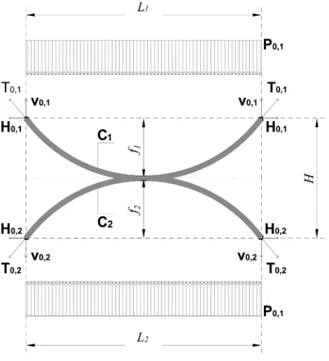
In order to create a numerical procedure, the real three-dimensional case was simplified with a two-dimensional model called “Rope beam”, like illustrated in Figure 1. The two-dimensional structural model at the base of the

proposed procedure consists of two cables with opposite curvature which have a node at midspan in common. The equilibrium of the system forces in the node in common ensures the forces transmission between the two cables.

The prefixed assumptions are: vertical links, in tension or in compression, are treated as a continuous mem-brane between the two main cables; the horizontal displacements are neglected compared to the vertical ones; pretension is considered as an equivalent distributed load; the system congruence is required only in the central span node; the mutual actions between cables are uniformly distributed as the external load, and consequently, load-bearing and stabilizing cable have a parabolic configuration also in elastic regime.

The stiffness coefficients are considered, respectively for the load-bearing cable (C1) and stabilizing one (C2)

defined as expressed in Equation (2) and Equation (3), where k1 and k2 represent, respectively, the stiffness of

the load-bearing cable C1 and the stiffness of the stabilizing cable C2, defined in Equation (4); A1 and A2, f1 and

f2, L1 and L2 are, respectively, area, sag and span length of the cable C1 and C2.

According to the iterative numerical procedure, given a fixed geometry, the external loads, the maximum stress limits and, finally, the maximum value of the forces to be transmitted to the support structures in condi-tions of maximum load applied, it is possible to compute the optimal cables area.

Cables areas are considered optimal if the cables stresses, under the maximum load design, respectively of compression and aspiration, are close to the upper and lower limit fixed in the hypothesis (σmax = 1700.0 MPa

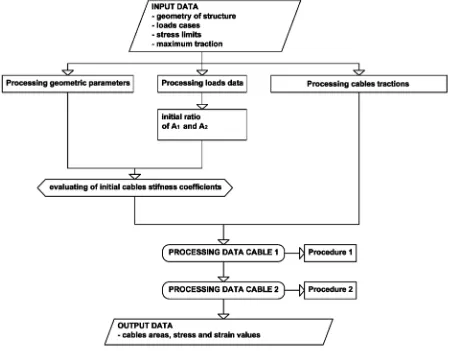
and σmin = 20.0 MPa). The global flow chart of the numerical procedure for cables net preliminary design is

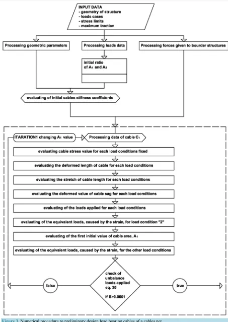
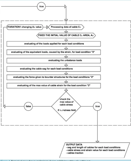
shown in Figure 2. It consist of two sub-procedures, respectively the procedure 1, illustrated in Figure 3, which allows to determine the optimum area of cable C1, and the procedure 2, illustrated in Figure 4, which allows to

compute the area of cable C2 and therefore, the balance of the applied loads, depending on the area of cable C1.

Figure 4. Numerical procedure to preliminary design stabilizing cables of a cables net.

With reference to Figure 1, the prefixed geometric quantities are the cable sags (f1 and f2) and the span length

(L1 and L2). Subscripts 1 and 2 indicate, respectively, load-bearing cables and stabilizing one. The considered

the maximum value of internal tension under the snow action, while cable C2 reaches the minimum value of

ten-sion; the cables length is modified under the load action, the initial geometry is bigger of lower in base of the direction of the load action. If the direction is gravitational the load bearing cables length increase, at contrary for the stabilizing cables. In this case, if wrongly designed, it is possible that the stabilizing cables curvature be-comes inverse and the structure bebe-comes instable. In Equations (1) and (2) the global cables stiffness Kc₁ and

2 c

K of the net is defined for the two order of cables; in Equations (4) and (5) k1 and k2 the single cables

stiffness is defined depending on the cable area, sag, span, and finally on the cable material (E is the Young Module of the cable steel assumed equal to 165,000 Mpa).

1 1 1 2 c k K k k =

+

2 2 1 2 c k K k k =

+ (3)

1

1 _{2 4}

1 1 8 32 1 3 5 EA k f f l l l =  _{   }   +  _{ } −  _{ }   _{   }    (4) 2

2 _{2 4}

2 2 8 32 1 3 5 EA k f f l l l =  _{   }   + _ _ − _ _   _{   }    (5)

The initial conditions are represented by the initial geometry, the load action considered and the material chosen in order to evaluate an initial value of cables stiffness, also a preliminary value of cables area (A0,1, A0,2)

and strain (0,1, 0,2) are fixed. This value will be iteratively modified. In Figure 3 the procedure 1 flow chart

illustrates the first step of calculus. In the following the maximum snow action strain values are named 2,1, 2,2

 and the maximum wind suction strain values are named 3,1, 3,2. The suffix “i” used in the following

eq-uations indicates the generic load condition, Gp1 is dead load, Gp2 is permanent load, S is the maximum

snow action, W is the maximum wind suction. Like a start point the ratio 1 2

k

k between the cables stiffness is

assumed equal to ∆P defined in Equation (6).

( )

( )

1 1

1 1

Load Condition 3 Load Condition 2

p p

p p

G G W

P

G G S

 + + 

∆ = =

+ +

 

  (6)

The initial geometrical cables length L0,1,geom and L0,2,geom is evaluated using the approximated formulation

reported in Equations (7) and (8), depending on cables initial sag and span.

2 4 1 1 0,1, 1 1 1 8 32 1 3 5 geom f f L L L L  _{   }    = + _{ } − _{ }        ⋅ 

⋅ ⋅ (7)

2 4 2 2 0,2, 2 2 2 8 32 1 3 5 geom f f L L L L  _{   }    = + _{ } − _{ }        ⋅ 

⋅ ⋅ (8)

The initial cables internal traction T0,1 and T0,2 is evaluated as reported in Equations (9) and (10) assumed

as the first forces of the mechanical problem; the initial horizontal traction H0,1 equal to H0,2 applied on the

boundary structures is defined in Equation (11).

2 1 0,1 0,1

1

1 16 f

T H

L  

= _{+  }

2 2 0,1 0,2

2

1 16 f

T H

L  

= _{+  }

  (10)

1 1 0,1 0 2 2 2 2 1 ,2 1 ; 8 8 p p

G L G L

H H

f f

= = (11)

The initial balance between dead load and initial fixed is assumed as first condition. The load action is applied as an uniform distribution load (named equivalent load and in the following indicated as P) on the load bearing cable. In this particular case is assumed as a hypothesis that snow action is bigger than the wind suction. The reason is that there are snow loads value in the code for each altitude but there aren’t wind loads data for Hyperbolic paraboloid shape; so the flat roof pressure coefficients is chosen as a start point. The wind load value evaluated with the flat roof pressure coefficients is general lower than the snow action for an altitude major than 200 m, using the Eurocode. In order to preliminary design the cable net for the bigger load condition at first the snow action (S) is evaluated (load condition 2). Using the procedure 1 illustrated in Figure 3, the geometry vari-ation of the load bearing cable (in this case C1) is evaluated in order to obtain the H2,1 defined by Equation (12).

It’s important to note that f2,1 and T2,1 are the deformed sag and the cable C1 traction with the snow action.

2,1 2,1 2 2,1 1 1 16 T H f L =   +    

In Equation (12) T2,1, according to the Hook law is equal to E Aε , and  and A are the strain and the cable

area that satisfy the balance in load condition 2. Replacing in Equations (2), (3), (13), (14) are defined.

( )

( )

2 2 2 2 1 1

4 4 4

1 2 2

2 1 1 4 1 1 1 1 1 1 C EA f L K

E A f E A f

EA f

P

L L L

EA f L          _{ }       _{ }          = _{ } = _{ } =    _{ +  }  _{ }  +   ∆  _{  }  _{ }       _{  + }             (13)

( )

( )

2 2 1 1 1 1 4 4 4 1 1 2 2 2 2 4 2 1 1 1 1 C EA f L K P

E A f EA f

EA f

L

L L

E A f

L          _{ }     _{ }          =  = _{ }= _{∆ + }          _{+ }         _{   }  _{ }    _{  + }               (14)

The load configuration P2,1, (load configuration 2, cable 1) that corresponds to snow action, is evaluated ac-cording to the Equation (15) obtaining by the Equations (10) and (12) and dimensionless respect the cable area

A1. It is possible to define P2,1 also according to Equation (16).

2,1 2,1 2,1 2,1 2,1

2,1 1

2 2

1 1 1

8 8

P f f

P A

A L L

ε  ε 

= ⇔ _{=  }

2,1 2,1 2,1 2

1

8H f P

L

= (16)

The relation that connect the “2” load condition and the “0” load condition is reported in Equations (17) and (18). The load balance reported in Equation (18) is obtained with an iteration of A1.

(

)

(

)

1 1

1 1 1 1

0,1 0,1 0,1

0,1 1 2 1

1 1

8

1 1

p p p p

c c

G G G G

P f

P A A

A L K K ε         +   +          =  − _{ } =  − _{ }           _{ }     _{ }   _ _   _ _      (17)

(

) (

)

( )

1 1 1 1

0,1 2,1

0,1 0,1 2,1 2,1 1

1 1 0,1

2 2

1 1

iteration

1 1

8 8

0 to , fixed a 1

p p p p

c c

c

G G S G G

P P

K K

f S f A

A A L L K ε ε ε       + + +    ∆ =_ +_ − _−       _{   }    _ _ _ _                     − − =      _{ }          _{ }  _{ }  =   

(

)

(18)

With the same procedure A2 is fixed updating the value of A1. In conclusion, fixed an initial condition of

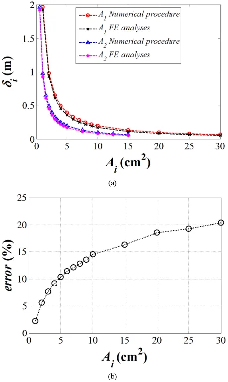
traction the cables areas are defined according to the initial geometry wanted. In Figures 2-4 the flow charts of the procedure described are shown in order to summarize step by step the numerical proceedings. To validate the numerical procedure a comparison of the cables structural response with a Finite element method analyses (in the following FE) is done; in Figure 5(a) and Figure 5(b) the vertical displacements of the middle node is plotted for different cables areas but with same load applied (in this case equal to 2.2 kN/m gravitational and uniform load on the load bearing cable). The load bearing cable sag and span are equal to 4.44 and 80 m, the

stabilizing cables sag and span are equal to 8.89 and 80 m; in this case the ratio 1 2

A

A is assumed equal to 2. The

mean value of the percentage error is equal to 12%. This value appear acceptable if the approximation is consi-dered. In the following the numerical procedure described in this section will be named NPPD (Numerical Pro-cedure of Preliminary Design) (Elashkar I., Novak M., 1983; Lewis W. J., 2004; Majowiecki M., 2004) [8]-[10].

2.2. The Analyzed Geometric Sample

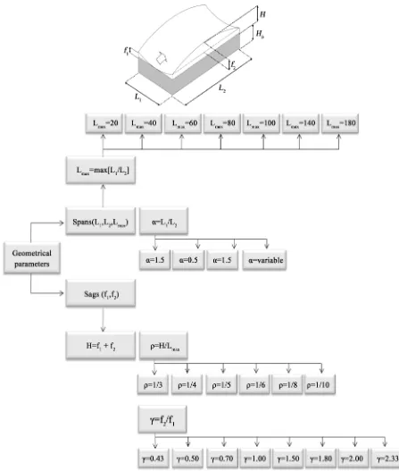
In order to estimate a set of optimal geometry with the minimum cables areas and displacements (for equal forces transmitted to the support structure) [11]-[15], a geometric parameterization taking into account the fol-lowing parameters was carried out (Figure 6):

• γ, the relationship between the cable sags, (f2/f1); 8 different values of γ, respectively equal to 0.43, 0:50, 0.70,

1.00, 1.50 1.80, 2.00, 2.33 were taken into account;

• ρ, the relationship between the roof height and the maximum span length (H/Lmax); 6 different values of ρ,

respectively equal to 1/3, 1/4, 1/5, 1/6, 1/8, 1/10 were taken into consideration.

• α, the relationship between the span length (L1/L2); 4 different values of α, respectively equal to 1.50

(rec-tangular plan shape), 1.00 (square plan shape), 0.50 (rec(rec-tangular plan shape), and variable, for structures with a circular plan shape were taken into account.

With the previously numerical procedure, 1008 different geometrical combinations were analyzed; only some configurations meet the optimization criteria pre-fixed in the hypotheses; in particular:

• Cables net with L1 < L2 show better performance with lower values of forces transmitted to the supports.

weight.

• “Optimal” values of γ, both as regards stress and structural weight optimization, are in the range between 1.5 and 2.5.

• Low values of ρ give higher cables areas and therefore a higher structural weight; however, they gives “op-timal” stresses with respect to cables net with high value of ρ.

• The ratio between the obtained displacements with lower span lengths and those obtained with higher spans are lower compared to a direct proportionality.

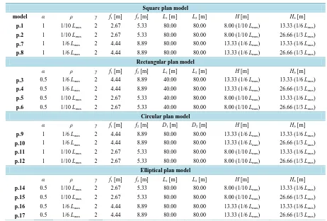
Totally one thousand geometries are investigate in order to compare the structural response and to choose an optimal sample to test in wind tunnel. On the basis of these preliminary results, a representative geometric sam-ple to be tested in the wind tunnel was chosen; in Table 1 the geometrical sizes of the full scale cable nets are listed for each plan shape. This phase of the work has produced a preliminary design numerical procedure with which it is possible to identify the sample to test in wind tunnel. A model scale equal to 1:100 is chosen to con-struct the models.

3. Numerical Procedure to Generate Cables Net Fe Models

Before wind tunnel test, tridimensional FE analyses are performed in order to simulate examples of full scale structures. The weight of the cables nets and their structural response under the snow action are studied to verify that the geometries chosen give a high structural response. In order to provide the geometric input for FEM models

(a)

(b)

Figure 6. Geometrical configurations investigated with the numerical procedure for cables net preliminary design.

Table 1.Geometrical sample.

Square plan model

model α ρ γ f1 [m] f2 [m] L1 [m] L2 [m] H [m] Hb[m]

p.1 1 1/10 Lmax 2 2.67 5.33 80.00 80.00 8.00 (1/10 Lmax) 13.33 (1/6 Lmax)

p.2 1 1/10 Lmax 2 2.67 5.33 80.00 80.00 8.00 (1/10 Lmax) 26.66 (1/3 Lmax)

p.7 1 1/6 Lmax 2 4.44 8.89 80.00 80.00 13.33 (1/6 Lmax) 13.33 (1/6 Lmax)

p.8 1 1/6 Lmax 2 4.44 8.89 80.00 80.00 13.33 (1/6 Lmax) 26.66 (1/3 Lmax)

Rectangular plan model

α ρ γ f1 [m] f2 [m] L1 [m] L2 [m] H [m] Hb [m]

p.3 0.5 1/6 Lmax 2 4.44 8.89 40.00 80.00 13.33 (1/6 Lmax) 13.33 (1/6 Lmax)

p.4 0.5 1/6 Lmax 2 4.44 8.89 40.00 80.00 13.33 (1/6 Lmax) 26.66 (1/3 Lmax)

p.5 0.5 1/10 Lmax 2 2.67 5.33 40.00 80.00 8.00 (1/10 Lmax) 13.33 (1/6 Lmax)

p.6 0.5 1/10 Lmax 2 2.67 5.33 40.00 80.00 8.00 (1/10 Lmax) 26.66 (1/3 Lmax)

Circular plan model

α ρ γ f1 [m] f2 [m] D1 [m] D2 [m] H [m] Hb[m]

p.9 1 1/6 Lmax 2 4.44 8.89 80.00 80.00 13.33 (1/6 Lmax) 13.33 (1/6 Lmax)

p.10 1 1/6 Lmax 2 4.44 8.89 80.00 80.00 13.33 (1/6 Lmax) 26.66 (1/3 Lmax)

p.11 1 1/10 Lmax 2 2.67 5.33 80.00 80.00 8.00 (1/10 Lmax) 13.33 (1/6 Lmax)

p.12 1 1/10 Lmax 2 2.67 5.33 80.00 80.00 8.00 (1/10 Lmax) 26.66 (1/3 Lmax)

Elliptical plan model

α ρ γ f1 [m] f2 [m] L1 [m] L2 [m] H [m] Hb [m]

p.14 0.5 1/10 Lmax 2 2.67 5.33 80.00 80.00 8.00 (1/10 Lmax) 13.33 (1/6 Lmax)

p.15 0.5 1/10 Lmax 2 2.67 5.33 80.00 80.00 8.00 (1/10 Lmax) 26.66 (1/3 Lmax)

p.16 0.5 1/6 Lmax 2 4.44 8.89 80.00 80.00 13.33 (1/6 Lmax) 13.33 (1/6 Lmax)

p.17 0.5 1/6 Lmax 2 4.44 8.89 80.00 80.00 13.33 (1/6 Lmax) 26.66 (1/3 Lmax)

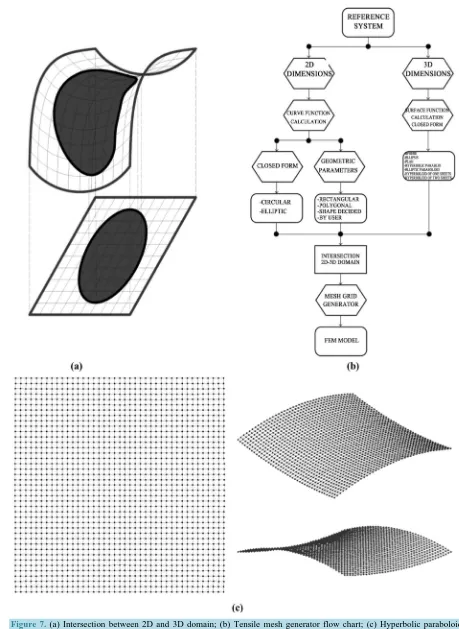
importing a.dxf (Drawing Interchange Format) file that describes the two-dimensional domain or, in the case of complex and irregular domains, it is possible to directly import the coordinates of the shape vertices. After set-ting the two-dimensional domain, the three-dimensional one can be set by choosing among seven prefixed shapes (sphere, ellipsoid, flat, hyperbolic paraboloid, elliptic paraboloid, a one slope hyperboloid and a two slopes hyperboloid). Also in this case it is possible to directly insert geometric parameters and surfaces coeffi-cients, or compute their functions through an equations system obtained by setting some points coordinates on the surface. The next step concern the insertion of the cables spacing in the two directions, X and Y in the case of Cartesian coordinates, or meridians and parallels in the case of polar coordinates. In the case of Cartesian system, the procedure computes the equation of each line that describes the cable, and then intersects lines with the 2D domain generating a set of nodes and computing the respective coordinates on the plane, pi(xp, yp). In the next

step the procedure projects the evaluated nodes on the spatial surface, identifying the third coordinate zp.

In the exporting phase, 3 different files can be saved: a.txt (text file) for input that contains the number of nodes and their coordinates; a.dxf with the cables net vector model; and a file that contains the functions equa-tions of the created curves and surfaces. Thanks to this procedure, FEM model for nonlinear dynamic analyses can easily be generated. Figure 7(a) shows the intersection between the 2D domain and the 3D domain, while

Figure 7(b) shows the simplified flow chart of the numerical procedure. Finally, in Figure 7(c) an example of hyperbolic paraboloid mesh with square plan shape generated is reported. Static and modal FE analyses are per-formed using the numerical models tested. Using the .dxf files generated the wind tunnel models are constructed made of wood. In the following the numerical procedure described in this section will be named Numerical Procedure to Generate Finite Element Models, in the following NPGFM[16]-[18].

4. Wind Tunnel Test

4.1. Setup

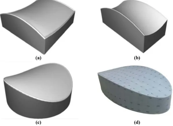
air moving past solid objects rigid and flexible. A wind tunnel consists of a tubular passage with a particular geometry where the object to test is in the middle of the test chamber. Air is made to move past the object by a powerful fan system or other means. The wind tunnel model is instrumented with suitable sensors to measure aerodynamic forces, pressure distribution, or other aerodynamic-related characteristics. In this experience the models are rigid and the goals were to acquire pressure coefficients [19]-[25].

The CRIACIV (Inter-University Research Center for Building Aerodynamics and Wind Engineering) wind tunnel located in Prato (Italy) is used to perform aerodynamic experiments. A layout of the wind tunnel is illu-strated in Figure 8. The choice of the turbulence intensity and so of the wind tunnel speed profile is important, too. For this research a more general possible condition was necessary. A medium urban profile is chosen for the boundary layer. In Figure 9(a) and Figure 9(b) the boundary layer development artificial roughness (wood pa-nels) (a), spires (b) are shown and in Figure 9(c) and Figure 9(d) the speed and turbulence profile is reported. The mean value of the wind tunnel speed at the roof level is between 16 and 20 m/s, the turbulence at the same level is between 12% and 15% (Simiu E., Scanlan, R. H., 1986).

The test models are made in wood and their geometrical scale is fixed equal to 1:100; the reason of this choice is to have big models and so easy to construct but with a not much high blockage coefficients. The constructions follows the geometry designed using the numerical procedure described in Section 3. Test models pictures are shown in Figure 10, respectively with a square plan (a), rectangular plan (b), circular plan (c) and elliptical plan (d). The geometry of the wind tunnel models is described in Table 1. Each model was instrumented (Figure 11(a) and Figure 11(b)) varying from 175 to 211 pressure taps distributed on the roof like shown in Figure 11(c). Each pressure tap was connected to a pressure transducers with a pneumatic connection made of Teflon tubes with 1.3 mm internal diameters (Figure 11(a) and Figure 11(b)). Data for 16 different wind angles were acquired at a frequency of 252 Hz and for 30 seconds obtaining, for each pressure tap, a pressure time history of 7504 values.

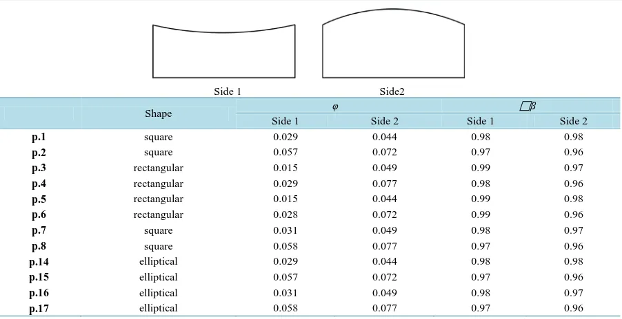
The ratio between the models size and the test chamber section size is very important (φ). If this ratio is big (2% or 3%) the blockage effects increases pressure coefficients and correction factors are necessary. In this case the blockage effect is not negligible and so a blocking coefficient β was considered. According to Equation (19)

φ is evaluated and the correction factor β is estimate. Atot is the wind tunnel test section area and Alateral is the

model section area.

2 tot lateral

tot

A A

A ϕ=  − 

  (19)

In Table 2 blockage values and the correction coefficients for each tested model are reported. They are in a range between 1.5% and 7.7% with peaks for geometries p.2, p.4, p.6, p.8, p.15 and p.17 (highest model). The correction values for the pressure coefficients vary from a minimum of 2% to a maximum of 4%.

Figure 9. Boundary layer development artificial roughness (wood panels) (a), spires (b); (c) velocity and (d) turbulence pro-files.

Figure 11. Wind tunnel acquisition data, (a) and (b) model instrumentation, (c) example of pressure taps distribution.

Table 2.Blockage values.

Side 1 Side2

Shape φ β

Side 1 Side 2 Side 1 Side 2

p.1 square 0.029 0.044 0.98 0.98

p.2 square 0.057 0.072 0.97 0.96

p.3 rectangular 0.015 0.049 0.99 0.97

p.4 rectangular 0.029 0.077 0.98 0.96

p.5 rectangular 0.015 0.044 0.99 0.98

p.6 rectangular 0.028 0.072 0.99 0.96

p.7 square 0.031 0.049 0.98 0.97

p.8 square 0.058 0.077 0.97 0.96

p.14 elliptical 0.029 0.044 0.98 0.98

p.15 elliptical 0.057 0.072 0.97 0.96

p.16 elliptical 0.031 0.049 0.98 0.97

4.2. Data Processing

Experimental data consist in pressure expressed in mmH2O deriving by the transducers acquisition; a numerical

procedure is needed in order to obtain a double goal: at first pressure in Pascal and pressure coefficients located on the roof and at second, forces time history to use in FEM analysis. For this reason a numerical procedure have to transform data into pressures, then evaluate the pressure coefficients, then estimate the maximum, min-imum and mean values of these coefficients, and finally transform the pressure coefficients into forces to be ap-plied on the FEM model. The first phase concerns the graphic aspect, with the preparation of the geometry of the pressure coefficients map; the second stage involves the implementation of the subroutine for the evaluation of the pressure coefficients and the third phase provides the forces calculation.

4.2.1. Pressure Coefficients Maps

In order to obtain pressure coefficients maps to describe the pressure distribution on the roof and sides of the model, the surface was discretized in polygons surrounding each pressure taps. The Thiessen (Voronoi) poly-gons theory is adopted. It consists to define individual areas of influence around each of a set of points. Thiessen polygons are polygons whose boundaries define the area that is closest to each point relative to all other points.

They are mathematically defined by the perpendicular bisectors of the lines between all points. The process goes through several steps: collects the points from a point layer (vertices if the source is a polyline or polygon layer), clean duplicate points, generates Convex Hull, creates a TIN structure, generates perpendicular bisectors for each tin edge, builds the Thiessen polygons and, finally, clips the Thiessen polygons feature class with the convex hull. A specific numerical procedure is programmed for this section. An example of Thiessen polygons distribution is illustrated in Figure 12. It is possible to note that if the pressure taps distribution is not geometri-cally regular with a structured grid, the shape of the Thiessen polygon is irregular. For each polygon one value of pressure coefficient is associated [19]-[25].

4.2.2. Evaluation of Pressure Coefficients

During wind tunnel tests the model is fixed in the test chamber, in Figure 13(a) a picture of a model during the test is shown. The tubes connected to the transduces sent an input to the computer that measure the pressure variation in mm H2O. The experimental data needs to be transformed in pressure coefficients. Pressure

coeffi-cients (Cp), is a dimensionless number which describes the relative pressures throughout a flow field in fluid

Figure 13.(a) Model in the wind tunnel; (b) Pressure coefficients map (mean values); (c) Pressure coefficients 3D mesh; (d) Typical forces time history.

dynamics; it is evaluated by the ratio between the difference of the local pressure and the undisturbed flow pressure, and undisturbed dynamic flow pressures are evaluated for each wind direction. Maximum (Cp,max),

minimum (Cp,min) and mean values (Cp,m) of the pressure coefficients are extracted from the obtained pressure

In the following the numerical procedure described in this section will be named NPWDP (Numerical Proce-dure for the Wind tunnel Data Process).

4.2.3. Data Exchange between Wind Tunnel and FEM Analysis

In order to use experimental data to perfume FEM analyses, the same surface discretization between wind tunnel test model and FE model is necessary. Often that is impossible because the number of pressure taps used for each models is generally less than the FE model nodes. Also in this case it was happened. The mean value of pressure taps number used on the roof is 90, the number of nodes used in FEM analysis to describe the cable net is about 1700. A numerical procedure to extend the experimental data on the FEM mesh is necessary. There are to more used possibilities: the first is obtained overlapping the FEM mesh and the Thiessen polygons distribu-tion, the same pressure coefficient is used for all FEM nodes that are surrounding by polygon. A second way is to estimate a mathematical procedure to interpolate the experimental data respect the FEM mesh. Both proce-dures were implemented. The first solution follows the following sequence: the polygons edges coordinates (Cartesian reference system) are determined; a scan of the FEM nodes coordinates is been done in order to check the proximity from the polygon edge. The nodes that have coordinates between the polygon minimum and maximum coordinates are in the polygon. The second procedure is more difficult. The first phase is the same to the previous solution, but during the scan a value of pressure coefficients for each node is assumed; the values is evaluated using the inverse distance weight (IDW) interpolation method (Borrough P.A., 1986; Greville T.N.E., 1969; Hohn M.E. (editor), 1998). An example of 3-dimensional pressure coefficients map obtained using this last method is shown in Figure 13(c). Using the pressure coefficients time history assumed for each FEM nodes, a wind loads time history is evaluate. In this case in order to obtain the structural response of a cable net under wind action, a localization of the net is necessary. A value of wind kinetic pressure and geographical aspects are chosen. A preliminary ramp is added by the load history, it has a length equal to about 1% of the history length. In Figure 13(d) an example of the load history is shown for a cable net center point (N1) (Shen S., Yang Q. 1999). In the following the numerical procedure described in this section will be named NPED (Numerical Pro-cedure to Exchange Data). In Figure 14 the procedure is summarized [16]-[18].

5. Wind-Structure Interaction with Time History Analysis

In order to estimate cables nets structural response, Nonlinear Dynamic Analyses have to be performed. The analyses are conducted on the tested sample using numerical procedures implemented by Full Professor PieroD’Asdia staff; the procedures are merged in a main program in the following named TENSO. It isn’t a commercial software and it was born as a set of numerical procedures and subroutines merged step by step from 1980. The description of these procedures has never been published.

The Non Linear Structural Analysis Program

inertia along the beam axis with a polynomial function. In order to evaluate the stiffness matrix, a numerical procedure based on the validity of the constitutive elastic low is used and six independent functions to describe the displacement field is used, too. At the beginning, the procedure computes the flexibility matrix of the ele-ment, applying a forces system and evaluating a displacement system using an algorithm that, step by step, computes the twelve conditions of kinematic compatibility and the balance evaluated in the previous step. The Gauss method is used for the numerical integration and Rayleigh damping is implemented. In the case investi-gated a value of 1% of structural damping is used; the value is in line with literature references. TENSO soft-ware simultaneously uses two solution methods to solve nonlinear analysis: the step by step incremental method and the interaction progressive method with the variable stiffness matrix as well as the secant method. The se-cant method can be thought of as a finite difference approximation of Newton's method.

In TENSO, secant method is used as a check method that permits to stop the analysis with a unbalanced solu-tion. Using the step by step incremental method, nonlinear problem can be transformed in a succession of linear problems. Each calculation step stores loads and strains history evaluated during the previous step. For each analysis step, a small enough part of load (ΔP) necessary to ensure that is possible to use the elasticity method is applied. However, this simple and classical approach presents the difficulty to evaluate the exact dimension of load step and so the exact step of analysis. A non-appropriate chosen range can cause an inexact solution. In or-der to solve it, TENSO uses the method with the variable stiffness matrix; this method is a vector version of the Newton-Raphson modified method about nonlinear equation systems. The Newton-Raphson procedure guaran-tees convergence if and only if the solution at any iteration is close to the exact solution. Therefore, even without a path-dependent nonlinearity, the incremental approach (i.e., for subsequent load steps) is sometimes required in order to obtain a solution corresponding to the final load level. If the displacements are large, the product be-tween the stiffness matrix, evaluated on the basis of the solution of the previous step and on the basis of the stresses, and the displacements vector, give the internal force vector, not equilibrate with the external forces vector according to Equation (20), where K is the stiffness matrix, δ is the displacements vector, P is the external forces vector; the difference between these two forces vectors represents the imbalance force vector, according to Equation (21), where R is the residual vector and P is the internal forces vector. In the following step, this vector is applied as an external load modifying the displacement vector with a residual value of dis-placements, according to Equation (22) where Δδ is residuals values of displacements to update the geometry, and so updating the structure geometry.

[ ]

{ }

{ }

[ ]

{ }

{ }

 

=_ −  _≠ (21)

{ }

[ ]

{ }

1 1 1

Δδ _k+ = K _k−₊ R _k+ (22)

gram of the numerical procedures described in this section in the following will be named NPSA.

6. Applications

In order to demonstrate the validity of the procedure, two examples of different structures covered with cables net are described: the first one is a project proposal under review (2012) of a roller skates arena and the second is basketball arena; the last one is a project proposal for the renovation of an existent sports arena (2007).

6.1. Project of a Roller Skates Arena

The building designed is located in Pescara, middle Italy, and its purpose is to cover an existent open space used for roller skates competitions (Rizzo et al., 2014). The building has a circular plan and is covered with an Hyperbolic Paraboloid cables net roof. The most important geometrical parameters are summarized in Table 2. The horizontal traction (referring to Equation (11)) is absorbed by a series of external pillars and beams located around the building like are illustrated in Figure 17(c). In Figure 17(a) a global view of the urban contest and in

Figure 17(b) a significant plan of the building are shown. The geometry chosen is one of the optimal geometries studied and described in Figure 16 and obtained by the procedure described in Section 2. In this phase of the project wind tunnel experiments results obtained with the parametric study described in Section 3 are sued. Of course after this first preliminary phase some specific wind tunnel experiments are necessary to study aerody-namic and aeroelastic effects. The pressure coefficients maps (Rizzo et al., 2011 and Rizzo, 2014) for two sig-nificant angles used to evaluate the wind action are shown in Figure 18. The wind direction of 0˚ are parallel to

the stabilizing cables and at contrary, the wind direction of 90˚ are parallel to the load bearing cables.

A FEM model is analyzed and geometrical non-linear analyses are carried out in order to design the structural components of the building. The procedure described in Section 3 is followed to define the FEM models and some pictures are illustrated in Figure 19. The mechanical parameters are reported in Table 3, where D is the externa diameter of the building, A1and A2 are respectively the load bearing cables and the stabilizing cables, ε1

Figure 17. External views of the roller skates arena

and ε2 are the strains cables for the load configuration number 1 (according to Section 2); Hb is the drum high of

the building, H is equal to the f1 + f2.

Using the numerical procedure described in Section 4, nonlinear analyses are carried out in order to study at first the structure deformation and its natural frequencies. Modal analyses and then a dynamic time history anal-ysis are permed using the wind tunnel experiments results. Some results are illustrated in Figure 20 and Figure 21. In particular the first 9 modes shape are reported in Figure 20 and are listed in Table 4, the deformation un-der 0 wind action is reported in Figure 21. Observing the cables area values reported in Table 3 and considering that 40 load bearing cables and 40 stabilizing cables are used, we note that the structural weight of the roof is re-ally low, the cables net weight is only 1.5 × 10−2 kN to square meters. One aspect ore is important to note: the first 9 modes are totally roof’s mode and the periods are very high. This structures are particularly optimal in seismic zones because are flexible and ductile.

6.2. Project of a Basketball Arena

(a)

(b)

Figure 19. FEM models views.

Table 3. Geometrical and mechanical parameters.

f1 (m) f2 (m) D (m) H (m) Hb(m) A1 (cm2) A2 (cm2) ε1 (‰) ε2 (‰)

2.67 5.33 80.00 8.00 13.33 7.89 3.93 11.45 5.13

Table 4. Natural frequencies and periods.

Mode Frequency (Hz) Period (s)

1 0.149 6.679

2 0.179 5.584

3 0.215 4.647

4 0.244 4.099

5 0.254 3.933

6 0.293 3.417

7 0.296 3.377

8 0.313 3.190

9 0.340 2.939

10 0.352 2.844

Figure 21. Upward deformation under 0˚ wind action.

building renovation was the championship European basketball competition (2007) (Rizzo et al., 2012). The proposal is being evaluated by the municipality government for the future renovation.

The idea is to realize an external structure with a square plan in order to have a total open space into the arena. Some pictures of the actual structure and the future modification are illustrated in Figure 22. A square plane is chosen in order to respect the actual shape of the building and its urban contest. A series of stays are used to ab-sorb the horizontal traction of the cables net, like is shown in Figure 22. In Table 5 the main geometrical para-meters are listed and the cables areas and strains for the load configuration number 1 (according to Section 2).

The structural response is evaluated with Non-Linear analyses carried out with a FEM model modelled with the numerical procedure described in Section 3. Some pictures of the FEM model are shown in Figure 23. Us-ing the numerical procedure described in Section 5 the Natural frequencies and displacements under loads com-binations are evaluated, too. In Figure 24 the first 10 modes shape deformations are reported and in Table 6

their values are listed. It’s interesting to note that the period is higher than the other geometry described in Sec-tion 7.1; it’s caused by many reason, at first the plan geometry because the circular shape gives a more rigid border structure, at second the cables areas and strains are lower for this geometry, finally, this structure is also higher than the previous.

The wind action is applied on the FEM model like a series of time histories evaluated by wind tunnel experi-ments and a dynamic analysis is performed. In Figure 25 a view of the structure deformation under 90˚ wind

the structural response in term of cables strains, traction and deformation variation, is reported; T1 and T2 are the

cables traction evaluated according to the Equation (10), Δf is the sag variation.

7. Conclusion

Every time that an experiment is processed, a great number of numerical procedures are programmed by re-searcher to control the process. These numerical procedures are often isolated and programmed again for every different case of study. An interesting goal is to create a free open domain where the numerical procedures eva-luated are merged, added, modified by researchers with the aim to obtain a common space of use. With this purpose, the present paper described a methodology followed to prepare a wind tunnel test and to process results. Five different steps NPPD → NPGFM → NPWDP → NPED → NPSA give a one complete numerical proce-dure that can be expanded, modified or completed by everyone. In this specific case the subroutines can be modified to capture more and more different geometries or structural typologies with the aim to obtain a globa-lized virtual space of calculus. This paper is focused to wind tunnel tests because they are generally complex,

Figure 22. (a) External view of the actual structure; (b) Future modification of the building.

Table 5.Geometrical and mechanical parameters.

f1(m) f2(m) L1(m) L2(m) H (m) Hb(m) A1(cm2) A2(cm2) ε1(‰) ε2(‰)

4.44 8.89 80.00 80.00 13.33 13.33 5.71 2.31 6.70 7.60

Figure 24. Modes shape deformation.

Table 6. Natural frequencies and periods.

Mode Frequency (Hz) Period (s)

1 0.132 7.563

2 0.154 6.509

3 0.165 6.068

4 0.180 5.566

5 0.180 5.552

6 0.202 4.944

7 0.208 4.807

8 0.233 4.299

9 0.228 4.386

10 0.247 4.047

Figure 25.Upward deformation under 90˚ wind action. Table 7. Structural response.

1 (‰) 2 (‰) T1 (KN) T2 (KN) Δf (m)

max min max min max min max min max min

Comb.1 (Permanent loads) 6.75 5.43 9.63 6.29 635.95 511.59 367.05 239.74 −0.10 −3.4 × 10−5

Comb.2 Snow 7.92 5.97 9.16 5.87 746.18 562.46 387.25 71.28 −0.92 −1.0 × 10−3 Comb.3 Wind 0˚ 6.00 4.85 9.86 6.98 659.51 456.94 375.81 266.04 0.36 1.7 × 10−4 Comb.3 Wind 90˚ 5.78 3.92 10.14 6.87 657.62 463.83 386.87 262.04 0.30 1.5 × 10−4

processing data procedure permits to evaluate the experimental data and to prepare the input of the FEM analys-es. Finally, the nonlinear structural analyses procedure permits to evaluate the structural response. The global flow chart is illustrated in Figure 16.

Acknowledgements

Special thanks to Full Professor PieroD’Asdia for the research coordination, to Engineer Massimiliano Lazzari for his for his collaboration in the planning process described in Section 2, to Engineer Fabrizio Fattor for his collaboration in the planning process described in Section 3, to Associate Professor Gianni Bartoli and the CRIACIV Wind tunnel boundary layer staff, in particular Engineer PhD Tommaso Massai and Lorenzo Procino, for the coordination of the wind tunnel tests and the numerical procedure programming described in Section 4, to Architect PhD Federica Speziale for the FEM analysis described in Section 5, finally to PieroD’Asdia, Fabri-zioFattor, Salvatore Noè and Luca Caracoglia for the calculation program described in Section 5.

References

[1] Rizzo, F. (2014) Aerodynamic of Tensile Structures. Silvana Editoriale, Milan.

[3] Rizzo, F., D’Asdia, P., Ricciardelli, F. and Bartoli, G. (2012) Characterisation of Pressure Coefficients on Hyperbolic Paraboloid Roofs. Journal of Wind Engineering & Industrial Aerodynamics, 102, 61-71.

http://dx.doi.org/10.1016/j.jweia.2012.01.003

[4] Rizzo, F. (2012) Wind Tunnel Tests on Hyperbolic Paraboloid Roofs with Elliptical Plane Shapes. Engineering Struc-tures, 45, 536-558. http://dx.doi.org/10.1016/j.engstruct.2012.06.049

[5] Rizzo, F., D’Asdia, P. and Speziale, F. (2012) FEM Analysis of Tension Structures with Experimental Wind Action. The 2012 International Conference on Advances in Wind and Structures (AWAS’12), Seoul, 26-30 August 2012, 3373- 3381.

[6] Rizzo, F. and Sepe, V. (2015) Static Loads to Simulate Dynamic Effects of Wind on Hyperbolic Paraboloid Roofs with Square Plan. Journal of Wind Engineering & Industrial Aerodynamics, 137, 46-57.

http://dx.doi.org/10.1016/j.jweia.2014.11.012

[7] Rizzo, F., D’Asdia, P. and Speziale, F. (2014) Design of Hyperbolic Paraboloid Roofs with Circular and Elliptical Plan Shape. 13th National Conference of Wind Engineering, Geneva, 22-25 June 2014.

[8] Lewis, W.J. (2004) Tension Structures: Form and Behaviour. ASCE Standard.

[9] Majowiecki, M. (2004) Tensostrutture: Progetto e Verifica. Edizioni Crea, Milano. (In Italian)

[10] Melchers, R.E. (1987)Structural Reliability. Elley Horwood Ltd., UK.

[11] ASCE (American Society of Civil Engineers) (2005) Minimum Design Loads for Buildings and Other Structures. ASCE 7-05.

[12] Australian/New Zealand Standard (2002) Structural Design Actions; Part 2: Wind Actions. AS/NZS 1170.2:2002.

[13] Borrough, P.A. (1986) Principles of Geographical Information Systems for Land Resources Assessment. Oxford Uni-versity Press, Oxford.

ESRI (1996) ArcView Spatial Analyst Manual (Ver. 3.0).

[14] CNR (National Research Council of Italy) (2011) CNR-DT 207/2008—Guide for the Assessment of Wind Actions and Effects on Structures.

[15] CEN (Comité Européen de Normalisation) (2005) EN 1991-1-4: Eurocode 1: Actions on Structures—Part 1-4: General Actions—Wind Actions.

[16] Crisfield, M.A. (1991) Non-Linear Finite Element Analysis of Solids and Structures. Vol. 1, John Wiley & Sons, Ho-boken.

[17] Greville, T.N.E., Ed. (1969) Theory and Applications of Spline Functions. Proceedings of an Advanced Seminar, Madison, 7-9 October 1968, Academic Press, New York.

[18] Smith, I.M. and Griffiths, D.V. (1982) Programming the Finite Element Method. John Wiley & Sons, Hoboken.

[19] Cook, N.J. and Mayne, J.R. (1979) A Novel Working Approach to the Assessment of Wind Loads for Equivalent Static Design. Journal of Wind Engineering & Industrial Aerodynamics, 4, 149-164.

http://dx.doi.org/10.1016/0167-6105(79)90043-6

[20] Cook, N.J. and Mayne, J.R. (1980) A Refined Working Approach to the Assessment of Wind Loads for Equivalent Static Design. Journal of Wind Engineering & Industrial Aerodynamics, 6, 125-137.

http://dx.doi.org/10.1016/0167-6105(80)90026-4

[21] Elashkar, I. and Novak, M. (1983) Wind Tunnel Studies of CABLE ROOFS. Journal of Wind Engineering & Industri-al Aerodynamics, 13, 407-419. http://dx.doi.org/10.1016/0167-6105(83)90160-5

[22] Gumbel, E.J. (1958) Statistic of Extremes. Columbia University Press, Columbia.

Mayne, J.R. (1978) On Design Procedures for Wind Loading. Building Research Establishment, Garston.

[23] Gumbel, E.J. (1958) Statistic of Extremes. Columbia University Press, Columbia.

Lieblein J. (1974) Efficient Methods of Extreme Value Methodology. Report 74-602, National Bureau of Standards, Washington DC.

[24] Shen, S. and Yang, Q. (1999) Wind-Induced Response Analysis and Wind-Resistant Design of Hyperbolic Paraboloid Cable Net Structures. International Journal of Space Structures, 14, 57-65.

http://dx.doi.org/10.1260/0266351991494696