Using a finite horizon numerical optimisation method for a periodic optimal control problem

Munich Personal RePEc Archive

Using a finite horizon numerical

optimisation method for a periodic

optimal control problem

Azzato, Jeffrey D. and Krawczyk, Jacek

Victoria University of Wellington

11 February 2007

Online at

https://mpra.ub.uni-muenchen.de/2298/

USING A FINITE HORIZON NUMERICAL OPTIMISATION METHOD FOR A PERIODIC OPTIMAL CONTROL PROBLEM

JEFFREY D. AZZATO & JACEK B. KRAWCZYK

Abstract. Computing a numerical solution to a periodic optimal control

problem is difficult. A method of approximating a solution to a given (sto-chastic) optimal control problem using Markov chains was developed in [3]. This paper describes an attempt at applying this method to a periodic optimal control problem introduced in [2].

2007 Working Paper

School of Economics and Finance

JELClassification: C63 (Computational Techniques), C87 (Economic Software).

AMS Categories: 93E25 (Computational methods in stochastic optimal control).

Authors’ Keywords: Computational economics, Approximating Markov decision chains.

This report documents 2007 research into Computational Economics Methods

directed by Jacek B. Krawczyk

supported by University Research Fund, GMS Grant Number 16378.

Correspondence should be addressed to:

Contents

Introduction 1

1. Periodic Optimal Control Problem 1

1.1. Problem Formulation 1

1.2. Remarks on Analytical Solution 2

2. Solution withSOCSol4L 3

2.1. About SOCSol4L 3

2.2. Solution Syntax 3

2.3. Results 5

2.4. System Specifications and Computation Time 8

Introduction

In [2], Gaitsgory and Rossomakhine develop a numerical method for approximating a solution to a long run average problem of optimal control via linear programming. They consider optimal control problems of the form:

inf (u(·), y(·))

1

S

Z S 0

g(u(τ), y(τ))dτ

(1)

subject to:

˙

y(τ) =f(u(τ), y(τ)) (2)

where:

• f :U_×Rm →Rm is continuous in (u, y) and satisfies Lipschitz conditions iny,

• The controls are Lebesgue measurable functions u : [0, S] _→ U and U is a compact metric space, and

• The infimum in (1) is taken over all admissible pairs (u(_·), y(_·)) on [0, S]. A pair (u(τ), y(τ)) is said to be admissible on [0, S] if (2) holds for almost all τ _∈ [0, S] and (_∀τ _∈[0, S])y(τ)_∈Y, where Y is a given compact subset ofRm.

If the infimum is taken over only those admissible pairs that are periodic, i.e.such that:

(_∀τ >0) (u(τ), y(τ)) = (u(τ+T), y(τ +T))

for someT >0, then (1) becomes a periodic optimisation problem of the form:

(3) inf

(u(·), y(·)) 1

T

Z T 0

g(u(τ), y(τ))dτ

where the infimum is now taken overT and all admissible pairs defined on [0, T] that satisfy the periodicity conditiony(0) =y(T).

In this paper, we show how SOCSol4L(see [1]) can be used to solve a periodic optimal control problem of this type.

1. Periodic Optimal Control Problem

1.1. Problem Formulation. We examine Example 1 of [2]. In this example, Gaitsgory and Rossamakhine take:

g(u, y) :=u2₋y₁2

(4)

and

in (3) and (2) respectively, where y := (y1, y2) and U := [−1,1]. Note thatf results from the reduction of the differential equation:

¨

x(τ) +₁₀3x˙(τ) + 4x(τ) =u(τ)

to a first order system.

1.2. Remarks on Analytical Solution. This problem may be investigated analytically with the aid of, for example, the Maximum Principle. While we shall not attempt a full analytical solution here, it is instructive to consider how one might proceed.

The (simple) Hamiltonian for the problem is:

H(u, y, π) : =₋g(u, y) + 2 X

i=1

πifi(u, y)

=y₁2₋u2+π1y2+π2(−4y1−₁₀3y2+u)

So the optimal control is:

ˆ

u:= arg max

u H(u, y, π)

Clearly:

(6) uˆ(τ) =

        

1 ifπ2(τ)>2

π2(τ)

2 if|π2(τ)|<2

−1 ifπ2(τ)<−2

It follows that the optimal solution exhibits a “bang-bang control with a transition”. The system of adjoint equations for the problem is:

˙

π(τ) = "

−∂H(∂yu,y,π1 )

−∂H(∂yu,y,π2 ) #

= "

−2y1+ 4π2

−π1+ ₁₀3π2 #

Combining these with the state evolution ˙y=f(ˆu, y) yields the canonical system:

(7) d dτ       y1 y2 π1 π2       =      

0 1 0 0

−4 ₋₁₀3 0 0

−2 0 0 4 0 0 ₋1 ₁₀3

            y1 y2 π1 π2       +       0 ˆ u 0 0      

Solving this when_|π2(τ)|>2 reveals the period to be:

T = _√40π

1591 = 3.150 (4 s.f.)

Note that knowledge of the period provides two constraints for eliminating constants from the solution of (7), namelyy(0) =y(T).

2. Solution with SOCSol4L

2.1. About SOCSol4L. SOCSol4Lis a suite of MATLABR _{routines for approximating solutions}

to stochastic optimal control problems using Markov chains. The method used is described in [3], while the use of SOCSol4Lis explained in [1].

2.2. Solution Syntax. This section describes the commands used to solve the problem using

SOCSol4L.

The following functions are defined by the user and saved as MATLABR .mfiles in a folder on the MATLABR _{path. Each file is composed of a header followed by one or more commands.}

Delta Function File:

This determines the system dynamics (f), and is written as follows:

function v = Delta(u, x, t)

v = [x(2), -4*x(1) - 0.3*x(2) + u];

Instantaneous Cost Function File:

This determines the instantaneous cost of the system (g), and is written as follows:

function v = Cost(u, x, t)

v = u^2 - x(1)^2;

Terminal State Function File:

As the problem has no scrap value, this is simply zero:

function v = Term(x)

v = 0;

The values chosen for theSOCSol4Lparameters are explained below.

StateStep: This was set to[0.05, 0.05].

Naturally, both wide state bounds and fine state steps lead to increased computation times. Here, the state bounds were chosen based on prior knowledge of the problem solution. If such information is unavailable, a “calibration run” could be conducted with generous state bounds and coarse state steps so as to sketch the solution’s behaviour.

The fine discretisation used reflects the “difficulty” of the problem: coarser state steps were not found to yield good results. Determining good discretisation for a given problem depends largely on experimentation.

TimeStep: This was set to ones(1, 30*32)/32, giving a finite time horizon of length 30, sub-divided into thirty-seconds.

This long time horizon in fact spans several periods, facilitating easy estimation ofT and iden-tification of any anomalies near the time boundaries 0 and 30. Had periodicity been suspected but the period unknown, a calibration run could have been conducted with a generous time horizon to check for periodicity and provide a broad estimate of the period were it present.

Problem File: This is the name for the results files, say‘output’.

Options: It is worthwhile tightening the termination tolerance on the function value, so this is set to_{‘TolFun’, ‘1e-12’_}.

Initial Control Value: This is given the value 0. As this value is only an approximate starting point for the routine, it may be specified with some inaccuracy.

A, b, Aeqand beq: As there are no linear control constraints other than bounds, these are all passed as empty: [ ].

ControlLBand ControlUB: These are set to -1and 1respectively to define U.

User Constraint Function File: As there are no constraints requiring the use of this argu-ment, it is also passed as empty: [ ].

ConsequentlySOCSol4Lcould be called in MATLABR _{as follows:}

SOCSol(‘Delta’, ‘Cost’, ‘Term’, [-3, -4.7], [3, 4.7], [0.05, 0.05],

ones(1, 30*32)/32, ‘output’, {‘TolFun’, ‘1e-12’}, 0, [], [], [], [], -1, 1, []);

StateLB = [-3, -4.7]; StateUB = [3, 4.7];

StateStep = [0.05, 0.05]; TimeStep = ones(1, 30*32)/32; Options = {‘TolFun’, ‘1e-12’}; InitialControlValue = 0;

A = []; b = []; Aeq = []; beq = [];

ControlLB = -1; ControlUN = 1;

SOCSol(‘Delta’, ‘Cost’, ‘Term’, StateLB, StateUB, StateStep, TimeStep, ‘output’, Options, InitialControlValue, A, b, Aeq, beq, ControlLB, ControlUB);

If this script were calledworkspace.m and placed in a directory visible to the MATLABR _path,

it would then only be necessary to callworkspacein MATLABR _{to runSOCSol4L.}

On running,SOCSol4Lproduces a pair of results files - in this caseoutput.DPSandoutput.DPP. These are then interpreted with the aid of other package routines as described below.

2.3. Results.

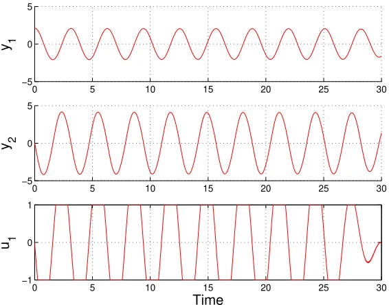
2.3.1. State and Control vs. Time. GenSim uses the results files to derive a continuous-time, continuous-state control rule. It then simulates the system with this rule to produce state and control time paths starting from a given initial condition. The performance index is also returned.

A very fine simulation step is necessary to yield smooth time paths from this problem’s control rule - here 75000 steps were used. Examination of Gaitsgory and Rossamakhine’s optimal time paths (see Figure 5 of [2]) suggests (2.1,0.1) as an approximate initial condition. Consequently,

GenSimwas called as:

GenSim(‘output’, [2.1, 0.1], 30*ones(1, 75000)/75000)

decreases with the time step: the transitions would have taken approximately 0.70 time units had half as many time divisions been used.

0 5 10 15 20 25 30

−5 0 5

y 1

0 5 10 15 20 25 30

−5 0 5

y 2

0 5 10 15 20 25 30

−1 0 1

u 1

Time

Figure 1. _{Approximated Time Paths.}

T can be estimated from Figure 1 as 3.14. The first and last peaks iny1 appear to occur at 3.15 and 28.23 respectively. This suggests calling GenSimagain as:

( GenSim(‘output’, [2.1, 0.1], 28.23*ones(1, 70575)/70575)

- GenSim(‘output’, [2.1, 0.1], 3.15*ones(1, 7875)/7875) )/25.08

yielding an estimate of ₋1.322 for the performance index, which closely agrees with Gaitsgory and Rossamakhine’s estimate of₋1.327 in [2]. The choice of TimeStepis important in deriving this value: halving the number of time divisions yields an estimate of only₋1.218.

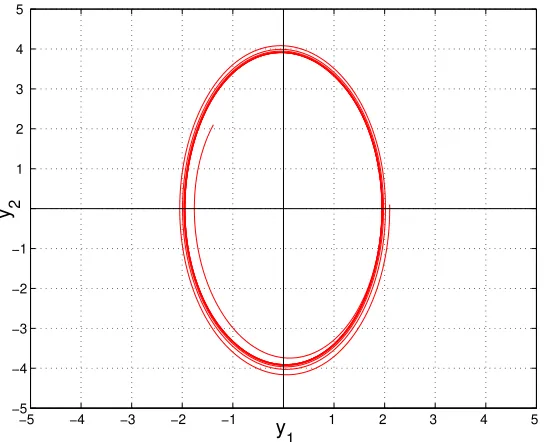
2.3.2. State vs. State. Plotting the pairs (y1, y2) from the time paths in Figure 1 yields the approximation of the optimal state trajectory shown in Figure 2. This corresponds closely to Gaitsgory and Rossamakhine’s approximation in Figure 1 of [2].

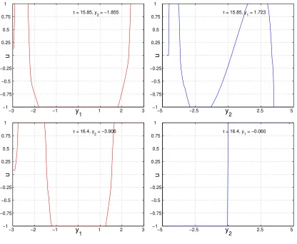
2.3.3. Control vs. State. ContRule graphs the control rule against the selected state variable for a specified time and value of the other state variable.

For a graph of the control rule againsty1 at (τ, y2) = (14.85,3.904), ContRule would be called as:

ContRule(‘output’, 14.85, [0, 3.904], 1);

−5 −4 −3 −2 −1 1 2 3 4 5 −5 −4 −3 −2 −1 1 2 3 4 5 y 1 y 2

Figure 2. _{Approximated Trajectory.}

Several similar calls were used to produce the control rules shown in Figures 3 and 4. The control rules are graphed against y1 (on the left) and against y2 (on the right) for four pairs (τ, y) taken from Figure 1.

−3 −2 −1 1 2 3

−1 −0.75 −0.5 −0.25 0.25 0.5 0.75 1 u y 1

τ = 14.85, y₂ = 3.904

−5 −2.5 2.5 5 −1 −0.75 −0.5 −0.25 0.25 0.5 0.75 1 u y₂

τ = 14.85, y₁ = 0.099

−3 −2 −1 1 2 3

−1 −0.75 −0.5 −0.25 0.25 0.5 0.75 1 u y 1 τ = 15.4, y

2 = 1.601

−5 −2.5 2.5 5 −1 −0.75 −0.5 −0.25 0.25 0.5 0.75 1 u y 2 τ = 15.4, y

1 = 1.778

As τ increases, a clear “flip” is evident in the control rules graphed against y1, reflecting the form of (6). Asy2 is out of phase with y1 by one quarter of a cycle, such a “flip” is absent in the control rules graphed againsty2.

−3 −2 −1 1 2 3

−1 −0.75 −0.5 −0.25 0.25 0.5 0.75 1 u y₁

τ = 15.85, y₂ = −1.855

−5 −2.5 2.5 5 −1 −0.75 −0.5 −0.25 0.25 0.5 0.75 1 u y₂

τ = 15.85, y₁ = 1.723

−3 −2 −1 1 2 3

−1 −0.75 −0.5 −0.25 0.25 0.5 0.75 1 u y₁

τ = 16.4, y₂ = −3.906

−5 −2.5 2.5 5 −1 −0.75 −0.5 −0.25 0.25 0.5 0.75 1 u y₂

τ = 16.4, y₁ = −0.060

Figure 4. _{More Control Rules.}

Note that Figure 2 of [2] is consistent with the upper-right plot in Figure 3, while Figure 3 of [2] is consistent with the lower-right plot in Figure 4.

2.4. System Specifications and Computation Time. The results presented here were de-rived in 2 days 9.32 hours on a computer having a 2.80Ghz PentiumR _{4 processor and 3Gb of}

memory. MATLABR _{version 7.2.0.232 (R2006a) with Optimization Toolbox version 3.0.4 was}

run on a Windows XP ProfessionalR _{operating system.}

As computation time rises linearly with the number of time divisions (see [3]), results could have been derived considerably faster by reducing the length of the time horizon to, say, 10.

References

[1] J.D. Azzato and J.B. Krawczyk.SOCSol4L: An improved MATLABR _{package for approximating the solution to}

a continuous-time stochastic optimal control problem. School of Economics and Finance, VUW, 2006. MPRA: 1179; available at: http://mpra.ub.uni-muenchen.de/1179/ on 14/02/2007.

[2] V. Gaitsgory and S. Rossamakhine. Linear programming approach to deterministic long run average problems of optimal control.SIAM J. Control Optim., 44:2006–2037, 2006.