Random WayPoint Mobility Model based Performance Estimation of MANET in terms of Average End to End Delay, Jitter and Throughput for CBR Application

Random WayPoint Mobility Model based Performance

Estimation of MANET in terms of Average End to End

Delay, Jitter and Throughput for CBR Application

M. K. Pandey

Amrapali institute of Management & Computer Applications

Uttarakhand Technical University

Sonika Kandari

Research Scholor Uttarakhand Technical University

ABSTRACT

In this paper, we are configuring an Adhoc mode scenario using QualNet as a Simulation tool to study impact of Random Waypoint mobility on QoS issues in MANET like Average end-to-end delay, jitter and throughput by varying number of nodes within a subnet. Different sets of reading were taken for six cases with varying number of nodes from 7 to 100 using CBR traffic type. We found that Random WayPoint Mobility Model works well with MANETs of large number of nodes as well, as the highest throughput is recorded for sixth case with 100 number of nodes. We conclude that Random WayPoint model with CBR traffic gives maximum throughput.

General Terms

Mobility Model, Random Waypoint Model, Mobile Ad Hoc Network, Constant Bit Rate Application.

Keywords

MANET, mobility, Random WayPoint model, Ad hoc scenario, simulation, QualNet, CBR.

1.

INTRODUCTION

Random Waypoint [1] is widely used in Adhoc network based simulation. In this paper, we have implemented Random WayPoint in QualNet 5.0 with varying number of nodes from 7 to 100. In RWP, each node of the network chooses uniformly at random a destination Point (“WayPoint”) in a rectangular deployment region. A node moves to this destination with a velocity „v‟ chosen uniformly at random in the interval [vmin, vmax]. When it reaches the destination, it remains static for a predefined pause time tp and then starts moving again according to the same rule.

2.

RELATED WORK

In [2],[3] and [4], the Node spatial distribution property has been studied. In [5] the author presented the exact, closed form expression of RWP node spatial distribution in one-dimensional networks, and a close approximation of the distribution. In [6] authors present a framework for studying mobility properties based on partial differential equations. The stochastic process underlying RWP mobility is defined in [7]. It has been observed in [8][9][10][11] that the spatial distribution of nodes moving according to the RWP model is non-uniform. Although the initial node positioning is typically taken from a uniform random distribution, the mobility model changes the distribution during the simulation. Performance evaluation of MANET routing protocols using Random WayPoint Mobility [12][13] is done by simulations

3.

MOBILE AD HOC NETWORK

A mobile Ad Hoc Network (MANET) is a spontaneous, self-organising network lacking fixed infrastructure or administrative support, where each mobile node is self-configurable and battery powered and often acts as a router of network packets. Each node in a MANET serves as a host and/or router generating, consuming or forwarding information . The depletion of participating nodes‟ battery power in a routing path will shorten the network lifetime. Dynamic nature and mobility characteristic impose several challenges to MANET routing protocols working under different scenarios. Under energy constrained operations, it is ideal to optimize energy use for extending network lifetime. Node mobility and/or break down of node due to loss of energy are possible causes of Topology changes in MANET . Maintaining an optimized state of a routing path in a network is quite difficult because the power of energy of nodes depends on the size, model, property, and capacity of the underlying battery . Transmission, reception and overhearing activities lead to depletion of energy in Batteries continuously Depletion of energy in intermediate nodes may disrupt communication resulting in modification of the network topology

4.

MOBILITY MODELS

4.1

File Based Mobility Model

User must specify Waypoints for all nodes. It is helpful in determining the node movement pattern in advance. The node position file contains related information in the format:

<Node-Id> <time><position>

where Node-Id is the Node Identifier, Time means simulation time for which the position is specified. A sample of .nodes file is shown as:

1 0 (513.98436684759997, 927.45535997310003, 0.00000000000000) 0 0

2 0 (826.30580620720002, 714.50892800539998, 0.00000000000000) 0 0

3 0 (815.65848441080004, 970.04464636659998, 0.00000000000000) 0 0

4 0 (584.96651215659995, 700.31249920749997, 0.00000000000000) 0 0

5 0 (624.00669207659996, 1030.37946875750004, 0.00000000000000)0 0

6 0 (737.57812457089994, 583.19196162530000, 0.00000000000000) 0 0

random selection of destination, speed and direction with inclusion of pause times between changes in direction and/or speed. After being at a location for certain duration of time, mobile node chooses random destination and speed at pre-defined range and proceeds towards newly chosen destination with velocity chosen. On reaching destination, mobile node pauses for a fixed time period before restarting the same process again. Here, speed and pause time help in defining the mobility behavior of nodes. Low speed and long pause time result in stable network topology whereas high speed and short pause time leads to dynamic topology.

4.3

Group Mobility Model

Group Mobility Model [14] simulates the movement pattern of a group of nodes. The vector sum of group mobility vector and internal mobility vector determine the mobility of the node under group boundary in simulation area. Group based node placement policy is used with group mobility model.

5.

DESIGNING OF SCENARIO

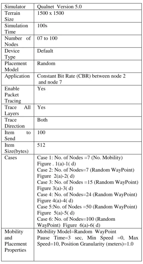
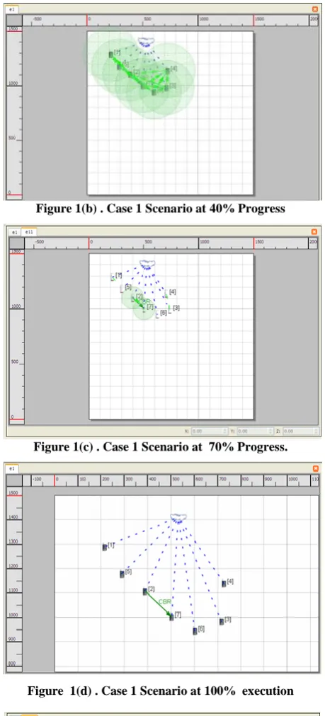
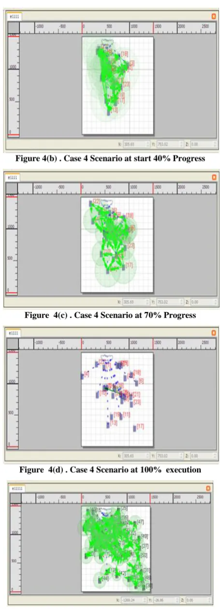
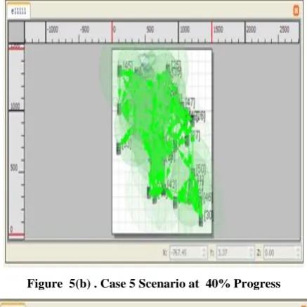
The scenario is designed initially with default device in the region of 1500 x 1500 with 7, 15, 24,50 and 100 nodes varying from no mobility (Case 1 with 7 nodes) to Random WayPoint mobility (Case 2 to Case 6, with 7,15,24,50 and 100 nodes) with wireless node connectivity keeping all nodes under one subnet. CBR application exists between node 2 and node 7 for all cases.

6.

PERFORMANCE METRICS

Average End-to-End Delay- is the delay of a packet in a MANET. The delay is the time the packet takes to reach the destination after it leaves the source. Jitter is the variance (difference) in end –to-end delay over time. It is measured in seconds. The amount of jitter that is tolerable is affected by the application type and the buffer size on the receiving side.

Throughput: is the average rate of successful bits delivered

to the sink, measured in bits per second. For any protocol, less average jitter gives better performance

7.

SCENARIO BASED SIMULATION

Our simulation study is comprising of the following phases: In first phase we have created and prepared the simulation scenario based on the cases as depicted in Table 1. In next step, we have executed, visualized and analyzed the created scenario and collected simulation results. Simulation results included scenario animations, runtime statistics, final statistics and output traces. Our last phase was to analyze the simulation results by configuring the parameters to collect the results and controlling the runtime performance.

Model

Application Constant Bit Rate (CBR) between node 2 and node 7

Enable Packet Tracing

Yes

Trace All Layers

Yes

Trace Direction

Both

Item to Send

100

Item Size(bytes)

512

Cases Case 1: No. of Nodes =7 (No. Mobility) Figure . 1(a)-1( d) Case 2: No. of Nodes=7 (Random WayPoint) Figure 2(a)-2( d) Case 3: No. of Nodes =15 (Random WayPoint) Figure 3(a)-3( d) Case 4: No. of Nodes=24 (Random WayPoint) Figure 4(a)-4( d) Case 5:No. of Nodes =50 (Random WayPoint) Figure 5(a)-5( d) Case 6: No. of Nodes=100 (Random

WayPoint) Figure 6(a)-6( d) Mobility

and Placement Properties

Mobility Model=Random WayPoint

Pause Time=3 sec, Min Speed =0, Max Speed=10, Position Granularity (meters)=1.0

Figure 1(b) . Case 1 Scenario at 40% Progress

Figure 1(c) . Case 1 Scenario at 70% Progress.

Figure 1(d) . Case 1 Scenario at 100% execution

Figure 2(b) . Case 2 Scenario at 40% Progress

Figure 2(c) . Case 2 Scenario at start 70% Progress

Figure 3(b) . Case 3 Scenario at start 40% Progress

Figure 3(c) . Case 3 Scenario at 70% Progress

Figure 3(d) . Case 3 Scenario at 100% execution

Figure 4(a) . Case4 Scenario at start of simulation

Figure 4(b) . Case 4 Scenario at start 40% Progress

Figure 4(c) . Case 4 Scenario at 70% Progress

Figure 4(d) . Case 4 Scenario at 100% execution

Figure 5(b) . Case 5 Scenario at 40% Progress

Figure 5(c) . Case 5 Scenario at 70% Progress

Figure 5(d) . Case 5 Scenario at 100% execution

Figure 6(a) . Case 6 Scenario at start of simulation

Figure 6(b) . Case 6 Scenario at 40% Progress

Figure 6(d) . Case 6 Scenario at 100% execution

8.

RESULTS AND DISCUSSIONS

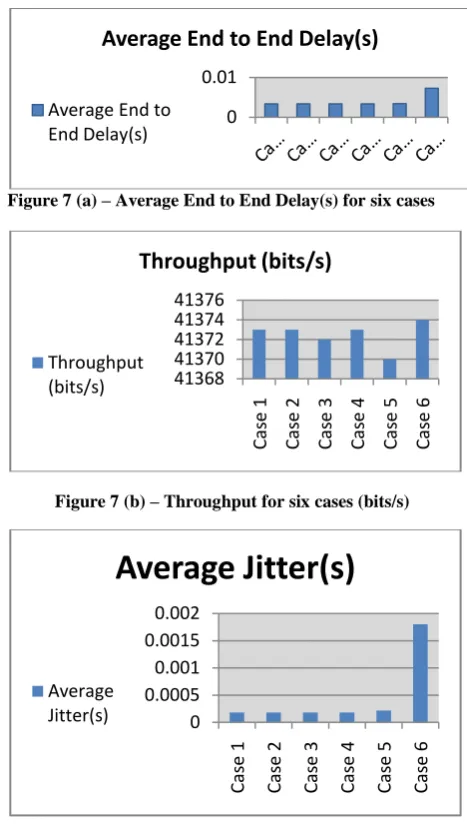
We have performed simulations for six different cases with varying number of MANET nodes ranging from 7 to 100 using Random WayPoint Mobility Model in QualNet Network Simulator. The results are summarized in in Table 2 and Fig 7 (a)- 7(c).

The comparison results show that by using Random WayPoint Mobility Model with varying scalability in MANET, the Average End to End Delay and Average Jitter values remains nearly same for slightly increasing the number of nodes but increases exponentially by doubling the nodes from 50 to 100 and will keep on increasing every time with multiple number of nodes (as is evident from value recorded for case 6). The reason behind this is the frequent link failures and consequently the overheads drawn to update all nodes with latest information. Highest throughput is recorded for sixth case with 100 (maximum) nodes along with high values of jitter and average end-to-end delay. This states that Random WayPoint Mobility Model is applicable for large sized MANETs.

Figure 7 (b) – Throughput for six cases (bits/s)

Figure 7 (c) – Average Jitter for six cases (bits)

Table 2 – Performance Metric for Simulation Result of six cases

Performance Metric Case 1 Case 2 Case 3 Case 4 Case 5 Case 6

Average End to

End Delay(s) 0.00337436 0.00337408 0.00337867 0.00339119 0.0034227 0.007291

Throughput (bits/s) 41373 41373 41372 41373 41370 41374

Average Jitter(s) 0.000179329 0.000179329 0.000181345 0.000182269 0.00021675 0.001801

9.

REFERENCES

[1] Bettstetter, C. and Wagner, C. 2002. The Spatial Node Distribution of the Random Waypoint Model. In Proceedings of First German Workshop Mobile Ad Hoc Networks.

[2] Bettstetter, C., Hartenstein,H. and Perez-Costa 2004. Stochastic Properties of the Random Waypoint Mobility Model. Wireless Networks. 10(5), 555-567.

[3] Bettstetter, C. and Krause, O. 2001. On Border Effects in Modeling and Simulation of Wireless Ad Hoc Networks. In Proceedings of IEEE Conf. on Mobile and Wireless Communication and Networks (MWCN).

[4] Blough, D.M , Resta, G. and Santi, P. 2004. A Statistical Analysis of the Long-Run Node Spatial Distribution in Mobile Ad Hoc Networks. Wireless Networks. 10, 555-567.

[5] Bettstetter, C. Resta, G. and Santi, P. 2003. The Node Distribution of the Random Waypoint Mobility Model for Wireless Ad Hoc Networks. IEEE Trans. On Mobile Computing. 2(3), 257-269.

[6] Garetto, M. and Leonardi, E. 2006. Analysis of Random Mobility Models with PDEs. In Proceedings of ACM MobiHoc, 73-84.

[7] Hyytia E., Lassila P. and Virtamo, J. 2006. Spatial Node Distribution of the Random Waypoint Mobility Model

[8] Bettstetter,C. 2001. Mobility Modeling in Wireless Networks: Categorization, Smooth Movement, and Border Effects. ACM Mobile Comp. and Comm. Review. 5(3)..

[9] Bettstetter, C. Resta, G. and Santi, P. 2002. A Statistical Analysis of the Long-Run Node Spatial Distribution in Mobile Ad Hoc Networks. In Proceedings of ACM Int‟l Workshop Modeling, Analysis, and Simulations of Wireless and Mobile Systems (MSWiM).

[10]Royer,E.M , Melliar-Smith, P.M and Moser, L.E. 2001. An Analysis of the Optimum Node Density for Ad Hoc Mobile Networks. In Proceedings of . IEEE International Conf. Comm. (ICC).

[11]Yoon, J., Liu, M. and Noble, B. 2003. Random Waypoint considered Harmful. In Proceedings of IEEE Infocom.

[12]Maurya, Ashish K, Singh, Dinesh and Kumar, Ajeet 2013. Performance Comparison of DSR, OLSR and FSR Routing Protocols in MANET Using Random Waypoint Mobility Model. International Journal of Information and Electronics Engineering 3(5), 440-443.

[13]Satya Sravani, B. , Prabhakar Rao, B. , Roopa Devi, B. 2014. Estimating the Performance Differentials of Different Protocols with varying Data Traffic. 3(7), 10827-10834.

[14]Hong, X., Gerla, M. , Pei, G. and Chiang, C.C. 1999. A Group Mobility Model for Ad Hoc Wireless Networks. In Proceeding of ACM International Workshop Modeling, Analysis, and Simulation of Wireless and Mobile Systems (MSWiM).

[15]Scalable Network Technology, QualNet 5.0 Simulator.Website:http://www.scalable-networks.com. [16]Corson S.,Macker J. 1999. Mobile ad hoc