Univariate Unobserved Component Model with Non Random Walk Permanent Component

Munich Personal RePEc Archive

Univariate Unobserved-Component

Model with Non-Random Walk

Permanent Component

Xu, Zhiwei

School of Economics, Shanghai University of Finance and Economics

11 November 2008

Online at

https://mpra.ub.uni-muenchen.de/12038/

Univariate Unobserved-Component Model with

Non-Random Walk Permanent Component

Zhiwei Xu

School of Economics, Shanghai University of Finance and Economics, Wuchuan Campus, Shanghai, 086-200433, China

[email protected]

December 9, 2008

Abstract

In this note, we revisit the univariate unobserved-component (UC) model of US GDP by relaxing the traditional random-walk assumption of the permanent component. Since our general UC model is unidenti…ed, we investigate the upper bound of the contribution of the transitory component, and …nd it is dominated by the permanent component.

Keywords: Unobserved-Component Model; Random Walk Assumption; Permanent and Tran-sitory Shocks

JEL classi…cation: C22; C49; E32

1

Introduction

Morley et al (2003) studied the equivalence of univariate unobserved-component (UC) model and the Beveridge-Nelson (BN) (1981) decomposition. They conclude that the permanent component of US GDP extracted by UC model is exactly the same as the BN trend. And the innovations of the two (permanent and transitory) components are highly negatively correlated (further discussions about this point can be found in a recent paper by Oh et al., 2008). The non-orthogonality of the two innovations is mainly caused by the random-walk

assumption imposed on the permanent component, as shown by Nagakura (2008). In this note, we relax the random-walk assumption by allowing the permanent component to follow a general unit root process. Under our assumption, the real GDP can be decomposed into two orthogonal parts so that impulse responses to permanent and transitory shocks can be generated. Since our generalization of the random-walk assumption increases the parameter set of the UC model, the model becomes unidenti…ed. However, we can investigate the upper bound of the contribution of the transitory component to GDP and study the dynamics of this extreme case by implementing impulse response and variance decomposition. We …nd that the transitory component explains less than 35% of total ‡uctuations in output, which is in sharp contrast to the existing literature.

2

The UC Model

Our modi…ed UC representation takes the form,

yt=gt+ct

gt= +gt 1+

q1(L)

p1(L)

t; si:i:d N(0; 2

) (1)

c_t= q2(L)

p2(L)

"_t; "_si:i:d N(0; 2 ")

where {yt} is log real GDP, {gt} is an unobserved permanent component with a unit root

(i.e., its …rst di¤erence is a ARMA(p1;q1) process with drift ). The unobserved

transi-tory component {ct} is a stationary ARMA(p2; q2) process. Moreover, we assume the two

innovations satisfy

cov( t; "t k) = f

" for k = 0

0 otherwise:

The parameters under interest include the mean growth rate ; and the coe¢cients of the two ARMA process,f p1(L); q1(L); p2(L); q2(L); ; "; "g:

Writing the model (1) more compactly gives the ARIMA representation of yt,

This expression implies we can recover the parameters of the UC model by estimating the growth rate of GDP as a ARIMA process. Here we follow the strategy of Morley, et al (2003)

to estimate GDP as an ARIMA(2,1,2) process1_:

(1 1L 2L 2

) yt = (1 1 2) + (1 + 1L+ 2L 2

)ut (3)

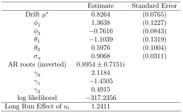
Table 1 reports the estimated results, note that j are the jth order autocovariance of MA

part of ARIMA process, and ; u and j are percentages. The data used is US quarterly

real GDP from 1948:I to 2008:I.

Table 1

Maximum Likelihood Estimates For ARIMA(2,1,2)

Estimate Standard Error Drift 0:8264 (0:0765)

1 1:3638 (0:1227) 2 0:7616 (0:0843) 1 1:1039 (0:1319) 2 0:5976 (0:1004) u 0:9068 (0:0311)

AR roots (inverted) 0:8954 0:7151i

0 2:1184

1 1:4505

2 0:4915

log likelihood 317:2356

Long Run E¤ect ofut 1:2411

The absence of real roots in AR part indicates that the polynomial (1 1L 2L 2

)

cannot be factored further. This fact induces us to determine the form of p1(L)and p2(L)

only in two alternative ways: p1(L) = 1; p2(L) = (1 1L 2L

2

)or p1(L) = p2(L) =

(1 1L 2L 2

).2 _{Obviously, the …rst case is just the speci…cation in Morley et al (2003) in}

which permanent component gt is a random walk. And the second case is the one we want

to discuss, in which gt is a general ARMA(2,2) process.

Once p1(L)and p2(L)have been determined, we can …nd the form of MA polynomials

q1(L); q2(L): In particular, to ensure the RHS of (2) be a MA(2) process, q1(L) and

1_{Oh et al (2008) also recommend this speci…cation. They …nd that ARIMA (2,1,2) is preferred by the}

AIC and ARIMA (1,1,0) is preferred by the BIC. But one shortcoming of the latter is that it cannot capture the periodical behavior of output due to its oversimpli…ed structure.

2_{The setting}

q2(L) can at most take the form of (1 + 1L+ 2L 2

)and (1 + L); respectively. Now the

parameters of interest are f 1; 2; ; ; "; "g3; and the representation (2) is reduced to

(1 1L 2L 2

) yt= (1 1 2) + 1 + 1L+ 2L 2

t+ (1 L) (1 + L)"t (4)

Remember that we have estimated the autocovariances of the RHS of last equation from the data, seef 0; 1; 2gin Table 1. Equate these moments to their counterparts in (4) and

after some algebra, we get three equations about f 1; 2; ; ; "; "g:

2

= 0+ 2 1+ 2 2 (1 + 1+ 2)

2

2 " =

2(1 + 1 1 2 )( 2 2 2

) ( 2)[ 0 (1 + 2 1+ 2 2) 2 ] 2 (1 + 1 1 2 ) 2( 2)(1 +

2

)

"=

[ 0 (1 + 2 1+

2 2)

2

] + 2(1 + 2

)( 2 2 2

) 2 (1 + 1 1 2 ) 2( 2)(1 +

2

) (5)

Since the MA(2) process has only three autovariances, we have six unknown parameters with just three equations. Therefore, this UC model is unidenti…ed.

In order to obtain two structural ( or orthogonal ) shocks, we need to set " to be

zero. The reader may ask whether this restriction is feasible4_{, since in Morley et al (2003),}

when permanent component is a random walk, two innovations are always highly negative correlated. In fact, as long as the long-run e¤ect (see the last row in Table 1) in the ARIMA representation of GDP is larger than 1, the orthogonality restriction in our modi…ed UC model is always feasible. A formal mathematical proof can be found in the Corollary 1 of Nagukara (2008).

To learn the relationships of the unknown parameters, one method is solve three of them as functions of the other two. Unfortunately, the system (5) is nonlinear and very complicated, we cannot solve it in a closed form. So we resort to numerical method. Figure 1 below plotsf 1; ; "gas functions of 2 when = 0:To conserve space, we do not report

cases when equals to other value in (-1,1), but the situations changes little. And to ensure

gt be invertible and 2

" always positive, 2 must be in the range about 0:6 to1.

3_{The mean growth rate is just the one in ARIMA representation.}

4_{Here, "feasible" means the equation system (5) always has solution when}

Figure 1 —The relationship between f 1; ; "g and 2 when = 0

One thing worth noting in Figure 1 is that f 1; ; "g are monotonic functions of 2,

and this feature does not change for di¤erent . Furthermore, the standard deviation of transitory shock "t reaches its maximum when 2 approaches to 1. Since " is a continuous

function of 2 and , without loss of generality, we …x 2 = 1 for di¤erent to …nd the

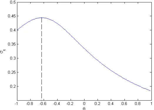
largest transitory component (in terms of variance) in our modi…ed UC model. Figure 2 plots " against , when 2 = 1.

Figure 2 — The maximum of " for di¤erent in (-1,1)

From the …gure, we can see " obtains its maximum of 0:4442 at = 0:63: In the next

parameter values (i.e., under the upper bound of the transitory component) and compare

the results with those obtained by using the Blanchard-Quah (1989) decomposition.

3

Dynamics

The largest possible variance of the transitory componentfctghas standard deviation0:4442

when setting = 0:63 and 2 = 1: The remaining parameters 1 and can be solved

directly from the equation system (5). In particular, we have 1 = 1:2612 and =

0:6059.5 _{Since both BQ (1989)}6 _{and our UC model implement orthogonal decomposition}

with a general unit-root permanent component, we can use impulse responses and variance decomposition to compare our results with theirs. To ensure consistency (i.e., GDP in the bivariate BQ decomposition must also follow a ARIMA(2,1,2) process), we estimate a 2-variable VAR system with GDP growth and unemployment rate as a vector ARMA(1,1)

process7_.

Figure 3 plots the impulse responses of GDP to a one-standard-deviation permanent and transitory shock respectively.8 _{In particular, under the permanent shock}

t( the left graph),

output in our UC model has a larger and periodic response compared with that obtained by the BQ method. The maximum response reaches its peak after six quarters. The long run e¤ect of the permanent shock is also signi…cantly larger (about 1.1), while under the

BQ decomposition this value is only about 0.6. Under the transitory shock "t (the right

graph);output movement in our model dies out quickly, while under the BQ decomposition the response is much larger and more persistent.

5_{The parameters {}

"; ; ₁} are statistically signi…cant, we calculate their t statistics by Monte Carlo

simulation, but not report here.

6_{In their paper, BQ decompose GDP based on a structural bivariate VAR system of ( GDP,}

Unemploy-ment rate). They just identify the model by imposing a long run restriction on transitory component. 7_{We implement this estimation by RATS 7.0 . One interesting thing is the VARMA(1,1) speci…cation}

reduces the estimation error greatly and all the parameters are highly signi…cant.

Figure 3—Impulse Responses of GDP to Di¤erent Shocks

a. Response to Permanent Shock b. Response to Transitory Shock

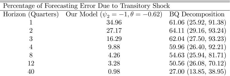
To see the relative importance of two shocks to the total variance of GDP, Table 2 reports the variance decomposition, i.e., the proportion of ‡uctuations due to transitory shock"t in

di¤erent forecasting horizons.

Table 2—Variance Decompositions in Di¤erent Models

Percentage of Forecasting Error Due to Transitory Shock

Horizon (Quarters) Our Model ( 2 = 1; = 0:62) BQ Decomposition

1 34.96 61.06 (25.92, 91.38) 2 27.17 64.11 (29.16, 93.24) 3 16.29 62.04 (27.50, 93.23) 4 9.88 59.96 (26.40, 92.21) 8 4.26 54.63 (25.94, 81.71) 12 3.28 50.56 (26.08, 70.12) 40 0.98 27.00 (13.85, 38.95)

The numbers in parentheses are 95% con…dence intervals. Even through these error bands of the BQ decomposition are large, contribution of transitory shocks to GDP are signi…cant lower in our model even compared with the lower bound of the BQ decomposition (except for the …rst period). That is, our model attributes most ‡uctuations of output to permanent shock; the transitory component is not important.

rate of GDP can be recovered as an ARMA(2,2) process. Table 3 below (in comparison

with Table 1) lists the implied parameters under the VARMA (asterisk indicates the value is signi…cantly di¤erent from the univariate ARMA(2,2) used in the UC model). Clearly, these di¤erent values implied by the VARMA (1,1) and the univariate ARMA (2,2) induce a much smaller long run e¤ect. This explains why the permanent shock in the BQ decomposition has smaller long run e¤ect than what we obtain in the UC model.9

Table 3—ARIMA(2,1,2) implied by VARMA(1,1)

AR Part MA Part Long Run E¤ect Log

1 2 1 2 of Innovation Likelihood

1:4863 0:5564 1:1969 0:2461 0:9149 0:7193 317:8866

4

Conclusions

This note has re-examined the UC method of decomposition of GDP by relaxing the random-walk assumption made in the existing literature. Based on this generalization, we are able to decompose GDP into two orthogonal components (permanent and transitory). This al-lows us to conduct impulse response analysis and variance decompositions. We …nd that the permanent component explains the bulk of GDP ‡uctuations, in sharp contrast to the conclusion reached by Blanchard and Quah (1989).

5

References

1. Beveridge,S., Nelson,C.R., 1981, A new approach to decomposition of economic time series into permanent and transitory components with particular attention to measure-ment of the business cycle. Journal of Monetary Economics 7, 151–174.

2. Blanchard,O.J., Quah,D., 1989. The dynamic e¤ects of demand and supply distur-bances. American Economic Review 79, 655–673.

3. Morley,J.C., Nelson,C.R., Zivot,E., 2003. Why are the Beveridge-Nelson and Unobserved-Components decompositions of GDP so di¤erent? Review of Economics and Statistics 85, 235–243.

9_{This point can be easily seen from a spectrum perspective: the spectrum of growth rate of GDP shares}

4. Nagakura,D., 2008. A note on the two assumptions of standard unobserved components models, Economics Letters 100, 123–125.