Performance Evaluation of First and Second Order Features for Steganalysis

Performance Evaluation of First and Second Order

Features for Steganalysis

Ashu

Student,M.Tech.(CSE)

Department of Computer Science and Engineering ITM University Gurgaon ,Haryana ,India

Rita Chhikara

Assistant Professor

Department of Computer Science and Engineering ITM University Gurgaon ,Haryana ,India

ABSTRACT

In this paper we have extracted various features from the images and evaluate their performance for various steganography tools with different classifier like J48, SMO, Naive bayes’s . There are so many steganography tools and many of them are changing the original images statistically during embedding process. To calculate that changes we are extracting various features from the cover image and stego image in spatial domain as well as DCT domain of JPEG image. Then train the classifier with the calculated feature vector of cover and stego image and evaluate features, that are more accurate to detect the hidden message. In this paper, we are using the three Steganography tools – nsf5 , PQ ,JPH&S with their different embedding efficiency like 10,25,50,100 percent .

Keywords

Steganography, Steganalysis, First Order Features , Second Order Features, Grey level Co-occurence Matrix, Global_block _hist.

1.

INTRODUCTION

Internet has become an important communication channel through which videos, images, emails, and speeches are easily transmitted and shared. For making secure communication over the internet there is the concept of cryptography and Steganography. Cryptography –secret writing. In this we encoded our message into another form in such a way that it can’t be understood by any third person. Steganography – cover writing. It hides the message so it cannot be seen by any third person[1].

Steganography is the art and science of hiding the presence of communication by embedding secret messages within any cover medium and that cover medium can be anything as digital images, videos, sound files [1,2]. A message is hidden information in the form of plaintext, cipher text, images or anything that can be embedded into a bit stream [2].A possible formula of the process represented as -

Cover medium+ Embedded message + Stegokey = Stego medium.

Steganography is also used by anti-social elements or criminals to hide their message within cover medium and make secure communication over the internet. So to detect the hidden message we need a technique .i.e. steganalysis. steganalysis is an art and science of detecting the hidden message from the cover medium .Steganalysis is used in computer forensics, cyber warfare, tracking the criminal activities over the internet and gathering evidence for investigations particularly in case of anti-social elements .The

objective of steganalysis is to collect sufficient information about the presence of embedded message and to break the security of its carrier. Thus steganalysis purpose is to defeat the purpose of Steganography. The goal of steganalysis is discovering the presence of hidden message and determining their attribute. In practice, a Steganography scheme is considered secure if no existing steganalytic attack can be used to distinguish between cover and stego objects [3].

1.1

Classification of Steganalysis

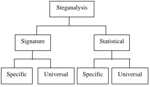
Fig. 1: Classification of Steganalysis

1.1.1. Signature Steganalysis

(on signature of the Steganography technique)Steganography methods hide secret information and manipulate the images and other digital media in such a ways that message is not detected by the human eye. But hiding information within any electronic media using Steganography methods requires alterations of the media properties that may introduce some form of degradation or unusual characteristics and patterns. These patterns and characteristics may act as signatures that broadcast the existence of embedded message.

1.1.2.

Statistical Steganalysis

In this technique statistics of an image is used to detect the secret embedded information .Specific/target steganalysis and universal/blind steganalysis are two major classes of steganalytic method.

Specific/target steganalysis – It include those statistical steganalysis techniques that target a specific Steganography embedding technique [3].

Steganalysis

Signature Statistical

Universal/blind steganalysis – not only for any specific embedding paradigm.it is applicable for any steganographic embedding algorithim.

Statistical steganalysis is better than the signature steganalysis because mathematical calculation gives better result than visual perception. Mostly steganalytic methods is based on the first order and second order statistics [3].

1.2

Different Steganalytic Method

There are serval trends appered in steganalysis.”chi –square attack ” by westfeld [4] was first general steganalyisis method. Firstly it was only for the sequentially embedded message and was later generalized to randomly embedded messages. but it is based on the first order statistics such as LSB(Least Significant Method). It has some disadvantge that its applicability to modern steganographic schemes is limited.

Another method of steganalysis is based on the concept of distinguishing statistics [5]. In this first carefully inspects the embedding algorithm then detect the length of the embedded message. It can be calculated by the detecting the changes in the cover images using calibration technique. Calibration was done in three steps: - first decompress the stego image, second crop the decompressed image by 4 pixel in each direction, third recompressed it again. But disadvantage of this approach is that detection needs to be customized to each embedding paradigm and it is difficult to design the proper distinguish statistics.

Third method is developed by blind classifier. Pioneered by Memon and farid [6]. In this method a classifier is trained to learn the difference between cover and stego image features. The 72 features are proposed by farid are calculated in the wavelet decomposition of the stego image. the biggest advantage of this method is that it is applicable to any embedded algorithm. But there was also some disadvantage i.e. this methodology will always be less accurate than targeted approaches and message length is also not accurately calculated.

So to solve this problem features is directly calculated from the DCT coefficients of JPEG images .In this method, a classifier is built using methods of artificial intelligent to distinguish in feature space between natural images and stego images[9,11].These features are based on the statistical properties of the JPEG DCT coefficients[8] .

2.

FEATURES BASED STEGANALYSIS

METHOD

2.1

Basic design of features based

Steganalysis

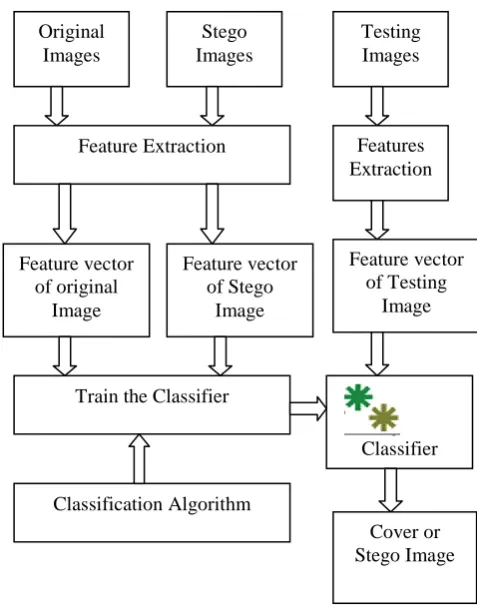
The main objective of the steganalysis is to detect the statistics changes in the cover image after hiding the message. For this there is a number of method and feature extraction is one of them . In 2005, Fridrich et al. introduced a method to detect stego images using first order features and second order features computed directly from the DCT domain since this is where most of the changes are made [7]. Then train our classifier on the various feature vector that is extracted from the cover images and stego images.

Fig :2 Block diagram of training and testing process for classification

2.2

Various features of Steganalysis

There are basically two type of statistics for calculating the features of images i.e. first order statistics and second order statistics The first order statistics calculate the intra block dependencies and it include the global histogram, individual histograms and dual histograms whereas, second order statistics calculate the inter-block dependencies, it include blockiness, co-occurrence matrix ,variation and markov feature .

2.1.1. First Order Features

In the first order statistic of DCT coefficients of JPEG images is their histogram like –

 global histogram

 individual histograms

 dual histograms

Suppose the stego images of JPEG file is represented with a matrix of DCT coefficient array d_k(i, j) where i, j = 1,…,8, k = 1, …, B. The symbol d_k(i, j) denotes the (i, j)-th DCT coefficient in the k-th block (there are total of B blocks)[10].

2.1.1.1. Global Histogram

In this calculate the histogram of all the 64k DCT coefficients.it is denoted as

H = (HL,...,HR),

(1)

Original Images

Stego Images

Testing Images

Feature Extraction Features

Extraction

Feature vector of original

Image

Feature vector of Stego

Image

Feature vector of Testing

Image

Train the Classifier

Classifier

Classification Algorithm

Where L = mini,j,kdi,j(k) and R = maxi,j,kdi,j(k). Central part of

this histogram is selected [-5,5] ,as maximam global histogram is situated there.

2.1.1.2. Individual Histogram

In this calculate the histogram of individual lower frequency DCT coefficients. It is denoted as

hi,j = (hLi,j ,... ,hRi,j) ,

(2)

where (i, j) ∈ {(1,2), (2,1), (3, 1),(2, 2), (1,3)} .

2.1.1.3. Dual Histogram

In this calculate the histogram of fixed coefficient value d, the dual histogram is an 8×8 matrix gdij.

𝑔𝑖𝑗𝑑 = B𝑘=1𝛿(𝑑, 𝑑𝑘 𝑖, 𝑗 ) , (3)

Where (i, j) ∈ {(2, 1), (3, 1), (4, 1), (1, 2), (2, 2), (3, 2), (1,3), (2, 3), (1, 4)}.

Where δ(u,v)=1 if u=v and 0 otherwise.

2.1.2. Second Order Features

When Steganography tools preserves the first order features then we calculate the inter block dependency based features i.e. second order features. It includes variation, Blockiness, co-occurence, markov features [8].

2.1.2.1. Variation

In this calculate the differences of coefficients in the same position in consecutive blocks first row-wise and then column-wise. The vectors of block indices are denoted as Ir,

while scanning the image by rows and Ic while scanning the

image by columns. It can be defined as

V=

𝑑_{𝐼𝑟 𝑘} 𝑖,𝑗 −𝑑_{𝐼𝑟 𝑘+1} 𝑖,𝑗 + 𝐼𝑟 −1

𝑘=1 8

𝑖,𝑗 =1 8𝑖,𝑗=1 𝑘=1 𝐼𝑐 −1 𝑑𝐼𝑐 𝑘 𝑖,𝑗 −𝑑𝐼𝑐 𝑘+1 𝑖,𝑗 |𝐼𝑟|+|𝐼𝑐|

(4)

2.1.2.2. Blockiness

In this calculate the difference between the pixel values at the boundaries of each JPEG block. The differences of the pixel values are calculated for both column and row boundaries and the sum of those gives our Blockiness value. Two Blockiness measures Ba are included in the functional for a =1,2 . .It can

be defined as

Ba =

|𝑔8𝑖,𝑗− 𝑔8𝑖+1,𝑗|𝑎 𝑁

𝑗 =1 [𝑀 −1_{8 ]}

𝑖=1 + 𝑀𝑖=1|𝑔𝑖,8𝑗− 𝑔𝑖,8𝑗 +1|𝑎 [𝑁−1_{8 ]}

𝑗 =1 𝑁 𝑀 −1₈ +𝑀[𝑁−1₈ ]

2.1.2.3. Co-occurence

In this calculate the probability distribution of neighboring JPEG coefficients. It is denoted as Cst .

𝐶𝑠𝑡 =

𝛿 𝑠, 𝑑𝐼𝑟 𝑘 𝑖, 𝑗 𝛿 𝑡, 𝑑𝐼𝑟 𝑘+1 𝑖, 𝑗 + 8

𝑖,𝑗 =1 𝐼𝑟 −1

𝑘=1 𝐼𝑐 −1𝑘=1 8𝑖,𝑗 =1𝛿 𝑠, 𝑑𝑐 𝑘 𝑖, 𝑗 𝛿 𝑡, 𝑑𝐼𝑐 𝑘+1 𝑖, 𝑗

Ir + Ic

(6)

2.1.2.4. Markov-Model Based features

In this markov model is used to detect the hidden message from the JPEG images.The difference between absolute values

of neighboring DCT coefficients is modeled as a Markov process. The quantized DCT coefficients F(u,v ), are arranged in the same way as the pixels in the image. The feature set is created by calculating four difference matrices from the quantized JPEG 2D array along horizontal, vertical, minor diagonal and major diagonal directions [9,10]. It can be defined as

𝐹ℎ 𝑢, 𝑣 = 𝐹 𝑢, 𝑣 − 𝐹(𝑢 + 1, 𝑣)

𝐹𝑣 𝑢, 𝑣 = 𝐹 𝑢, 𝑣 − 𝐹(𝑢, 𝑣 + 1)

𝐹𝑑 𝑢, 𝑣 = 𝐹 𝑢, 𝑣 − 𝐹(𝑢 + 1, 𝑣 + 1)

𝐹𝑚 𝑢, 𝑣 = 𝐹 𝑢 + 1, 𝑣 − 𝐹(𝑢, 𝑣 + 1)

(7)

Where, u ∈ [0,Su-2] , v ∈ [0,Sv-2] .Su is the size of the

quantized JPEG 2-D array in horizontal direction, Sv is the

size of array in vertical direction, Fh, Fv , Fd , Fm are the

difference arrays in horizontal, vertical, major and minor diagonals, respectively.From these four array, four transition probability matrices are constructed, namely, Mh , Mv , Md

,Mm as shows in equations

Mh 𝑖, 𝑗 =

𝛿(𝐹ℎ 𝑠𝑣 𝑣=1 𝑠𝑢−2

𝑢=1 𝑢, 𝑣 = 𝑖, 𝐹ℎ 𝑢 + 1, 𝑣 = 𝑗)

𝛿(𝐹ℎ 𝑢, 𝑣 = 𝑖) 𝑠_𝑣

𝑣=1 𝑠_{𝑢 −1} 𝑢=1

Mv 𝑖, 𝑗 = 𝛿(𝐹𝑣 𝑠𝑣−2 𝑣=1 𝑠𝑢

𝑢=1 𝑢, 𝑣 = 𝑖, 𝐹𝑣 𝑢, 𝑣 + 1 = 𝑗)

𝛿(𝐹𝑣 𝑢, 𝑣 = 𝑖) 𝑠𝑣−1

𝑣=1 𝑠𝑢 𝑢=1

Md 𝑖, 𝑗

= 𝛿(𝐹𝑑

𝑠𝑣−2 𝑣=1 𝑠𝑢−2

𝑢=1 𝑢, 𝑣 = 𝑖, 𝐹ℎ 𝑢 + 1, 𝑣 + 1 = 𝑗)

𝛿(𝐹𝑑 𝑢, 𝑣 = 𝑖) 𝑠𝑣−1

𝑣=1 𝑠𝑢 −1 𝑢=1

Mm 𝑖, 𝑗

= 𝛿(𝐹𝑚

𝑠𝑣−2 𝑣=1 𝑠𝑢−2

𝑢=1 𝑢 + 1, 𝑣 = 𝑖, 𝐹𝑚 𝑢, 𝑣 + 1 = 𝑗)

𝛿(𝐹𝑚 𝑢, 𝑣 = 𝑖) 𝑠𝑣−1

𝑣=1 𝑠𝑢 −1 𝑢=1

(8)

In order to reduce the computational complexity, they used a threshold value [-4, +4], i.e., any coefficient outside this range was converted to -4 or +4 depending on the value. This range will produce total of 81 x 4 = 324 features using the four difference matrices as probability transition matrix of 9 x 9 in each direction. To reduce the dimensionality, average the four probability transition matrices to get 81 features, i.e

M = (M(c) h +M(c)v +M(c)d +M(c)m )/4

(9)

3.

PROPOSED ALGORITHM

Using the concept of global histogram and grey level co-occurence matrix we proposed two algorithim for extracting the features of images one is Global_Block_hist and and another one is GLCM_Block.

3.1

Global_block_hist

INPUT

1. DIR – path of the directory of JPEG images. 2. N - size of block of Image.

OUTPUT

1. Feature – 11 feature of Image.

ALGORITHM –

Feature = GLOBAL_BLOCK_HIST(DIR,N)

2. Read the image and calculate the size of image. 3. Divide the image into the blocks of n rows and n

cols and get number of block rowwise( n_block_rows ) ,number of blocks colwise (n_block_cols).

4. Apply to all the blocks

a. Calculate the min value of each block hl.

b. Calculate the max value of each block. Hr.

c. Save the intensity value of block of image in between min and max value in variable h_o.

H_o = (hl,...,hr),

d. Normalize h_o by dividing each value of h_o with sum of h_o.

e. Store 11 centre values of h_o in vector f . 5. After step 4 , we get

F = n_block_rows *n_block_cols *11.

6. Calculate the mean of each 11 value with respect to all the blocks of image.

7. Save the 11 values calculated after mean , in final vector.

8. End.

3.2

GLCM_block

INPUT

1. DIR – path of the directory of JPEG images. 2. N - size of block of Image.

OUTPUT

1. Feature – 3 feature of Image. ALGORITHM –

Feature = GLCM_block (DIR, N)

1. Select the image from the dir of images one by one. 2. Read the image. And calculate the size of image. 3. Divide the image into the blocks of n rows and n

cols and get number of block row wise (n_block_rows), number of blocks column wise (n_block_cols).

4. Apply to all the blocks

a. Calculate the gray level co-occurrence matrix of block.

b. Normalize that gray level co-occurrence matrix of block.

 Transpose the glcm matrix.  Sumation of glcm and

transposed matrix.

 Divide the matrix by sumation of total number of elements.

c. Calculate contrast of normalize matrix (P) and save the value in final (1). It can be calculated as

𝑃𝑖,𝑗 (𝑖 − 𝑗)2 𝑁−1

𝑖,𝑗 =0

(10) d. Calculate energ of normalize matrix (P)

and save the value in final (2). It can be calculated as

𝑃𝑖,𝑗2 𝑁−1

𝑖,𝑗 =0

(11) e. Calculate homogeneity of normalize

matrix (P) and save the value in final (3).

It can be calculated as 𝑃𝑖,𝑗

1 + (𝑖 − 𝑗)2 𝑁−1

𝑖,𝑗 =0

(12) 5. After step 4,we get

Final = n_block_rows *n_block_cols *3.

6. Calculate the mean of each 3 value with respect to all the blocks of image.

7. Save the 3 values calculated after mean , in vector final.

8. End.

In this divid the extracted features into two category i.e. FBS (246) and FBS(95). FBS (246) consist of 165 first order features (11Global histogram, 55individual, 99 dual histogram) and 81 second order markov features. It is calculated from equation 1,2,3,8,9 .Whereas FBS (95) consist of 11 first order features (Global_Block_hist) and 84 second order features (81 markov ,3 GLCM_block_hist) .It is calculated from 2,8,9,10,11,12 .

4.

EXPERIMENT RESULTS

TABLE 1. ACR(accuracy rate) of features with different steganography tools using j48 classifier

J48

Algorithim

bpnz

FBS(246) FBS(95)

ACR ACR

NsF5

0.1 50.2 50.3

0.25 59.25 63.15

0.50 86.2 86.55

1.0 99.45 99.4

PQ

0.1 97.65 99.65

0.25 97.35 99.65

0.50 96.2 99.65

1.0 95.95 99.7

JPH&S 1.0 50.15 50

Table 2. Acr (Accuracy Rate) of Features with Different Steganography Tools using SMO Classifier

SMO

Algorithim

Bpnz

FBS(246) FBS(95)

ACR ACR

NsF5

0.1 50.65 51.5

0.25 85.7 79.5

0.50 98.35 96.65

1.0 99.9 99.95

PQ

0.1 99.95 100

0.25 99.9 100

0.50 99.9 99.95

1.0 99.9 99.95

JPH&S 1.0 57.15 48

TABLE 3. ACR(accuracy rate) of features with different steganography tools using Naive Baye’s classifier

Naïve Baye’s

Algorithim

Bpnz

FBS(246) FBS(95)

ACR ACR

NsF5

0.1 45.75 47.4

0.25 53 56.6

0.50 65.3 72.5

1.0 96.05 98.5

PQ

0.1 80.55 95.25

0.25 80.3 95.1

0.50 79.8 94.75

1.0 79.75 94.85

JPH&S 1.0 44.95 45

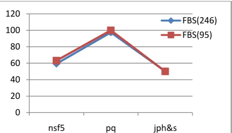
Fig3:Accuracy Rate for different Steganography methods for bpnz 0.25 using j48 classifier

Fig4: Accuracy Rate for different Steganography methods for bpnz 0.25 using SMO classifier

Fig5 : Accuracy Rate for different Steganography methods for bpnz 0.25 using

Naive Baye’s classifier

From this we analyse that features extracted from the FBS(95) is more accurate than FBS(246). In Naive Baye' it gives better result .

0 20 40 60 80 100 120

nsf5 pq jph&s

FBS(246) FBS(95)

0 20 40 60 80 100 120

nsf5 pq jph&s

FBS(246) FBS(95)

0 20 40 60 80 100

nsf5 pq jph&s

5.

SUMMARY AND CONCLUSION

Steganalysis is process by which we detect the secret information i.e. hidden by using the Steganography tool. Steganalysis is of two type –specific and universal steganalysis. Specific steganalysis is used for a specific Steganography algorithm whereas universal is used for any Steganography algorithm. There are various types of universal steganalysis and features based steganalysis is one of them. In this paper we use the features based steganalysis method to detect the hidden message.Three different steganographic methods, NsF5, JP Hide & Seek and PQ are used for hiding the secret information within images. We use four embedding rates: 0.10, 0.25, 0.50 and 1.00 bpnz. In the construction of the image database, 2300 images of same size (640 × 480). From the constructed database, 80 per cent is used for training and the remaining 20 per cent is used for testing. Then compare the performance of proposed features set with the state of art using three classification algorithm J48, SMO, Naïve Bayes in terms of accuracy rate. From the experiment result we conclude that FBS(95) gives better accuracy than FBS(246) . J48 and Naive bayes classifier gives us better result for FBS(95). We also conclude that in FBS(95) features vector length is also reduced as compare to FBS(246) so its execution time is also reduced.

6. REFERENCES

[1] J. Fridrich, M. Goljan, R. Du, Detecting LSB Steganography in color and gray-scale images, IEEE Multimedia Magaz., Special Issue on Security (October– November 2001) 22–28.

[2] N. Johnson, S. Jajodia, Exploring Steganography: Seeing the unseen, IEEE Comput. 31 (2) (1998) 26–34.

[3] Arooj Nissar , A.H. Mir : Classification of steganalysis techniques: A study

[4] Westfeld, A. and Pfitzmann, A.: Attacks on Steganographic Systems. In: Pfitzmann A. (eds.): 3rd International Workshop. Lecture Notes in Computer Science, Vol.1768. Springer-Verlag, Berlin Heidelberg New York (2000) 61−75

[5] Fridrich, J., Goljan, M., Hogea, D., and Soukal, D.: Quantitative Steganalysis: Estimating Secret Message Length. ACM Multimedia Systems Journal. Special issue on Multimedia Security, Vol. 9(3) (2003) 288–302

[6] Farid H. and Siwei, L.: Detecting Hidden Messages Using Higher-Order Statistics and Support Vector Machines. In: Petitcolas, F.A.P. (ed.): Information Hiding. 5

th

International Workshop. Lecture Notes in Computer Science, Vol. 2578. Springer-Verlag, Berlin Hei-delberg.NewYork(2002)340–354.

[7] J. Fridrich, “Feature-based steganalysis for JPEG images and its implications for future design of steganographic schemes,” in Information Hiding. Springer, 2004, pp. 67– 81.

[8] S. Lyu and H. Farid, “Detecting hidden messages use higher-order statistics and support vector machines,” in Information Hiding. Springer, pp. 340–354.

[9] Y. Shi, C. Chen, and W. Chen, “A Markov process based approach to effective attacking JPEG Steganography,” in Information Hiding. Springer, 2006, pp. 249–264. [10]Qingzhong Liu , Andrew H. Sung , Mengyu Qiao ,

Zhongxue Chen ,and Bernadette Ribeiro , “An improved approach to steganalysis of JPEG Images”