Numerical Analysis of Sensor Deployment in Wireless Sensor Network

Numerical Analysis of Sensor Deployment in Wireless

Sensor Network

Sudeep Shakya

Engineering

Kathmandu Engineering College Kalimati, Kathmandu, Nepal

Nirajan Koirala

Department of Electronics and Communication Engineering Kathmandu Engineering College

Kalimati, Kathmandu, Nepal

Narayan Nepal

Department of Electronics and Communication Engineering Research Coordinator, Office of

KEC Research and Publication (OKRP)

Kathmandu Engineering College Kathmandu, Nepal

ABSTRACT

Ad-hoc wireless network with a huge amount of static or mobile sensors is called wireless sensor network (WSN). The sensors collaborate to sense, collect and process the raw information of the phenomenon in sensing area (in-network), and transmit the processed information to the observers. Robustness, fault tolerance, and furthermore are prime factors to be consider before designing wireless sensor network. It is theoretically proved through math modeling, theoretical analysis and formula deducting that sensor deployments in the form of equilateral triangle, as a rule, are better than those in the form of square, hexagon and octagon. The theoretical analysis formula has given that minimum number of sensor nodes is demanded in a given sensor field if the field is covered fully and seamlessly and efficient coverage area ratio decrease with increase of sensor nodes comparing to same grid.

Keywords

Efficient coverage area; efficient coverage area ratio; sensor deployment grid; sensor nodes; sensor field; wireless sensor networks (WSN)

1.

INTRODUCTION

A wireless sensor network of devices to monitor physical or environment conditions. Due to their versatility, wireless sensor networks can be deployed to monitor conditions where using humans would either be too costly (in case of manpower and economy) or too dangerous. The versatility of these sensor networks lends them to a diverse variety of uses; from providing oceanographers information on areas previously unexplored to revolutionizing assisted living by ensuring loved ones can maintain their independence while still being unobtrusively monitored. The initial funding and research into wireless sensor networks was monitored by military needs to have autonomous battlefield surveillance [1, 2].

Wireless sensor networks are a quick growing area in research and commercial development. As research in sensor networks has grown, so too has the range of applications proposed to make use of this rich source of data. Coverage is the prime factor in wireless sensor network to maintain connectivity. Coverage in WSN is usually defined as a measure of how efficient and for how long the sensors are able to sense the sensor field [3]. As unique features, protocol design for sensor networks must account for the properties of ad hoc networks, including the following factors [3].

 Lifetime constraints imposed by the limited energy

supplies of the nodes in the network.

 Unreliable communication due to the wireless medium.

 Need for self-configuration, requiring little or no human intervention.

Connectivity can be defined as the ability of the sensor nodes to reach the data sink. If available route is not fixed in sensor node to the data sink then the processing of collected data by that node is not possible. Each node has a communication range which defines the area in which another node can be located in order to receive data. This is separate from the sensing range which defines the area that a node can sense. The two ranges may be equal but are often different. The rest of the paper is organized as follows: Section II introduces problem description where assumptions, definitions along with related works are explained. Sensor deployment has been explained in Section III. Efficient coverage area ratio based on different Sensor deployments like triangle, square, rhomb, hexagon and octagon are calculated in Section IV. Results and discussions have been described in Section V. This paper concludes with Section VI.

2.

PROBLEM

DESCRIPTION

2.1 Assumption

1. A sensors’ detecting ability is omnidirectional, that is, its coverage range is a disk whose radius r and whose area is D (D=πr2

).

2. In a sensor field, all sensors’ radio power is uniform, that is, the radio radius r of all sensors is equal.

3. In a sensor field, all sensors are in the same plane.

2.2 Definitions

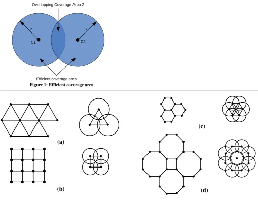
In the sensor field of wireless sensor networks, a piece of zone Z is possibly covered by several sensor nodes (Figure 1). In this case, the coverage resulted from Node C1 among these nodes is redundant for Zone Z. It’s because the information of Zone Z can be sensed and acquired by other nodes. Therefore, the definitions can be summarized as:

Definition 1: Efficient Coverage Area, : is the coverage area that is overlapping coverage zone Z’s area subtracted from node ’s coverage range (D=πr2), namely[3][5].

Definition 2: Efficient Coverage Area Ratio

2.3

Related Works

The analysis formula of the minimum number of nodes, the maximum efficient coverage area and its ratio, the maximum of net efficient coverage area of nodes and the maximum of net efficient coverage area ratio of nodes under the condition of seamless coverage. By analyzing both the deployments and considering different coverage redundancy requirement for different applications.

The paper analyzes several sensor deployments and computes their efficient coverage areas and their efficient coverage area ratios. In addition, the relation between the number of sensors and efficient coverage area ratio is discussed.

Figure 1: Efficient coverage area

3.

SENSOR

DEPLOYMENTS

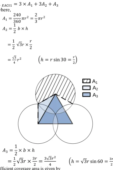
The sensor nodes are needs to be carefully placed exactly at the designated grid points. This method promises to provide certain percentage and degree of coverage and also the connectivity. Types of grids (Figure 2) used in networking; triangular lattice, square grids, hexagonal grids and one more grid is octagonal square grids [5-6].

3.1

Sensor Deployments Based on Square

3.1.1

Four sensors at four vertexes of the square

(its edge length is equal to r)

As illustrated in Figure3, Four sensors are respectively deployed at four vertexes of the square the length of which edge is equal to the length of the radius R of circle. The efficient coverage area is

Figure 2: Types of grids (a) Triangular lattice (b) Square grid (c) Hexagonal grid (d) Octagonal square network

C1 C2

r _r

Overlapping Coverage Area Z

Efficient coverage area

(a)

(b)

(c)

where,

For, r=1,

Its efficient coverage area Ratio is

Figure 2: The figure for computing efficient coverage area for four sensors at vertexes of square (edge length is r)

3.1.2

A meeting point of four circles

As illustrated in Figure 4, four circles intersect at the point at which the two diagonals of the square intersect. Obviously, the length of its edge is equal to . The efficient coverage area

is

where,

For r=1, It’s efficient coverage area ratio is

Figure 3: The figure for computing efficient coverage area for square

3.2

Sensor Deployments Based on Equilateral

Triangle

3.2.1

Three sensors at three vertexes of the

equilateral triangle (its edge length is equal to

r)

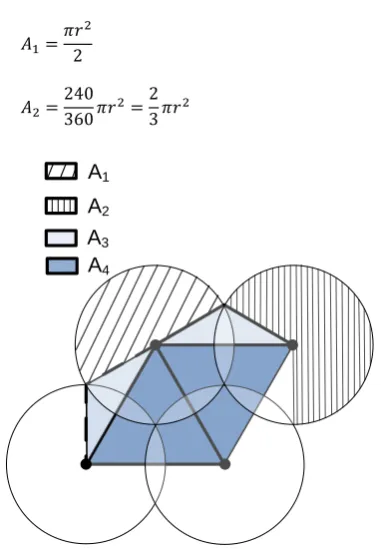
Three sensors at three vertexes of the equilateral triangle (its edge length is equal to r) as illustrated in Figure 5. The sensor deployment has the maximum efficient coverage area and the efficient coverage area is

where,

Efficient coverage area is given by

A

A

A

A1

A2

Figure 4: The figure for computing efficient coverage area for equilateral triangle.

For r=1,

Its efficient coverage area ratio is

3.2.2

Four sensors at four vertexes of the rhomb (its

edge length is equal to

r)

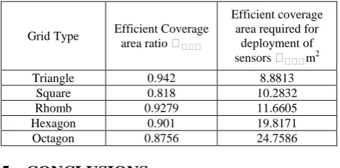
Four sensors are respectively deployed at four vertexes of the rhomb, the length of which edge is equal to r as illustrated in Figure 6 [8]. The efficient coverage area is

where,

Figure 5: Four sensor at four vertexes of the rhomb and computing effective coverage area

Efficient coverage area is given by

Its efficient coverage area ratio is

3.3

Sensor Deployments Based on Hexagon

The central circle intersects with six peripheral circles at six points which divide the central circle into six equal parts as illustrated in Figure 7. Obviously, the edge length of the hexagon is equal to radio radius r. The efficient coverage area of the sensor deployment is the area that the sum of the areas of seven circles subtracts the sum of the areas of 12 gray fields, that is, the efficient coverage area is

For b and h, we have

So,

For

The efficient coverage area

Figure 6: The figure for computing efficient coverage area for hexagon

A

A

A

A

A3 A1

For r=1,

Its efficient coverage area ratio is

3.4

Sensor Deployments Based on Octagon

The central circle intersects with eight peripheral circles at eight points which divides the central circle into eight parts as illustrated in Figure 8. The edge length of octagon is equal

For h, we have

For b and h

Figure 7: The figure for computing efficient coverage area for octagon

The efficient coverage area

Its efficient coverage area ratio is

4.

RESULTS

AND

DISCUSSIONS

The paper computed mathematically, simplifies coverage problem. In seamless WSN, it is theoretically proved node’s maximum efficient coverage area is A_EACt1=8.8813 and its maximum efficient coverage area ratio is R_ECAt1=0.942 for triangular grid, maximum efficient coverage area is A_EACr1=11.6605 and its maximum efficient coverage area ration isR_ECAr1=0.9279, maximum efficient coverage area is A_EACt1=10.283 and its maximum efficient coverage area ratio is R_ECAt1=0.818 for square grid, efficient coverage area is A_EACh1=19.8171 and its maximum efficient coverage area ratio is R_EACh1=0.901 for hexagonal grid and efficient coverage area is A_EACO1=24.75836 and its maximum efficient coverage area is R_EACO1=0.8756 for octagonal square grid. Triangular lattice is the best among the five kinds of grids as it has the smallest overlapping area hence this grid requires the least number of sensors, rhomb grid is best among rest of four grid, Octagonal grid and Hexagonal grid provide fairly good performance for any parameters while square grid is the worst among all since it has the biggest overlapping area (18.2% of total area coverage is overlapped). Other than type of grid the size of grid also play an important role.

Grid Type Efficient Coverage _{area ratio}

Efficient coverage area required for

deployment of sensors m2

Triangle 0.942 8.8813

Square 0.818 10.2832

Rhomb 0.9279 11.6605

Hexagon 0.901 19.8171

Octagon 0.8756 24.7586

5.

CONCLUSIONS

According to the listed table above, triangular lattice has the largest efficient coverage area ratio and uses least number of sensors compared to rest while square grid is worst as it has largest overlapping area. The earlier strategies commonly used to solve the WSN coverage problem considering only their benefits and costs. But, it can be concluded that by means of mathematical modeling, theoretical analysis and formula deduction, the effective coverage area ratio decreases with increase in number of sensor nodes comparing to same grid. In future we can calculate the effective coverage area ratio for any higher dimension lattice.

6.

Engineering College, Kalimati,Kathmandu,Nepal for the support and encouragement.

7.

REFERENCES

[1] Xueqing Wang, Fayi Sun, and Xiangsong Kong. “Research on Optimal Coverage Problem of Wireless Sensor Networks”. IEEE International Conference on Communication and Mobile Computing, 2009, pp. 548-551. [2] Xueqing Wang, Shuqin Zhang, “Research on Efficient Coverage Problem of Node in Wireless Sensor Networks”. IEEE Second International Symposium on Electronic Commerce and Security, 2009, pp. 532-536.

[3] Xingfa Shen, Jiming Chen, and Youxian Sun. Grid Scan, “A simple an Effective Approach for Coverage Issue in Wireless Sensor Networks”, IEEE International Communications Conference, June 2006 Volume:8, pp. 3480-3484.

[4] M. A. Perillo and W.B.Heinzelman, “Wireless Sensor Network Protocols,” University of Rochester., Rochester., NY, USA.

[5] Xueqing Wang, Yongtian Yang, Yibing Song. “ε-Redundant Movement-assisted Sensor Deployment Based on Virtual Rhomb Grid in Wireless Sensor Networks”, The proceedings of the 2006 IEEE International Conference on Mechatronics and Automation, 2006, 2006:pp. 775-779. [6] Vipin Saxena and Nimesh Mishra. (2013,March). UML

Modeling of Static Grid Octagonal Network Topology for Distributed Computing. volume (65-No.21), pages5-12. Available:

http://research.ijcaonline.org/volume65/number21/pxc3886 262.pdf

[7] Utkarsh Aeron and Hemant Kumar. (2013,March-April). Coverage Analysis of Various Wireless Sensor Network Deployment Strategies. Vol. 3-Iss2, pp. 955-961. Available: http://www.ijmer.com/papers/Vol3_Issue2/CG32955961.pd f