Commodity Price Volatility under New Market Orientations

(1)

Commodity Price Volatility under New

Market Orientations

Weaver, Robert D and Natcher, William C

Penn State University

2000

Online at

https://mpra.ub.uni-muenchen.de/9862/

(2)

Robert D. Weaver and William C. Natcher

Penn State University

Department of Agricultural Economics and Rural Sociology

March 2000

Paper Presented at the AES Annual Meeting 2000

Manchester, U.K.

(3)

Commodity Price Volatility under New Market Orientations

Robert D. Weaver and William C. Natcher*

*Professor and Research Assistant,

Department of Agricultural Economics, Pennsylvania State University

Abstract

Recent national and international regulatory reforms (e.g. U.S. FAIR and other GATT

compliance reforms) in agricultural markets has led some observers to wonder whether the

private sector is able to produce a level of price volatility that is socially acceptable. In this

paper, we examine the post reform track record of price volatility and its transmission across

vertically linked and geographically linked markets. Livestock, grain, and dairy market data

(monthly) are considered across the U.S. and E.C. The standard commodity-pricing model

supports the hypothesis that competitive storage acts to reduce the volatility of cash prices.

Further, speculative attacks and stock outs have been shown to induce increased volatility.

This motivates a scope of consideration that includes prices as well as stock levels to assess

their contribution to price volatility.

The paper considers evidence based on three decades of monthly data and advanced

time series techniques. First, univariate volatility estimates based on the autoregressive

conditional heteroskedasticity (GARCH) model are evaluated and compared to historical

temporal variation to highlight the importance of well grounded estimation of volatility.

Next, the relationships between stocks and the conditional mean, as well as the conditional

and unconditional variances of the price series, are assessed for dairy and grain products.

Finally, reform associated changes in the structure of the transmission of volatility through

vertical markets are considered for dairy products and across geographic markets is

(4)

Background.

Extensive literature over the past fifty years has considered the relationship between

inventory levels and price volatility. On the basis of such a relationship, a rationale for a role

for public sector management of commodity price volatility was developed showing that

governments could stabilize prices by managing stocks. However, the feasibility and

efficacy of such buffer schemes was later questioned when private sector intertemporal

arbitrage and government budget constraints were recognized, see Helmberger, et al. These

results were further strengthened as international trade and gaming among market

coordinating intermediaries (grain traders) were added to models. During the same period,

two other types of changes have influenced commodity markets: 1) expansion of the scope of

forward contracting mechanisms such as futures and options markets as well as the use of

forward contracting, and 2) liberalization of international trade. Over the past decades,

reforms in trade policy as well as government budget constraints has led to reduction of

government managed stocks. At the same time, private sector stocks have not expanded,

resulting in significant decreases in stock-to-use ratios for many commodities. These

changes in the government role in farm markets were most dramatically announced by the

F.A.I.R. Act in 1996. Extensive farm press and extension coverage (e.g. AgriFinance, 1997;

Yonkers and Dunn, 1996) has suggested that volatility would or has dramatically increased as

a result of F.A.I.R. However, the actual impacts of F.A.I.R. are unclear. First it was passed

after a substantial period of evolution in the role of government in farm markets. This is

highlighted in Figure 1 from which it is apparent that stocks-to-use ratios began to decline

sharply in 1986 to a new equilibrium level that was found in about 1989. From this

perspective, F.A.I.R. appears to have simply formalized an adjustment already accomplished.

(5)

volume. This setting motivates an examination of volatility in commodity prices over the

past several decades.

Of interest in this paper is the impact of changes in market conditions on the volatility

of commodity prices. Agricultural markets in the U.S. have been impacted by at least four

important types of policies that may have impacted price volatility: U.S. government farm

programs, and U.S. macro, trade and tax policy. The implications of each of these types of

policy for price volatility has received some attention in the literature. However, the joint

implications of changes in these policies has not been considered. Miranda and Helmberger

simulated the implications of government storage programs on competitive price stability

showing that it is feasible for public storage to stabilize market prices beyond the level

associated with perfectly competitive private storage. More broadly, the U.S. farm programs

have attempted to stabilize farm level prices through a combination of instruments and

actions including: setting of limit prices, price management through public storage and trade

transactions, subsidies for private on-farm storage, a variety of supply control instruments,

and trade policies. While a detailed modeling and simulation approach might be taken to

characterize and analyze each of the associated policy regimes, such an approach is

complicated by the jointness of the implementation of these programs as well as by

implementation that varied both temporally and spatially.

In very general terms, Crain and Lee identified three eras of post-World War II farm

programs: quota dominated, mandatory programs (January 1950- April 1964); acreage

control, voluntary programs (April 1964-December 1985); and increasingly market oriented

programs (December 1985 - 1997). Considering natural volatility of spot and futures wheat

prices across these programs Crain and Lee assumed volatility to constant across daily

observations within program regimes and found evidence that volatility had changed

(6)

was associated with each of the three regimes noted above. Crain and Lee conclude wheat

price volatility was higher in the 1964-85 policy regime then the 1985-93 regime. Using

dummy variables to characterize salient features of the policy regimes, they found that

mandatory and long-term land diversion programs are associated with low volatility in prices.

In contrast, they found low loan rates are associated with high levels of volatility. These

results provide support for press and extension observations concerning changes in volatility

that would be associated with F.A.I.R.

While these past studies are suggestive of a role of government programs in altering

the volatility of prices, the market setting for agricultural commodities is complicated

simultaneously by farm, tax, macro, and trade policies of both the U.S. and its trading

partners. Further, changes in government programs analyzed by Crain and Lee involved

numerous changes impacting incentives and constraints affecting private sector production,

storage, trade, and utilization decisions. The confluence of these policies and their

differential implementations suggest that a less structured approach to assessing changes in

price volatility is of interest. In this paper, we re-examine volatility within the most recent

of Crain and Lee regimes using less restrictive time series methods. We retain focus on the

particular regimes identified by Crain and Lee, however, we do so based on the interpretation

that the regimes reflect periods of common underlying political orientation toward

interventionist policy, rather than simple changes in farm policy.

Approach

To proceed, we evaluate volatility both over time and across commodities exposed to

different levels of policy intervention. We consider the past several decades of experience

for two commodities that have been the target of U.S. interventionist government programs:

wheat and corn. Further, we consider a substitute commodity, soybeans, which has not been

(7)

fundamentals as well as by competition for land. Finally, to allow for consideration of a

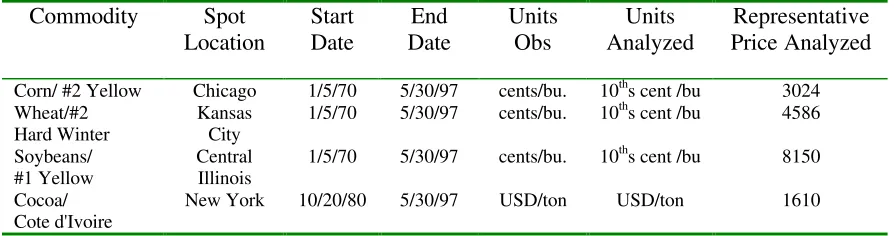
commodity that is much less influenced by U.S. policy, we consider cocoa. For each

commodity we analyze daily data to allow for consideration of volatility within trading

periods. Details on data are summarized in Table 1.

To analyze price volatility, define the price series as {Pt}. A natural estimator of the

volatility of prices has been based on measures of the variation within fixed marketing

intervals, see e.g. Poterba and Summers, Brunetti and Gilbert, Park, or Cho and Frees,

Peterson, et al.:

1)

∀ i=1,…I

where,

i=market interval

wi=interval width

ti=time of occurrence of the ith interval

The market interval has varied over studies, however, the utility of this measure relies upon

its consistency with the underlying data generating mechanism. Where the series {Pt} follows

a random walk in levels, and where the trading interval index i is set equal to the sampling

index (t) that indicates the observation date, then Si is estimated for each observation date and

1) provides an estimator of the conditional variance ht of {Pt}. Alternatively, where {Pt}

follows a random walk in logarithms of levels, 1) would not measure conditional variance.

In practice, trading interval width (wi) is defined based on market activity. In this study,

daily data is used and the trading interval is defined as the business week. Based on 1), the

market interval is allowed to vary to accommodate variation in the number of business days

in trading periods (e.g. due to holidays). To relate estimates of Si based on overlapping

intervals requires the additional assumption that prices generated within the interval (e.g. five

(

1

)

(8)

days of prices) follow from the same underlying distribution.

An alternative approach is to draw an estimate of conditional variance from a more

general model of the data generation process. Here, we allow for such a general form by

using a GARCH(1,1):

2)

∆Pt=β0 + β1∆Pt-1 + µt

where µt~N(0,ht) and ht=α0 + α1µ2t-1 + φ1ht-1 + νt. Furthermore, νt is assumed to be Gaussian.

By comparison to the natural estimator 1), an estimate of ht drawn from 2) provides an

estimate that varies over each observation without concern for specification of trading

intervals. In contrast, the natural volatility estimator provides only an estimate for each

trading interval, implicitly assuming the underlying stochastic process within that interval has

a constant variance. Further, the specification 2) allows for an autoregressive form in

differences, and an error that evolves according to a GARCH(1,1). When the observed price

series follows the process 2) with β0 = β1 = 0, the natural estimator provides a sample

estimate of ht for each observation. However, the small sample size within these market

intervals, and the likelihood that {Pt} does not follow a simple random walk, motivates a

strong interest in GARCH based estimates of conditional variance. To implement 2), we

impose the a priori restriction β0 = 0.

In order to identify the properties of the data generating process of Pt, we first

examine the characteristics of µt in equation 2) using Jarque-Bera test for normality as well as

direct tests of several alternative heteroscedastic forms. Results presented in Table 2 indicate

that the null hypothesis of normality is rejected for each commodity. The heteroscedasticity

tests were conducted to determine if the conditional variance of the series varies over the

(9)

approach (ARCH LM) to testing the hypothesis

Ho: c1=c2=...=cq=0

Ha: not Ho

as a restriction on:

3)

µ2

t=a + c1µ2t-1 + c2µ2t-2 + ... + cpµ2t-q + et

When the GARCH term is introduced, Lee (1991) shows the LM test for

GARCH(p,q) errors is identical to the LM test for ARCH(q) provided p≤q. In addition to

the ARCH LM test, two additional forms of heteroscedasticity were examined as noted in

Table (2). Each test regresses the squared residuals on a measure of the magnitude of the

dependent variable, the estimated price change and the squared estimated price change,

respectively. In both cases, these specific forms of heteroscedasticity are rejected. In

summary, the tests find strong evidence for non-normal residuals and motivates the use of a

GARCH specification.

In the financial literature, ARCH and GARCH processes have been extensively used

to estimate the conditional variance of price series and examine its evolution across a

changing economic environment, see Najand and Yung, Antoniou and Holmes, Baldauf and

Santoni. Baldauf and Santoni consider the impact of programmed trading on price volatility

by allowing the ARCH model of variance to change across two periods defined based on

existence of programmed trading. Antoniou and Holmes considered the impact of the

commencement of futures trading in the FTSE-100 Index on spot market volatility by

considering changes in an estimated GARCH process. Najand and Yung considered the

impact of changes in trading volume on the mean of a GARCH process.

GARCH and ARCH models have also been employed in the commodity market

(10)

Jansen, and Penson; and Chavas and Holt. Aradhyula and Holt applied a GARCH model to

retail meat prices to determine whether the conditional variances of the series varied over the

sample period. The results suggest the constant conditional variance assumption can be

rejected for the period and consequently the GARCH specification provided more

information about the precision of mean forecasts. Hans, et al. investigated the relationship

between the money supply and agricultural and industrial prices within a multivariate ARCH

and GARCH framework. Specifically, a vector autoregression (VAR) (G)ARCH model was

applied to the farm product price index, industrial product price index, and the money supply

(M1). The authors conclude the conditional mean and variance of agricultural prices are

more sensitive to changes in the money supply than are industrial prices. Moreover, the

results suggest the conditional mean and variance of the three variables exhibit a high degree

of correlation. Finally, Chavas and Holt evaluated the hog-corn price ratio and find evidence

that the process generating the pork cycle is nonlinear. Based on this finding the authors

apply a GARCH model to quarterly observations of the hog-corn price ratio and conclude the

model can account for some but not all of the nonlinearity.

The GARCH model provides a basis for interpretation of the nature of price

adjustment. Note the conditional variance from equation 2) can be written as,

(4)

ht=α0 + α1(µ2t-1 – ht-1) +(α1+φ1)ht-1 + νt

With this specification the term (µ2t-1 – ht-1) can be viewed as the shock to volatility while the

parameter α1 indicates the impact of recent innovations in price. Furthermore, φ1indicates

change in volatility induced by the accumulation of past innovations. Interpreting

innovations as news allows us to interpret these coefficients in terms of transient vs.

(11)

impacts of innovations.

Stationarity of a GARCH(p,q) process requires that,

(5)

Therefore, a GARCH(1,1) model is stationary if α1 + φ1<1. In the special case when the

parameters sum to unity, the GARCH model has a unit root and Engle and Bollerslev (1986)

refer to such a model as an IGARCH.1 That is, if (α1 + φ1)<1 then shocks will dissipate or

vanish while shocks will accumulate or persist if (α1 + φ1)≥1. The GARCH specification

provides a basis for examining market efficiency.represents a measure of efficiency. Under

an IGARCH process, shocks to volatility persist infinitely suggesting that arbitrage fails to

adjust the level of volatility to a long run equilibrium. Further, whenever φ1>0, finite

memory persistence exists suggesting markets are slow to react.

The issue of volatility persistence has been addressed by a number of authors in the

financial literature, e.g. Lock and Sayers, Poterba and Summers, and Chou. Locke and

Sayers investigate the relations between the arrival of information and the persistence of

volatility in the S&P 500 index futures market. The authors utilize a number of variables to

represent the flow of information such as contract volume, floor transactions, the number of

price changes, and executed order imbalance. They conclude that all of the variables explain

a significant portion of returns variance but even after information adjustment the S&P 500

returns continued to exhibit volatility persistence.

Another study which investigated the persistence of volatility in the equity markets

was conducted by Poterba and Summers (P-S). Here the authors examine the relationship

1

If the error term follows an IGARCH process, the unconditional variance of µt is infinite implying that any shock to the conditional variance has a permanent impact the unconditional variance. The unconditional variance of µt is expressed as,

σ2

=α0/(1-α1-φ1)

As the sum of α1 and φ1 tends to unity, σ2 tends to infinity and consequently, neither µt or µt2 satisfy the definition of covariance-stationary (Hamilton 1994). However, Nelson(1990) shows that σ2 is strictly stationary if α0>0 and the error term of the GARCH process is such that

∑ ∑

= =

< +

q

i

p

j j i

1 1

1

(12)

between price volatility and price levels for the S&P 500 index during the period 1928-1984

and the results suggest shocks to the market appear not to persist. Finally, Chou utilized a

GARCH model to investigate volatility persistence and changing risk premium in equity

markets and comes to an entirely different conclusion from P-S. That is, Chou finds a high

degree of volatility persistence in stock returns. He concludes the discrepancy between his

findings and P-S’s is the result data frequency. P-S utilized monthly observations while

Chou utilized weekly data.

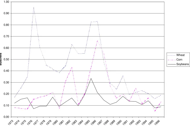
The price series analyzed are reported graphically in Figure 2. Several features of

price variation are apparent from these figures. First, substantial autocorrelation in direction

of change appears to exist for each of the commodities. Second, the variation of corn and

wheat appear to follow similar patterns and those patterns are distinct from those of soybeans

and cocoa. Stationarity of the underlying price series was examined using augmented

Dickey-Fuller tests and the results strongly support the conclusion that each price series is

I(1) in levels. This supports the interpretability of the natural volatility measure and motivates

the use of first differences in 2).

Natural volatility estimates based on a business week marketing interval are

presented graphically in Figure 3. Again, corn and wheat appear to follow similar processes

which are distinct from that followed by soybeans or cocoa. Further, the graphics suggest

that some autocorrelation in volatility exists. That is, high levels of volatility are followed by

subsequent periods of high volatility. This is strongest for corn and wheat, and weakest for

cocoa. A substantial shock to volatility is apparent for corn and wheat in late 1996, a period

associated with the introduction of the F.A.I.R. Act. The observed autocorrelation in

volatility further motivates the use of GARCH. Graphically, a further feature of importance

to note is that evidence of systematic increases in volatility are not apparent. This observation

(13)

was further supported by testing each volatility series for stationarity which resulted in the

hypothesis of unit root being rejected in every case.2 These findings of stationarity provide

evidence that supports the inference that a persistent data generating mechanism exists for

each price series over the sample period. Based on this inference, it is of interest to consider

the descriptive statistics that characterize these series. As noted in Table 1, the units for corn,

wheat, and soybeans are comparable, though their scales are not. As reported in Table 3, the

mean level of volatility for the sample period was 29.652 for corn, 26.214 for cotton, 41.222

for wheat, and 80.383 for soybeans suggesting that average volatility was highest for the crop

not managed by farm programs. Similar ordering of the commodities follows from a

comparison of the standard deviations of volatility – soybeans were found to have the highest

volatility. These results lend support to the conclusion of Miranda and Helmberger that

government storage programs can reduce price volatility. However, these results may be

misleading given that sample kurtosis and skewness values suggest each series is represented

by a non-normal distribution. Together the results further motivate the utility of GARCH.

Next, consider the GARCH results. The random walk hypothesis necessary for

interpretability of the natural estimates is rejected by the GARCH results. As is apparent

from Table 4, the coefficient of the lagged difference is statistically significant for each of the

commodities. This result implies that the use of natural volatility measures will be inefficient

(Mills ). ARCH and GARCH coefficients estimated in the GARCH(1,1) are statistically

significant and nonnegative with the exception of the GARCH coefficient for soybeans.

Results for the coefficient of the lagged innovation (α1 ) indicate comparable estimates in

2

The augmented Dickey-Fuller test was performed by estimating the following equation,

∆Pt= β1Pt-1 + β2∆Pt-1+…+βρ∆Pt-ρ + µt

(14)

magnitude for corn and wheat, both suggesting a small response to recent shocks. In

contrast, the results for soybeans indicate a more substantial response to recent shocks. The

GARCH coefficient φ1 indicates autocorrelation in conditional variance suggesting that some

persistence in volatility for corn, wheat, and cocoa (see Table 4). In fact, estimates are

consistent with IGARCH processes for corn and wheat. No significant persistence is found

for soybeans.

The unconditional variance estimates for each commodity during the entire sample

period and along within each regime is presented in Table 5. The unconditional variance has

also been normalized by the mean price change in each subperiod to allow for comparisons.

The results indicate corn and wheat are characterized by an IGARCH process during the first

regime while no such evidence is found during regimes 2 and 3. Alternatively. the

unconditional variance for soybeans and cocoa suggest a stationary GARCH process.

Comparing the normalized unconditional variance for each commodity indicates

soybeans experienced the highest level of volatility over the entire sample period. Notice that

the unconditional variance increased across regimes for both wheat and corn while

decreasing for soybeans and cocoa. Moreover, it appears that as public involvement was

reduced in the corn and wheat markets, price volatility became uniformly disbursed across

commodities.

The possibility of a systematic shift in volatility due to changes in market orientation

through changes in U.S. and trading partner farm, trade, macro, and tax policies can now be

investigated. First, we must recall that the estimated volatility series across the sample

appear to reflect no obvious structural breaks (see Figure 4). To proceed, we adopt three

policy regimes based on Crain and Lee's argument: acreage control, voluntary programs

(15)

-1993), and a period of substantial market reform (January 1994 – June 1997). While

structural breaks could be examined parametrically, in this paper, we limit our consideration

to these regimes.

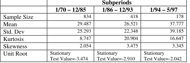
Two approaches are taken. First, the natural volatility series are reexamined within

these regimes. Tables 6a – 6d present descriptive statistics. Unit roots of the natural

volatility measures within regimes were rejected in each subperiod except for soybeans

during the period of January, 1994 to June, 1997. Although the volatility series appeared

stationary across the entire sample (1970-1997), the results in Tables 6a – 6d suggest that the

characteristics of volatility in each subperiod changed for each commodity. For example, the

mean level of volatility for cocoa decreased from 37.749 in the first period to 16.677 in the

final. Similarly, the standard deviation also decreased for cocoa in each period. That within

each regime except for the period 1/94 - 5/97 when the volatility of corn increased. A

common characteristic of all four commodities is that the mean level of volatility decreased

from the first period to the second period. And with the exception of cocoa the mean level

increased from the second to third periods.

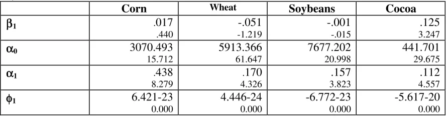
Next, the GARCH models were re-estimated within the policy regimes. Results

reported in Tables 7a – 7c provide the basis for several interesting inferences. First, it has

already been noted that policies impacting wheat and corn were progressively relaxed in a

definite movement toward stronger market orientation as regimes 1-3 are considered. As is

apparent from Table 7a – 7c, the persistence of volatility in corn and wheat decreases from

regime 1 through to regime 3 where no significant GARCH persistence is found. The

absence of persistence is found consistently across regimes for soybeans. These results

suggest that as market orientation in corn and wheat markets increased price volatility

became a contemporaneous phenomenon and persistence was not found. Furthermore,

(16)

identified with results supporting a random walk. In regime 2, a significant ARCH and

GARCH process is found with a strong persistence in volatility indicated. In regime 3, no

persistence is found, though a lagged impact of innovations is found.

Conclusion

The results from analyzing the prices of corn, wheat, soybeans, and cocoa for the

period January, 1970 – June, 1997 suggest a number of noteworthy characteristics. First,

price levels for each commodity appear to be I(1) while the volatility series is I(0). Next, the

natural volatility estimator suggests the level of volatility increased from 1970 to 1997 for

corn and wheat while the GARCH results suggest the persistence of volatility decreased. The

diminution of volatility persistence suggests these markets became increasingly efficient for

the period. Contrary to the corn and wheat markets, the mean level of volatility for soybeans

decreased over the sample period. Moreover for soybeans, no significant persistence was

(17)

0.00 0.10 0.20 0.30 0.40 0.50 0.60 0.70 0.80 0.90 1.00

1973 1974 1975 1976 1977 1978 1979 1980 1981 1982 1983 1984 1985 1986 1987 1988 1989 1990 1991 1992 1993 1994 1995 1996

Buschels

Wheat

Corn

[image:17.792.62.719.63.508.2]

(18)

Tables

Table 1. Heteroscedasticity Test Results3

Corn Wheat Soybeans Cocoa

Jarque-Bera* 744.98 14384.63 76741.60 1301.82

ARCH LM†

559.24 405.21 1058.48 167.17

ε2

t on y(hat)‡ .00 .00 .00 .00

ε2

t on y(hat)2 .30 1.43 .02 10.24

*5% critical value=5.99

†_{5% critical value=5.99}

[image:18.612.83.530.249.367.2]

‡_{5% critical value=3.84}

Table 2. Daily Price Data Analyzed

Commodity Spot Location Start Date End Date Units Obs Units Analyzed Representative Price Analyzed

Corn/ #2 Yellow Chicago 1/5/70 5/30/97 cents/bu. 10ths cent /bu 3024 Wheat/#2

Hard Winter

Kansas City

1/5/70 5/30/97 cents/bu. 10ths cent /bu 4586

Soybeans/ #1 Yellow

Central Illinois

1/5/70 5/30/97 cents/bu. 10ths cent /bu 8150

Cocoa/ Cote d'Ivoire

New York 10/20/80 5/30/97 USD/ton USD/ton 1610

Table 3. Distributional Statistics of Natural Volatility Estimates (Weekly)

Corn 1/70 - 5/97

Wheat 1/70 - 5/97

Soybeans 1/70 - 5/97

Cocoa 10/80 - 5/97

Sample Size 1430 1430 1430 867

Mean 29.652 41.222 80.383 26.214

Std. Dev. 26.832 38.046 93.712 18.870

Kurtosis 14.910 19.807 60.078 5.517

Skewness 3.056 3.199 5.952 1.982

Unit Root Unit Root

Test Value=-0.331 Unit Root Test Value=-0.068 Unit Root Test Value=-0.402 Unit Root

[image:18.612.84.547.406.582.2]

Test Value= -0.956

Table 4: GARCH(1,1) Summary Statistics

Corn Wheat Soybeans Cocoa

ββ1 0.022348

1.771 -0.023693 -2.005 0.085530 19.941 0.104694 6.473 3

1. Jarque-Bera: Test: (T-K)/6 [S2 + 1/4(K-3)2]~ χ22 where T= number of observations

K= kurtosis S= skewness

2. ε2t= β0+ β1ε2t-1 + β2ε2t-2

where the test statistic is: (T-2)R2~χ22 3. ε2t= β0+ β1y(hat)

where the test statistic is: TR2~χ21 4. ε2t= β0+ β1y(hat)2

(19)

α

α0 11.103924

12.992 5.871791 8.864 14745 43.873 3.667696 4.598 α

α1 0.122241

27.443 0.139187 28.599 0.367983 29.256 0.041037 15.977

φφ1 0.881215

[image:19.612.84.535.185.368.2]

251.696 0.878281 250.466 4.150461E-20 0.002 0.956916 382.394

Table 5. Unconditional Variance

Entire Sample

Unconditional Variance

-3,185.88 -336.15 23,330.10 1,791.74

Normalized -115.44 -9.09 312.76 75.90

Regime 1

-512.33 -266.68 31,553.90 2048.34

Normalized -18.66 -7.35 367.44 66.46

Regime 2

1,275.49 2,629.36 12,599.90 968.56

Normalized 50.89 82.16 217.81 43.83

Regime 3

5,463.51 7,124.54 9,107.00 497.41

Normalized 159.85 137.06 148.74 30.40

Table 6a. Subperiod Distributional Statistics of Natural Volatility Estimates (Weekly) for Corn.

Subperiods

1/70 – 12/85 1/86 – 12/93 1/94 – 5/97

Sample Size 834 418 178

Mean 29.487 26.521 37.777

Std. Dev 25.293 22.348 39.185

Kurtosis 8.747 20.904 16.647

Skewness 2.054 3.475 3.345

Unit Root Stationary

Test Value=-3.474

Stationary Test Value=-2.910

[image:19.612.84.443.402.522.2]

(20)

[image:20.612.82.445.93.218.2]

Table 6b. Subperiod Distributional Statistics of Natural Volatility Estimates (Weekly) for Cocoa.

Subperiods

10/80 – 12/85 1/86 – 12/93 1/94 – 5/97

Mean 37.749 22.985 16.677

Std. Dev. 22.862 15.421 8.733

Kurtosis 5.754 8.422 4.220

Skewness 1.503 1.896 1.144

Unit Root Stationary*

Test Value=-6.054

Stationary Test Value-5.107

[image:20.612.84.445.254.377.2]

*5% critical value is –1.95

Table 6c. Subperiod Distributional Statistics of Natural Volatility Estimates (Weekly) for Wheat.

Subperiods

1/70 – 12/85 1/86 – 12/93 1/94 – 5/97

Mean 39.448 36.637 60.299

Std. Dev. 38.541 26.240 51.412

Kurtosis 12.949 7.626 28.541

Skewness 2.607 1.941 3.919

Test Value=-3.407

*5% critical value is –1.95

Table 6d. Subperiod Distributional Statistics of Natural Volatility Estimates (Weekly) for Soybeans.

Subperiods

1/70 – 12/85 1/86 – 12/93 1/94 – 5/97

Mean 94.087 60.373 63.163

Std. Dev. 112.081 55.916 47.804

Kurtosis 49.164 25.990 9.827

Skewness 5.394 3.869 2.250

Test Value=-3.844

Non-Stationary Test Value=-1.484

[image:20.612.82.440.421.546.2]

(21)

[image:21.612.87.529.98.213.2]

Table 7a. GARCH(1,1) Parameter Estimates for the Period January 5, 1970 – December 22, 1985

ββ1 .006

.343* -.006 -.385 .068 5.689 .065 2.167 α

α0 4.661

5.636 5.067 7.903 19311 30.218 2044.248 39.409 α

α1 .131

17.677 .151 23.403 .384 19.405 .002 .202

φφ1 .878

[image:21.612.87.527.263.380.2]

154.552 .868 195.066 .004 1.042 4.332-23 0.000 * T-statistics

Table 7b. GARCH(1,1) Parameter Estimates for the Period December 23, 1985 – December 30, 1993

ββ1 .042

1.623 -.067 -3.818 .119 7.359 .108 4.913 α

α0 161.987

10.979 57.846 7.014 8530.115 25.454 8.717 3.987 α

α1 .207

11.425 .113 12.596 .323 12.740 .052 8.824

φφ1 .666

27.483 .865 94.615 8.685-24 0.000 .939 134.200

Table 7c. GARCH(1,1) Parameter Estimates for the Period December 31, 1993 – June 2, 1997

Corn Wheat _Soybeans _Cocoa

ββ1 .017

.440 -.051 -1.219 -.001 -.015 .125 3.247 α

α0 3070.493

15.712 5913.366 61.647 7677.202 20.998 441.701 29.675 α

α1 .438

8.279 .170 4.326 .157 3.823 .112 4.557

φφ1 6.421-23

[image:21.612.84.529.425.543.2]

(22)

References

Agri Finance (1997). "1996 Farm Bill Increases Risk." p. 24

Antoniou, A., and P. Holmes (1995) “Futures Trading, Information and Spot Price Volatility:

Evidence for the FTSE-100 Stock Index Futures Contracts Using GARCH.” Journal

of Banking & Finance Vol. 19 pp. 117-129

Aradhyula, S.V. and M.T. Holt (1988) "GARCH Time-Series Models: An Application to

Retail Livestock Prices." Western Journal of Agricultural Economics Vol 13 No. 2

pp. 365-374

Baldauf, B. and G.J. Santoni, (1991) “Stock Price Volatility: Some Evidence from an ARCH

Model” The Journal of Futures Markets, Vol. 11, No.2, pp. 191-200

Brunetti, C. and C.L. Gilbert (1995) “Metal Price Volatility”, 1972-95, Resource Policy, Vol.

21 No.4 pp. 237-254

Chavas, J. and M.T. Holt (1991) "On Nonlinear Dynamics: The Case of the Pork Cycle."

American Journal of Agricultural Economics pp. 819-828

Cho D.C., and E.W. Frees, (1988) “Estimating the Volatility of Discrete Stock Prices” The

Journal of Finance, Vol. XLIII pp. 451-466

Chou, R.Y. (1988) “Volatility Persistence and Stock Valuations: Some Empirical Evidence

Using GARCH.” Journal of Applied Econometrics Vol 3 pp. 279-294

Crain, S.J. and J.H. Lee (1996) “Volatility in Wheat Spot and Futures Markets, 1950-1993:

Government Farm Programs, Seasonality, and Causality.” The Journal of Finance

Vol. LI pp.325-343

Engle, Robert F. and Tim Bollerslev (1986) “Modelling the Persistence of Conditional

Variances.” Econometric Reviews Vol 5 pp. 1-50

Hamilton, James D. (1994) Time Series Analysis. Princeton University Press, Princeton NJ

Han, D.B., D.W. Jansen, and J.B. Penson, (1990) "Variance of Agricultural Prices, Industrial

Prices, and Money." American Journal of Agricultural Economics pp. 1066-1073

Helmberger, P.G., R.D. Weaver, and K.T. Haygood (1982) “Rational Expectations and

Competitive Price and Storage.” American Journal of Agricultural Economics Vol.

64. No. 2 pp. 266-270

Lee, J.H.H. (1991) “A Lagrange Multiplier Test for GARCH Models.” Economic Letters, 37, pp265-271

Locke, P.R. and C.L. Sayers (1993) “Intra-Day Futures Price Volatility: Information Effects

(23)

Miranda, M.J. and P.G. Helmberger (1988) “ The Effects of Commodity Price Stabilization

Programs.” The American Economic Review Vol. 78 pp. 46-58

Najand, M. and K. Yung (1991) “A GARCH Examination of the Relationship Between

Volume and Price Variability in Futures Markets.” The Journal of Futures Markets

Vol. 11 No. 5 pp. 613-621

Nelson, Daniel B. (1990) “Stationarity and Persistence in the GARCH(1,1) Model.”

Econometric Theory Vol 6 pp.318-34

Park, H.Y. (1996) “Trading Mechanisms and Price Volatility: Spot Versus Futures.” The

Review of Economics and Statistics pp. 175-179

Peterson, R.L., C. K. Ma, and R.J. Ritchey (1992) “Dependence in Commodity Prices.” The

Journal of Futures Markets Vol. 12 pp. 429-446

Poterba, J.M. and L.H. Summers (1986) “The Persistence of Volatility and Stock Market

Fluctuations.” The American Economic Review Vol. 76 pp. 1142-1151

Stuart, K. and C.F. Runge (1996) “Agricultural Policy Reform in the United States: An

Unfinished Agenda.” The Review of Marketing and Agricultural Economics.

Yonkers, R. D. and J.W. Dunn. "Managing Price Risk in the Absence of Government

Support Programs." Farm Economics. Pennsylvania State University, November,