G-Lets: A New Signal Processing Algorithm
B. Rajathilagam
Assistant Professor Department of Information
Technology Amrita Vishwa Vidyapeetham, Coimbatore,
India
Murali Rangarajan
Associate Professor Department of Chemical Engineering and Materials
Science Amrita Vishwa Vidyapeetham, Coimbatore,
India
K.P Soman
Professor Center for Excellence in Computational Engineering
and Networking Amrita Vishwa Vidyapeetham, Coimbatore,
India
ABSTRACT
Different signal processing transforms provide us with unique decomposition capabilities. Instead of using specific transformation for every type of signal, we propose in this paper a novel way of signal processing using a group of transformations within the limits of Group theory. For different types of signal different transformation combinations can be chosen. It is found that it is possible to process a signal at multiresolution and extend it to perform edge detection, denoising, face recognition, etc by filtering the local features. For a finite signal there should be a natural existence of basis in it’s vector space. Without any approximation using Group theory it is seen that one can get close to this finite basis from different viewpoints. Dihedral groups have been demonstrated for this purpose.
General Terms
signal processing, algorithm, group theory.
Keywords
signal processing, transformation groups, group theory, multiresolution analysis.
1.
INTRODUCTION
A digital signal is finite-dimensional. Therefore, within the approximation of digitization, the signal exists in a vector space of finite basis. If it is possible to obtain this basis of the signal space, a signal processing algorithm may be developed wherein the signal is projected onto the basis of the signal space to obtain its individual pieces. Such an algorithm would provide a general framework for extracting various features of interest from the signal without loss of information, within the digitization approximation. This is the inspiration behind the development of G-lets. Group theory [2][3][4][5][6] provides the crucial piece of the puzzle, namely the dimension of the vector space where the signal exists. Group theory also shows the way for choosing any suitable transformation or set of transformations required for a particular application customized to capture specific characteristics.
Fourier transform was first developed for continuous signals and then approximated for digital signals. In Wavelets, choosing a mother wavelet as an approximation of the signal, it’s translates and dilates are the actual basis functions. Since translations cannot be finite, it is also an approximation. In G-lets, we provide the most natural signal decomposition algorithm for a digitized signal without any artificially introduced approximations using general transformation groups.
2.
BACKGROUND
Fourier series generate a representation for a signal in terms of sine and cosine functions, giving an infinite set of basis vectors for the signal. Here time and frequency information cannot be localized on specific parts of the signal. Generalized Fourier basis is formed by creating representation matrices of the transformations and calculating their trace, which are called the characters of the transform. Wavelets [8][9] create orthogonal subspaces using the transformations dilation and translation to capture different frequencies of the signal. Still, due to the edge effect produced by breaking frequencies into smaller and smaller pieces, in applications like face recognition they are unable to testify a good match.
Ridgelet transform [10][11] focuses on detecting lines in an image using Radon transform [12]. Curves are specially recognized in a signal by curvelets [13], which is a combination of wavelets and ridgelets. These two transforms are specialized forms of wavelets. There are also other specialized forms of wavelets like the contourlets [14], wedgelets [15], and grouplets [16]. In grouplets, the wavelet coefficients are grouped together based on the direction of their flow using multiscale association fields. Representation theory using rotations and reflections have been used by Lenz [17][18] for edge detection in images but they do not generalize the use of transformation groups to generate an
orthogonal basis. In a recent work by Lenz, octahedral
transformation group has been chosen to be suitable for a specific application, i.e., the 3-D image environment, and representations have been used to describe this environment by evaluating their correlation coefficients. Vale [19] shows how an orthonormal set of polynomials can be generated by the orbit of a vector using representation theory [20][21]. In this work, we focus on using all the transforms of a transformation group using transformations like rotations, reflections, dilations, translations and more through their irreducible representations producing a series of block diagonal matrices portraying the features of the signal from low to high frequencies progressively. Dihedral groups [22][23] have been chosen for the illustrations.
3.
GROUP THEORETICAL APPROACH
A group is an ordered pair (G,*), where G is a set and * is a binary operation on G satisfying the following axioms:
Closure : For all a,b
ε
G, the product a * b is also in G.Associativity : For all a,b,c
ε
G, (a*b)*c=a*(b*c).Inverse: For every element a ε G, there is an element a-1,
called the inverse of a, such that a*a-1 = a-1*a =e.
If the elements of the group are linear transformations, then it is called a transformation group [24]. A transformation group is a set G of transformations of a certain set which has the following two properties:
1. If two transformations f and g belong to G then their
composition f o g also belong to G.
2. Together with every transformation f the set G also
contains the inverse transformation f-1.
Any two transformations h ε G and g ε G such that g = f * h*f
-1
are said to be conjugate transformations. The conjugate set of transformations split the group G into disjoint sets. There is another way of partitioning a group into disjoint sets using cosets. A coset is a subgroup of the group G obtained by choosing a subgroup H of the group first and then choosing another element a ϵ G, operate ‘a’ on H defined by the group G. If a is operated on the left(or right), then it is a left(or right) coset aH. This method is used by wavelets, with the mother wavelet the chosen subgroup of the transformation group G. Fourier transform is defined for cyclic transformation groups, where each element is commutative with every other element and also called the abelian group.
Fourier transform [22][25][26] is also extended to non-abelian groups, where each transform is reduced to the trace of its matrix representation due to which it lags the functionality to localize frequencies in time. If the conjugate partitioning of a group is used then no approximation is needed. An abstract group is brought alive by choosing any basis in the vector space of the signal. The group itself contains the linear
transformations on this vector space. Conjugate
transformations in the group collect together the
corresponding invariant subspaces of the vector space by deriving the irreducible representations of each linear transformation. These irreducible representations form the new basis for the signal called the G-lets. G-lets are not a single transform, but a set of transformations related by the rules of Group theory.
3.1
Constructing G-Lets
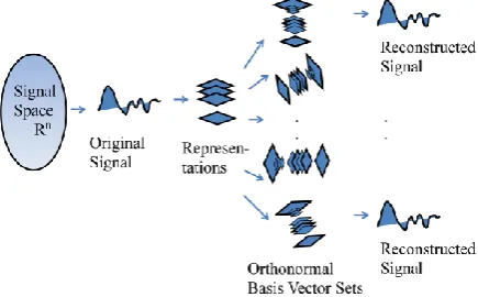
First a transformation group has to be chosen for generating G-lets. We focus only on finite groups whose representations are unitary so that they are always completely reducible into irreducible representations. A finite discrete signal is
considered. The signal exists in a vector space V, which shall
[image:2.595.59.277.612.747.2]henceforth be called as the signal space. For this signal, we generate a finite set of G-lets and project the signal on them. The signal can be reconstructed from G-lets without any loss as shown in Fig:1 below individually as well as through a linear sum of the transforms.
Fig 1: Representation matrices form a kaliedoscope
In the examples below the standard basis of the vector space V is the chosen basis of the signal given by
L = ni=1ei where ej = { 1 at i=j, 0 otherwise}
With this basis, the linear transformations materialize into matrices. The matrix representation looks like this:
D R =
D1 R 0
D2 R
D3 R
0 …
Each diagonal block Di(R) of the representation corresponds
to one irreducible representation. The procedure to find the irreducible representations is given below.
By Schur's orthogonality lemma, the irreducible
representations all put together are orthogonal and form a
basis for the vector space V.
Schur's orthogonality lemma 1: For finite dimensional representation of a finite group G in which inner products have been introduced to make the representations unitary
If R1 and R2 are two inequivalent irreducible
representations, then every matrix coefficient of R1
is orthogonal to every matrix coefficient of R2 with
respect to the inner product in the vector space V.
If R is another irreducible representations, then
G trace (R)
dim V is equal to the action of R on the other
irreducible representations R1, R2.
As a consequence, the dimensions of the irreducible representations follow the rule [2] [5]:
di2 m
i=1
= Dm
Where di = dimension of ith irreducible representation, Dm =
dimension of representation matrix and m = number of irreducible representations.
To show an example, we consider ‘Dihedral’ groups which include only two transformations, namely rotations and reflections. The conjugate transformations of the Dihedral groups occur either in pairs or remain single. Therefore the dimension of an irreducible representation is either one or two. If the dimension of the signal is ‘n’, then the basis is also of the same dimension. The representation matrix of the linear transformation is chosen to be of size n x n. The set of representation matrices for the transformations in the group
form what is called the representation space of dimension n2.
In a dihedral group Dn, there are ‘n’ rotations and ‘n’
reflections. Therefore there are 2n matrices one for each transformation. The rotation matrix is given by
Rθ = cos θ − sin θsin θ cos θ
0.766 0 0 0 0 0 0 0 0 0.766
-0.6428
0 0 0 0 0 0 0 0.6428 0.766 0 0 0 0 0 0 0 0 0 0.766
-0.6428
0 0 0 0
R1 =
0 0 0 0.6428 0.766 0 0 0 00 0 0 0 0 0.766 -0.6428
0 0 0 0 0 0 0 0.6428 0.766 0 0 0 0 0 0 0 0 0 0.766 -0.6428 0 0 0 0 0 0 0 0.6428 0.766
For dihedral groups, the number of irreducible representations is given by (n+6)/2 for even sized ‘n’ and (n+3)/2 for odd sized ‘n’. The matrix so formed is naturally a sparse representation. For other kinds of transformation groups, dimension of the corresponding irreducible representations are greater than two. Therefore the representation matrix can look like in the figure below with varying sizes of irreducible representations.
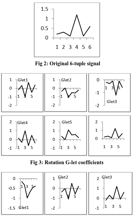
There are other transformation groups with combinations like rotations and translations, Heisenberg groups and etc. For illustration the G-lets for a 6-tuple sig = {0.2 0.3 0.1 1.2 0.1 0.6}is shown in the Fig:2, Fig:3 and Fig:4.
[image:3.595.317.541.69.153.2]Fig 2: Original 6-tuple signal
[image:3.595.53.289.69.203.2]Fig 3: Rotation G-let coefficients
Fig 4: Reflection G-let coefficients
[image:3.595.306.550.289.438.2]The figure above contains the original signal and both the G-lets corresponding to rotations and reflections respectively. More examples, of a 3-tuple and 9-tuple signal, with their G-let coefficients and representation matrices are shown in the appendix below. A comparison of G-let coefficients for a 9-tuple signal with Fourier and wavelet coefficients is shown in the following tables. Table 1 shows the G-let coefficients. Table 2 shows the Fourier and Wavelet coefficients for the same 9-tuple.
Table 1: Rotation G-let Coefficients
Rotation G-lets
Type G-let Coefficients
Signal -0.1259 0.3915 0.6 0.4454 -0.394 -0.7 -0.8 -0.6631 -0.194
G-let1 -0.0964 -0.0858 0.7113 0.5945 -0.0155 -0.022 -1.0628 -0.3833 -0.575
G-let2 -0.0219 -0.5229 0.4897 0.4654 0.3702 0.6663 -0.8283 0.0759 -0.687
G-let3 0.0629 -0.7154 0.039 0.1185 0.5827 1.0428 -0.2062 0.4996 -0.477
G-let4 0.1183 -0.5731 -0.4299 -0.2838 0.5226 0.9314 0.5123 0.6895 -0.045
G-let5 0.1183 -0.1627 -0.6977 -0.5533 0.2179 0.3842 0.9912 0.5568 0.4091
G-let6 0.063 0.3239 -0.639 -0.5639 -0.1887 -0.3428 1.0062 0.1635 0.6713
G-let7 -0.0219 0.6589 -0.2814 -0.3107 -0.5071 -0.9094 0.5504 -0.3062 0.6193
G-let8 -0.0964 0.6856 0.208 0.0879 -0.5881 -1.0505 -0.1629 -0.6327 0.2776
Table 2: Fourier and Wavelet Coefficients
Type Coefficients
Original Signal
0.1259 0.3915 0.6000 0.4454 -0.3940 -0.7000 -0.8000 -0.6631 -0.1940
Fourier -1.4401 1.2198 - 2.8035i -0.6931 + 0.2666i
-0.0007 + 0.3218i -0.3725 - 0.1655i -0.3725 + 0.1655i -0.0007 -0.3218i -0.6931- 0.2666i 1.2198 + 2.8035i
Wavelet 0.0049 0.3435 0.6646 -0.8694 -0.9594
-0.3011 -0.3168 0.2153 -0.1690 -0.1411 0.1836 -0.0997
4.
SALIENT FEATURES
Some of the salient features of this algorithm are discussed below:
It may be seen in Figure that the signal is portrayed by
representation matrices from different perspectives. The irreducible pieces might be big or small and that depends on the size of the signal. When a signal shows an irreducible representation of a large block size, it is possible to create an equivalent representation through a linear transformation with the help of its subspaces (null space or range space) such that the block becomes further reducible. This technique allows us to focus and explore further that part of the signal captured by the
0 0.5 1 1.5
1 2 3 4 5 6
-2 -1 0 1
1 3 5 Glet1
-2 -1 0 1
1 3 5 Glet2
-2 -1 0
1 3 5
Glet3
-1 0 1 2
1 3 5 Glet4
-1 0 1 2
1 3 5 Glet5
0 1 2
1 3 5
-1.5 -1 -0.5 0
1 3 5
Glet1 -2
-1 0 1
1 3 5 Glet2
-1 0 1 2
1 3 5 Glet3
0 1 2
1 3 5 Glet4
-1 0 1 2
1 3 5 Glet5
-2 -1 0 1
[image:3.595.53.281.367.736.2] [image:3.595.314.544.473.595.2]irreducible block as shown in Figures. The features of the signal under consideration are found to be spread across conjugacy classes, i.e., here they are spread across two conjugacy classes.
Fig 5: Irreducible blocks forming representation matrix
The number of irreducible representations is equal to the
number of conjugacy classes. Irreducible representations form the orthonormal basis. Conjugacy classes represent the structural symmetries for the signal. So, whenever a change occurs in the signal at a particular point, the above relationship propagates this change across different conjugacy classes.
When a representation is chosen for a signal, the
different basis of the underlying vector space gives different representations as if viewing through a kaleidoscope. We get a powerful method for matching the features of two signals especially in applications like pattern matching and face recognition with such a variety of basis sets.
Expanding any function f(x) in terms of the basis
functions of irreducible representations requires that the representation group is obtained by applying to the function f(x) all the transformations. Then the function is linearly expressible in terms of the basis functions in the various irreducible representations. One may also choose one of the irreducible representation functions g(x) with its projection of the signal and generate a new set of basis functions which will include itself in the set of basis functions. This feature allows us to customize the representation for any signal.
As the size of the signal increases, the number of
conjugacy classes is almost 50% less. This promises a compression of the signal, though further attention is needed in this regard. The Table 3 shows the number of conjugacy classes for different tuples.
Table 3: Number of Conjugacy Classes
S.No
Tuple
Odd/Even
No. of conjugacy classes (c) (n)
1 10 Even 8
2 21 Odd 12
3 32 Even 19
4 51 Odd 27
5 100 Even 53
6 501 Odd 252
7 1000 Even 503
In determining irreducible representations, a set of
reducible representations may be divided into lower angle matrices and higher angle matrices. The lower angle matrices may then be explored using a completely
different transformation group to further extract more features from that part of the signal.
Group representation theory states that, new
representations can be generated by direct product or tensor product of any two representation groups. Then their irreducible representations also turn out to be a direct product or tensor product.
It is also possible to use complex representation matrices
so long as a suitable transformation group is chosen. This quality could lead to the discovery of a new set of features in a signal.
Local features: The local features of a signal can be
identified by looking at the gradient map of each G-let. The same can be applied to G-lets at the next level where the G-let at the first level becomes the input to the second level. At each level, smaller and smaller local features are obtained.
Complexity: The computational complexity depends on
the number of viewpoints that need to be explored, the choice of transformation group and size of the signal. The matrices obtained in all of the representations are sparse orthonormal block-diagonal matrices and this adds an advantage for large signal calculations. Only if all the angles are to be explored, do we need to compute all the representation matrices and their corresponding G-let coefficients. One member of every conjugacy class put together shows a complete and different view of the signal. The same can be achieved by the alternate members of the conjugacy classes. In this way, the number of G-lets required for reconstruction of the signal can be cut down to the number of conjugacy classes.
5.
CONCLUSION
In this paper, a different approach to signal processing with the choice of a group of transformations is proposed. The results are demonstrated using the dihedral groups with rotations and reflections. The results provide a method of multiresolution analysis without an approximation like a mother wavelet. G-lets for other transformation groups need to be explored with a unique combination and characteristics and their suitability to different applications. G-lets can also be extended to a continuous signal in the Hilbert Space.
6.
REFERENCES
[1] Rajathilagam, B., Murali Rangarajan, and Soman, K.P.,
2011 G-lets: Signal Processing Algorithm Using Transformation Groups, IEEE Trans. Imag. Proc.,
submitted
[2] Riley, K. F., Hobson, M. P., and Bence, S. J., 2002
Mathematical Methods for Physics and Engineering, Cambridge University Press.
[3] Knapp, A. W., 1996 Group Representations and
Harmonic Analysis, Part II, Amer. Math. Soc., 43, 537-549.
[4] Duzhin, S.V., and Chebotarevsky, B.D., 2004
Transformation Groups for Beginners, Student
Mathematical Library, 25.
[5] Hamermesh, M., 1989 Group Theory and Its Application
to Physical Problems, New York, Dover Publications.
[6] Mallat, S., 1998 A Wavelet Tour of Signal Processing,
[7] Fokas, A.S., 1997 A unified transform method for solving linear and certain nonlinear PDEs, Proc. R. Soc. London A., 453, 1411-1443.
[8] Daubechies, I., 1988 Orthonormal bases of compactly
supported wavelets, Comm. Pure Appl. Math., 41, 909-996, October.
[9] Daubechies, I., 1992 Ten Lectures on Wavelets, Society
for Industrial and Applied Mathematics.
[10]Candes, E.J., 1998 Ridgelets: theory and applications,
PhD thesis, Stanford University.
[11]Candes, E.J., and Donoho, D.L., 1999 Ridgelets: the
key to high dimensional intermittency?, Phil. Trans. R. Soc. London A, 357, 2495-2509.
[12]Matus, F., and Flusser, J., 1993 Image representations
via a finite Radon transform, IEEE Transactions on Pattern Analysis and Machine Intelligence, 15, 996-1006.
[13]Candes, E.J., and Donoho, D.L., 2000 Curvelets and
curvilinear integrals, J. Approx. Theory, 113, 59-90.
[14]Do, M. N., and Vetterli, M., 2003 Contourlets, Beyond
Wavelets, Stoeckler, J, Welland, G. V., Ed., Academic Press.
[15]Donoho, D.L., 1999 Wedgelets: nearly-minimax
estimation of edges, Ann. Statist, 27, 859-897.
[16]Mallat, S., 2009 Geometrical grouplets, Appl. Comp.
Harmonic Analysis, 26, 161-180.
[17]Lenz,R., 1990 Group Theoretical Methods in Image
Processing, Springer-Verlag New York, Inc.
[18]Lenz,R., and Latorre Carmona, P., 2009 Octahedral
transforms for 3-D image processing, IEEE Trans. Image Processing, 18, 2618-2628, August.
[19]Vale, R., and Waldron, S., 2008 Tight frames generated
by finite nonabelian groups, Numerical Algorithms, 48, 11-27, July.
[20]Starck, J.L., Elad, M., and Donoho, D., 2005 Image
decomposition via the combination of sparse
representation and a variational approach, IEEE Trans. Image Processing, 14, 1570-1582.
[21]Aharon, M., Elad, M., and Bruckstein, A.M., 2006 The
K-SVD: An algorithm for designing overcomplete dictionaries for sparse representation, IEEE Trans. Signal Processing, 54, 4311-4322, November.
[22]Viana, M., and Lakshminarayanan, V., 2010 Dihedral
Fourier analysis, Lecture Notes in Statistics, Springer, New York, NY.
[23]Dresselhaus, M. S., 2008 Group Theory, Springer.
[24]Hamermesh, M., 1965 Group theory and its applications
to physical problems, Addison Wesley Publishing Company, Inc.
[25]Assefa, D., Mansinha, L., Tiampo, K. F., Rasmussen, H.,
and Abdella, K., 2010 Local quaternion Fourier transform and color image texture analysis, Signal Processing, 90,1825-1835, June.
[26]Stankovic, R. S., Moraga, C., and Astola, J., 1999
Readings in Fourier Analysis on Finite Non-Abelian Groups, TICSP Series,Sharp5, September.
Appendix
G-lets for a 3-tuple signal using the group D3 is shown below:
Rotation G-lets
Type Coefficients
Signal 44 55 34
G-let1 -22 -56.9449 30.6314
G-let2 -22 1.9449 -64.6314
Reflection G-lets
Type Coefficients
Signal 44 55 34
G-let1 22 -56.9449 -30.6314
G-let2 22 1.9449 64.6314
-0.5 0 0
R1 = 0 -0.5 -0.866
0 0.866 -0.5
-0.5 0 0
R2 = 0 0.5 0.866
0 -0.866 -0.5
1 0 0
R3 = 0 1 0
0 0 1
0.5 0 0
R4 = 0 -0.5 -0.866
0 -0.866 0.5
0.5 0 0
R5 = 0 -0.5 0.866
0 0.866 0.5
-1 0 0
R6 = 0 1 0
0 0 -1
G-lets for a nine tuple signal using the group D9 is shown as in Fig. The signal is chosen as
sig = [ -0.1259 0.3915 0.6000 0.4454 -0.3940 -0.7000 -0.8000 -0.6631 -0.1940 ]
0.766 0 0 0 0 0 0 0 0
0 0.766 -0.6428 0 0 0 0 0 0
0 0.6428 0.766 0 0 0 0 0 0
0 0 0 0.766 -0.6428 0 0 0 0
R1=
0 0 0 0.6428 0.766 0 0 0
0 0 0 0 0 0.766 -0.6428 0 0
0 0 0 0 0 0.6428 0.766 0 0
0 0 0 0 0 0 0 0.766 -0.6428
0 0 0 0 0 0 0 0.6428 0.766
0.1736 0 0 0 0 0 0 0 0
0 0.1736
-0.9848 0 0 0 0 0 0
0 0.9848 0.1736 0 0 0 0 0 0
0 0 0 0.1736 0.9848 - 0 0 0 0
R2 = 0 0 0 0.9848 0.1736 0 0 0 0
0 0 0 0 0 0.1736 0.9848 - 0 0
0 0 0 0 0 0.9848 0.1736 0 0
0 0 0 0 0 0 0 0.1736 0.9848
-0 0 0 0 0 0 0 0.9848 0.1736
-0.5 0 0 0 0 0 0 0 0
0 -0.5 -0.866 0 0 0 0 0 0
0 0.866 -0.5 0 0 0 0 0 0
0 0 0 -0.5 -0.866 0 0 0 0
R3 = 0 0 0 0.866 -0.5 0 0 0 0
0 0 0 0 0 -0.5 -0.866 0 0
0 0 0 0 0 0.866 -0.5 0 0
0 0 0 0 0 0 0 -0.5 -0.866
0 0 0 0 0 0 0 0.866 -0.5
-0.9397 0 0 0 0 0 0 0 0
0
-0.9397 -0.342 0 0 0 0 0 0
0 0.342
-0.9397 0 0 0 0 0 0
0 0 0
-0.9397 -0.342 0 0 0 0
R4 = 0 0 0 0.342
-0.9397 0 0 0 0
0 0 0 0 0
-0.9397 -0.342 0 0
0 0 0 0 0 0.342
-0.9397 0 0
0 0 0 0 0 0 0
-0.9397 -0.342
0 0 0 0 0 0 0 0.342
-0.9397
-0.9397 0 0 0 0 0 0 0 0
0
-0.9397 0.342 0 0 0 0 0 0
0 -0.342
-0.9397 0 0 0 0 0 0
0 0 0
-0.9397 0.342 0 0 0 0
R5 = 0 0 0 -0.342
-0.9397 0 0 0 0
0 0 0 0 0
-0.9397 0.342 0 0
0 0 0 0 0 -0.342
-0.9397 0 0
0 0 0 0 0 0 0
-0.9397 0.342
0 0 0 0 0 0 0 -0.342
-0.9397
-0.5 0 0 0 0 0 0 0 0
0 -0.5 0.866 0 0 0 0 0 0
0 -0.866 -0.5 0 0 0 0 0 0
0 0 0 -0.5 0.866 0 0 0 0
R6 = 0 0 0 -0.866 -0.5 0 0 0 0
0 0 0 0 0 -0.5 0.866 0 0
0 0 0 0 0 -0.866 -0.5 0 0
0 0 0 0 0 0 0 -0.5 0.866
0 0 0 0 0 0 0 -0.866 -0.5
0.1736 0 0 0 0 0 0 0 0
0 0.1736 0.9848 0 0 0 0 0 0
0
-0.9848 0.1736 0 0 0 0 0 0
0 0 0 0.1736 0.9848 0 0 0 0
R7 = 0 0 0
-0.9848 0.1736 0 0 0 0
0 0 0 0 0 0.1736 0.9848 0 0
0 0 0 0 0
-0.9848 0.1736 0 0
0 0 0 0 0 0 0 0.1736 0.9848
0 0 0 0 0 0 0
-0.9848 0.1736
0.766 0 0 0 0 0 0 0 0
0 0.766 0.6428 0 0 0 0 0 0
0
-0.6428 0.766 0 0 0 0 0 0
0 0 0 0.766 0.6428 0 0 0 0
R8 = 0 0 0
-0.6428 0.766 0 0 0 0
0 0 0 0 0 0.766 0.6428 0 0
0 0 0 0 0
-0.6428 0.766 0 0
0 0 0 0 0 0 0 0.766 0.6428
0 0 0 0 0 0 0
-0.6428 0.766
Reflection G-lets
Type Coefficients
Signal -0.1259 0.3915 0.6 0.4454 -0.394 -0.7 -0.8 -0.6631 -0.194
G-let1 0.0964 -0.0858 0.7113 0.5945 -0.0155 0.022 -0.0628 0.3833 0.5748
G-let2 0.0219 -0.5229 -0.4897 0.4654 -0.3702 0.6663 0.8283 0.0759 0.6867
G-let3 -0.0629 -0.7154 -0.039 0.1185 -0.5827 1.0428 0.2062 0.4996 0.4773
G-let4 -0.1183 -0.5731 0.4299 -0.2838 -0.5226 0.9314 -0.5123 0.6895 0.0445
G-let5 -0.1183 -0.1627 0.6977 -0.5533 -0.2179 0.3842 -0.9912 0.5568 -0.4091
G-let6 -0.063 0.3239 0.639 -0.5639 0.1887 -0.3428 -1.0062 0.1635 -0.6713
G-let7 0.0219 0.6589 0.2814 -0.3107 0.5071 -0.9094 -0.5504 -0.3062 -0.6193
Another example for G-lets of an ECG signal is shown here. The signal is a 168-tuple.
Some of the g-lets for this signal are shown below. The 1st
g-let is given by
The 10th g-let is given by
The 50th g-let is given by
The 100th g-let is given by
The above are rotation g-lets. The reflection g-lets are also
shown here. The 170th g-let is given by
The 200th g-let is given by
The 300th g-let is given by
In the above figures we see that there are oscillations in the signal. This is due to the two dimensional irreducible representations. The oscillations originate at a specific point in the signal and spread across the signal. This feature helps us to identify low and high frequencies. Filters can also be designed using various transformation groups.
-200 0 200 400 600 800 1000
1 10 19 28 37 46 55 64 73 82 91
100 109 118 127 136 145 154 163
-200 0 200 400 600 800 1000
1 11 21 31 41 51 61 71 81 91
101 111 121 131 141 151 161
-200 0 200 400 600 800 1000 1200
1 11 21 31 41 51 61 71 81 91
101 111 121 131 141 151 161
-1200 -1000 -800 -600 -400 -200 0 200 400 600 800
1 11 21 31 41 51 61 71 81 91
101 111 121 131 141 151 161
-1200 -1000 -800 -600 -400 -200 0 200
1
11 21 31 41 51 61 71 81 91 101 111 121 131 141 151 161
-1000 -500 0 500 1000
1 11 21 31 41 51 61 71 81 91
101 111 121 131 141 151 161
-1200 -1000 -800 -600 -400 -200 0 200
1 11 21 31 41 51 61 71 81 91
101 111 121 131 141 151 161
-200 0 200 400 600 800 1000 1200
1 11 21 31 41 51 61 71 81 91