Using Count Data Models in Travel Cost Analysis with Aggregate Data

Munich Personal RePEc Archive

Using Count Data Models in Travel Cost

Analysis with Aggregate Data

Hellerstein, Daniel

Economic Research Service, USDA

1991

Online at

https://mpra.ub.uni-muenchen.de/25264/

Using

Count

Data

Models

in

Travel

Cost

_Analysis

with

_Aggregate

Data

Daniel M. Hellerstein

In order to control for censoring and the integer nature of trip demand, the use of count data models in travel cost analysis is attractive. Two such models, the Poisson and negative binomial, are discussed. Robust estimation techniques that loosen potentially stringent distributional assumptions are also reviewed. For illustrative purposes, several count data models are used to estimate a county-level travel cost model using permit data from the Boundary Waters Canoe Area.

Key words: Boundary Waters Canoe Area, count data, negative binomial, Poisson, travel cost.

Estimators of recreational demand models fre- quently use continuous functional forms, such as ordinary least squares (OLS) on log trans- formed variables (e.g., Ziemer, Musser, and Hill). However, the nature of trip demand in- troduces complicating factors. First, trips occur in nonnegative quantities. Failure to control for this censoring will lead to biased estimation. Second, because trips are available only in in- teger quantities, the usual demand models, which correlate marginal quantity with marginal price, may be inapplicable.

In light of these factors, a natural alternative is to use statistical models that explicitly rec- ognize the "count" nature of trip demand. Sev- eral recent papers (e.g., Shaw, Smith, Grogger and Carson, Creel and Loomis) have applied count models to the travel cost model. These works largely have focused on truncated data sets based on choice-based samples. In this study the focus is on the older problem where zero-de- manders are included. In particular, the appli- cation of several robust estimators of count models to aggregated data will be considered.

The Poisson distribution forms the foundation for the count models examined in this study. Al- though the Poisson is a convenient distribution

to work with, it imposes some stringent con- straints on the demand distribution. In particu- lar, the Poisson distribution assumes the vari- ance of trip demand is equal to the expected value of trip demand. To loosen these constraints, a generalization of the Poisson, the negative bi- nomial, is discussed. Robust estimation proce- dures, that permit further loosening of a priori assumptions are then reviewed. Permit data from the Boundary Waters Canoe Area are used to examine the effects of these count models on consumer surplus estimates and on coefficient variability.

Theory

In formulating a demand process that yields count data, one must consider that trips are not avail- able in continuous quantities. The integer nature of the data can be explicitly accounted for by modeling the observed number of trips taken (over a season) as the result of many discrete choices (say, one for each day of the season). Under this scenario, count data distributions, such as the Poisson, are an asymptotic outcome.'

Therefore, in estimating a count model, the analyst is implicitly estimating the "daily" prob- ability of the recreator choosing to visit. In- creasing the travel cost will reduce the proba- bility of a visit on any given day. Following Small Daniel M. Hellerstein is a natural resource economist with the Re-

sources and Technology Division, Economic Research Service, U.S. Department of Agriculture.

Portions of this research were supported by the U.S. Forest Ser- vice Rocky Mountain Forest and Range Experiment Station.

The views expressed here are not necessarily those of either the Forest Service or the Economic Research Service.

The author acknowledges Robert Meldelsohn, Michael Moore, George Peterson, and A. Colin Cameron for their advice and as- sistance.

'If the probability of taking a trip on any given day is small, constant and independent of earlier decisions, and if the number of days in a season is large, then the distribution of trips will approach a Poisson process.

Hellerstein _{Travel Cost Analysis 861}

and Rosen, integrating over these price changes yields a measure of the compensating variation. Extending these results to the repeated discrete choice context yields a consumer surplus mea- sure over an entire season (Hellerstein and Men- delsohn). The key result is that count data models, as the limit of a repeated discrete choice pro- cess, can be used much like continuous models. In particular, integrating under a continuous es- timator of predicted demand will yield a mea- sure of consumer surplus.

Given this background, we concentrate on es- timating the expected value of trip demand. Fur- thermore, as a result of repeated discrete choice, the number of observed trips will follow a Pois- son distribution. Formally, the expected value of demand is

E(Y) = f(P, Z; P),

where E(Y) is the expected number of trips taken per season, P, Z are explanatory variables in- cluding travel cost to site (P) and demand shift variables (Z), such as income and travel costs to substitute sites, and

p

The Poisson probability distribution of de- mand is

(1)

Prob(Y = n; n = 0, 1, 2, ...) = exp(-A)A"/n! with A = f(P, Z; p).

The Poisson is a single parameter distribution with expectation and variance both equal to A (Mood, Graybill, and Boes). Although n is a nonnegative integer, A must be a strictly posi- tive real number.

The Poisson model is solved by estimating P, say P*, in A* = A(P, Z; /3*). The estimated value of A, A*, is interpreted as the predicted expected value (and variance) of demand. The predicted expected value of consumer surplus, E(CS), is then computed via the usual integration:

(2) E(CS) = A(P, Z; 8P*)dP,

where Pobs is observed price, and Pm, is a choke price, possibly 00

This paper will focus on this measure of con- sumer surplus estimated using the predicted mean of demand. Criticisms of this approach in the continuous context (see Bockstael and Strand; or Adamowicz, Fletcher, Graham-Tomasi) stress the importance of considering the source of er- ror. However, if measurement error is small, and

if the measure of expected demand is unbiased, then this measure of consumer surplus will be a good approximation to the expected value of consumer _surplus.2

Extending the Poisson: The Negative Binomial

A drawback to the Poisson model is the implied assumption that E(Y) and &(Y) are equal. Fur- thermore, Poisson "regressions" allow no ran- dom component in the A estimator; the A = A(P, Z; /3*) relationship does not contain an error component.

The negative binomial count model is often used to relax this unlikely condition of perfect knowledge of the A estimator and to permit more flexible variance/mean relationships. Following Cameron and Trivedi, the negative binomial is derived as a compound Poisson distribution, where A is assumed to be distributed as a gamma random variable.3 Integrating over this distri- bution of A yields the two parameter negative binomial. Formally,

Prob(Y = n, n = 0, 1, .. .)

F(n + P) V b F(n + 1)F(,) ,+ + P ,+ with

2

E(Y) = L and &(Y) = L +

The variance to mean ratio of the negative bi- nomial is a decreasing function of v. As

v

In terms of the repeated discrete choice framework, the negative binomial admits that

2 _{The concern is that E(CS(Y)) may not equal the CS(E(Y)), where}

the latter is what the analyst computes. However,

d(x; 0, E)dPdF(E) = d*(x; P)dP with d* = E(Y). Therefore, as long as E(Y) is unbiased, then E(CS(Y)), the left-hand side of the above equation, will approach CS(E(Y)), the right-hand side. It must be stressed that d* is an unbiased estimate of the expected value of demand. In particular, d* is assumed to explicitly account for censoring. When this con- straint cannot be guaranteed, an alternative form for d* = E(Y) (such as suggested by Maddala, p. 158) should be used.

Amer. J. Agr. Econ.

the underlying daily probability of visiting may be randomly distributed. More concisely, each individual is assumed to draw a value for her daily probability at the beginning of the season. Knowledge of the random process generating these daily probabilities is not required, so long as the net result is a gamma distribution of A, conditional on the exogenous variables.

Estimation

In addition to their appealing statistical proper- ties, the Poisson and negative binomial have several useful empirical properties:

(a) The sum of W independent Poisson var- iates is also Poisson distributed, with parameter A, = WAiA. Thus, the distribution of visits from the aggregate of W individuals is prob(Y = n) = _{(e- A)(Aw)n/n!. This adding-up property fa-} cilitates the use of aggregate data, given knowl- edge of population size.

(b) If a constant term is included in the func- tion describing A, the sum (over all observa- tions) of observed demand will equal the sum of predicted demand.

(c) Zero values are admissible. These prop- erties also hold for the negative binomial, with A replaced by ~t.

To insure that A (or g in the negative bino- mial) is strictly positive, it is postulated that (3) _{A(P, Z; 3) = exp(/30 + P/P + z8Z).} These count data models are estimated via max- imum likelihood (ML) techniques. The Poisson is readily estimated using the Newton-Raphson technique. The negative binomial, especially its Hessian matrix, is more complicated and is usu- ally solved with a quasi-Newton method, such as the BHHH or the DFP algorithms (Judge et al.).

Maximum likelihood estimation assumes that the postulated distribution is indeed correct. This assumption may impose some stringent require- ments, such as the E(Y) = 2(Y) criteria of the Poisson. The distributional sensitivity of these models raises concerns about robustness. How badly will these models fail if the true proba- bility distribution deviates from the assumed distribution?

The consequences of these assumptions, and possible means of relaxing them, have been studied by a number of authors. For count data models, the work of Gourieroux, Montfort, and

Trognon is especially useful.4 They introduce the concept of pseudo- (PML) and quasi-gen- eralized pseudo (QGPML) maximum likelihood estimation. Basically, they show that if func- tions describing the true mean and true variance of the dependent variable (say, the number of trips) are known [say, equal to f(p, z; P) and g(p, z; 8, a), respectively]; then the Poisson and negative binomial will be consistent, regardless of the underlying distribution. Several interest- ing results are obtained at the empirical level:

(a) For the Poisson, the estimates of

p

_p

(b) For the negative binomial, the ML esti- mate of

_p

An Application to the Boundary Waters Canoe Area

1980 permit data from the Boundary Waters Canoe Area (BWCA) in northern Minnesota will be used to compare the various count models. Each permit contains the ZIP code of the group leader, which can be used to obtain distance-to- site information as well as socioeconomic vari- ables either at the zip code level or at the county level. Because no other information is available, especially information on number of prior trips, the permits must be aggregated. County-level aggregates are used for this analysis. Therefore, the dependent variable is number of trips per county.

A total of 27,433 overnight permits were ag- gregated into the 1,396 counties within 1,000 road miles of the BWCA.5 About half of these

4 Other works in this field include White, who offers a general discussion of the consequences of using an incorrect distribution function, and McCullagh and Nelder, who embed count models in the framework of generalized linear models. An interesting sum- mary of count models as weighted, iterative linear estimators is presented by Hall, Hausman, and Griliches.

5 _{All overnight visitors are required to obtain a permit. The entire}

Hellerstein Travel Cost Analysis 863

counties have zero visits. Travel cost was based on $0.076/mile (1980$) plus a time cost com- puted using one-third of the per capita wage rate multiplied by average group size (4.0); the re- sult was an average cost per mile of approxi- mately $0.20.

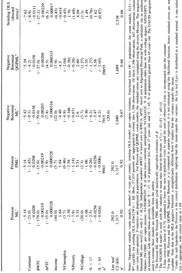
Table 1 contains the results from several models. An exponential form is used, with an individual's expected demand equal to exp(XPf), where X is a vector of exogenous variables. Be- cause aggregate data are used, the population of each county must also be considered. For the count models, the adding-up property suggests use of population as a multiplicative weight. Thus, _E(Y,,oun) = POP * _{exp(Xcon,,,,,);}

Y,,,ounis

the aggregate number of visits from the county, POP is the population of the county, and Xcounty

is a set of county-level exogenous variables (see table 1 for a description of the exogenous vari- ables). For comparative purposes, a simple per capita semilog model is also estimated. Con- sumer surplus (CS) estimates (in 1980$) are computed using equation (2), with equation (3) used for A*.6 _{In all models, the reported CS es-} timates use all 1,396 counties.

The most noticeable results are that the own- price coefficient (BWTC) is negative and sig- nificant for all models. This is especially true for the Poisson model. However, if the Poisson assumption of E(Y) = r2(Y) is incorrect, then the standard errors generated by the ML esti- mator of the Poisson will also be incorrect. To test this assumption, a score test devised by Lee is computed. This test is normally distributed under the null hypothesis that the Poisson model is correct. The results of this test, and the large value of the t-statistic for a in the negative bi- nomial model, indicate that the Poisson is in- appropriate [that E(Y) does not equal &2(Y)]. Thus, the CV matrix computed by the ML es- timator is incorrect, suggesting use of the PML estimator for the Poisson model. In the PML es- timator, BWTC is still significantly negative, but several of the demand shifters (the age vari- ables, percent unemployment, and percent pov- erty) are insignificant at the 95% level.

The negative binomial model returns quali- tatively similar coefficients for BWTC, % COL-

LEGE, and INCOME. The sign on the substitute price (APTC) is now positive, the theoretically anticipated sign. Also, the age variables are sig- nificant.

Within count models, the effect on consumer surplus is on the order of 25%. A much greater change (50%-100%) occurs between count and semilog OLS models. In RVD terms, given an average CS of $1.5 million, and a total of 25,000 groups of four individuals spending four days in the wilderness, the average RVD value will be about $4.00 (a fairly small value).

The semilog OLS model uses two heuristics: zero observations are dropped when coefficients are computed, and a bias correction factor is computed. The drop zeros rule ensures com- putability of the model. Since it discards infor- mation about nonvisitors, a potential for bias exists. Alternatively, the semilog model could be estimated using a nonlinear maximum like- lihood technique (Creel and Loomis). While such an approach permits zero visits, the treatment of demand shocks resulting from fluctuations in the error term (presumably caused by changes in unobservable factors) is not consistent with de- mand shocks caused by fluctuations in observed exogenous variables; with changes in unobserv- able factors having an additive impact, changes in observable variables have a proportional im- pact. Although this feature may or may not be appealing, for purposes of comparison the sim- pler drop zeros method is adopted.

The bias correction factor (Stynes, Peterson, and Rosenthal) is a simple multiplier guarantee- ing that the sum of observed demand equals the sum of predicted demand. It has substantial im- pact, leading to a doubling of CS. Alternatively, Bockstael and Strand argue against inclusion of such a bias correction factor. However, the bias correction factor is used since unbiased esti- mation of E(CS) requires an unbiased estimate of E(Y).

Formal qualitative comparisons between models are presented in table 2 and by exam- ining the 72 goodness-of-fit statistic in table 1.7 Table 2 displays the results of an out-of-sample test created by Ashley and popularized by Shaw.

6 To maintain consistency with the definition of the market area (all counties within 1,000 miles), a choke price equal to the max- imum price in the sample is used. Alternatively, a choke price of infinity could be used. However, when CS is computed using a choke price of infinity, the results differ by less than 1%. Note that the market area is limited in order to limit the bias resulting from visitors who partake in multiple-destination trips.

7 The 712 statistic can be described as a measure of the corre-

P E Oq rr c, \O \O c,

a a

a c5 O X

Table 1. Results of Count Models, 1980 BWCA Permit Data

Negative Negative Semilog OLS Poisson Poisson Binomial Binomial _(discard

MLa PMLa MLb _{QGPMLb zeros)c}

-5.14 -5.14 -5.42 -5.39 -7.62

Constant (-23.0) (-2.45) (-9.3) (-4.2) (-8.9)

-0.0208 -0.0208 -0.0158 -0.0158 -0.0111

BWTC (-179.0) (-15.0) (-79.0) (-27.0) (-27.2)

-0.00219 -0.00219 0.00203 0.00209 0.00229

APTC (-15.0) (-1.9) (7.4) (4.5) (6.5)

0.000328 0.000328 0.000316 0.000315 0.00017

Income (44.0) (5.7) (22.0) (7.9) (4.45)

1.64 1.64 -4.40 -4.5 -0.614

%Unemploy (3.7) (0.46) (-4.9) (-2.04) (-0.45)

-2.58 -2.58 -0.346 -0.381 1.70

%Poverty (-7.9) (-1.14) (-0.67) (-0.28) (1.69)

5.51 5.51 2.6 2.60 4.09

%College (20.0) (2.3) (3.7) (1.57) (3.3)

-1.06 -1.06 -5.46 -3.55 1.49

% < 17 (-2.5) (-0.26) (-4.2) (-1.27) (0.76)

-0.0256 -0.0256 -5.47 -5.58 1.62

% > 65 (-0.054) (-0.006) (-4.2) (-2.05) (0.87)

ad 9943 7915 29855

(20.0) Lee teste 292.0 292.0

CS (k$) 1,317 1,317 1,680 1,689 2,538

712 0.92 0.92 0.67 0.66 0.68

Notes: Dependent variable: count models, number of visits per county; semilog OLS model, per capita visitation. Functional form (W = population): for count models, E(Y) W* exp(XP); for semilog OLS, E(ln(Y/W)) = XP. Here, 27,433 permits are aggregated by county into 1,396 observations. Of these 1,396 observations, 647 observations contain zero visits (zero permits). T-statistics are displayed in parenthesis. For Poisson and QGPML count models, the standard errors are computed using the inverse Hessian. The negative binomial ML uses inv(Z'Z), with Z = aL/ap. Independent variables: BWTC is travel cost to BWCA; APTC, travel cost to Algonquin Provincial Park, a substitute site in southern Ontario; INCOME, per capita income; %UNEMPLOY, % of labor force currently unemployed; %COLLEGE, % of population older than 16 with college degree; %POVERTY, % of households with income below poverty level; % < 17, % of population less than 17 years old; and % > 65, % of population greater than 65 years old. The GAUSS programs used to estimate these models are available from the author.

' The Poisson ML and the Poisson PML models yield analytically equivalent estimates of 3.

b The NEGBIN II model is used, with the variance to mean ratio linear-in-the-mean: T-2(y) = E(y)[1 + aE(y)].

A bias correction factor of 0.74, computed to force the sum of predicted visits to equal the sum of observed visits is incorporated into the constant.

d For the PML Poisson and the QGPML Negative Binomial, a is computed in separate regression; it is not estimated using the likelihood function, hence standard errors are not available. Note that in the MLE negative binomial, a insignificantly different from 0 implies that the variance equals the mean.

Hellerstein Travel Cost Analysis 865

Table 2. Ashley Test of Model Quality

Model Ia Model 2 _{The superior model is ...} Poisson _NegBin inconclusive

Poisson QGPML inconclusive Poisson _{Semilog +} Poisson NegBin QGPML NegBin NegBin Semilog + NegBin QGPML Semilog+ QgPML

Note: The Ashley test (Ashley, or Shaw) uses out-of-sample data (1981 data) to directly compare the predictive power of two dif- ferent models.

a Models: Poisson, Poisson model; NegBin, negative binomial es- timated using ML; QGPML, negative binomial estimated using QGPML; Semilog+, OLS on semilog model with a "bias correc- tion" factor.

This test is essentially a nonparametric compar- ison of the goodness of fit of two different models, using out of sample data. In this case, 1981 data are used as the out-of-sample data, and 1980 data are used to estimate the coeffi- cients.8

The 2 goodness-of-fit statistics suggest that fit is fairly good, especially for the Poisson model. The negative binomial have predictive accuracy similar to the bias-corrected semilog. The results of the Ashley test, although not con- clusive, suggest that count models are superior to the bias-corrected semilog model. Within count models, the evidence is weaker. For example, the ML negative binomial is considered superior to the QGPML negative binomial. It is inter- esting that a Hausman specification test (Haus- man) comparing the QGPML and the ML esti- mators fails to reject the consistency of the ML estimator; the result indicates that the negative binomial distribution is correct.

These results indicate that count models out- perform the drop-zeros semilog model. Within count models, the Poisson outperforms the neg- ative binomial in predictive accuracy but pro- duces incorrect measures of variability, throw- ing the Poisson t-statistics into doubt. The PML estimator of the Poisson can be used to address this failure while maintaining the predictive power of the Poisson. The QGPML negative binomial is similar to the ML negative binomial, sug- gesting either that the ML estimator be used (on

efficiency grounds) or that the QGPML esti- mator be used (on ease of computation grounds).

Concluding Comments

The intrinsic nature of site visitation suggests that demand models based on continuous func- tional forms are inappropriate because they fail to recognize the count nature of trip making. To account for this feature, two count models, the Poisson and negative binomial, are reviewed. At an empirical level, besides matching the in- teger quality of trip demand, these count distri- butions explicitly account for censoring at zero. Furthermore, a behavioral justification for their use, based on a repeated discrete choice process generating trip demand, can be derived.

An application to permit data from the Boundary Waters Canoe Area reveals that the choice of estimator can have substantial impact, especially on consumer surplus estimates. In particular, the drop-zero semilog OLS yielded estimates approximately 50% larger than the Poisson. The consumer surplus differences among the several count models were smaller. This suggests that for welfare purposes, the ML Pois- son may be adequate. However, coefficient val- ues did vary, especially for demand shift vari- ables. More important, t-statistics for all variables were quite different across count models, with the robust estimators (such as the PML Poisson) generally returning much smaller t-statistics. These results suggest caution when interpreting coefficient values from maximum likelihood es- timators.9

Although the application of count models to travel cost analysis is becoming increasingly popular, the existence of robust estimators for both the Poisson and negative binomial has not been exploited. These robust estimators reduce the extent of a priori knowledge required for consistent estimation of the coefficient vector and its covariance matrix.

A discussion of the aggregation issue also is in order. First, consider the robust estimators used here. They all require that the functional form describing expected demand is correct. In the context of aggregate data, this requires that the

8 _{The Ashley test uses out-of-sample data. To test that 1981 data}

is out of sample but not generated by a different model, parameter stability is tested. Specifically, a Chow test of parameter equality, using 1980 and 1981 data with a Poisson PML model, failed to reject the null of parameter stability; with an F(9, 2774)-statistic of 0.92, well below the 95% cutoff level at 1.88. However, the MLE model did reject the null, with an F-statistic of 42.0.

Amer. J. Agr. Econ.

Xcon,y measures be representative, in the sense of Deaton and Muelbauer (p. 149), of the county. If they are not, then W* exp(Xcount3*) will not equal EW,1 exp(xi,3*), and the requirements for robust estimation will be violated.

This weakness of aggregate data sets must be measured against the weaknesses of alternative methods, such as the sample selection models of Shaw or the truncated count models of Creel and Loomis. These models admit the influence of nonvisitors in a limited fashion. First, for to- bit-like estimators and for Poisson-based models, incorrect specification of higher moments will bias estimates of demand parameters. Although the negative binomial is robust to misspecifi- cation of higher moments (Grogger and Car- son), all these models are sensitive to the pre- sumption that nonvisitors possess the same demand parameters as visitors. To the extent that this is not true, truncated models may be more biased than aggregated models. In other words, aggregate models permit nonvisitors to influ- ence estimation, so that the resulting parameters are a reduced form incorporating information on both visitors and nonvisitors. For many pur- poses, such as calculating the CS for a new pop- ulation, such parameters may be superior to those produced by truncated models.10 In short, ag- gregate analysis is not necessarily dominated by site-based samples estimated with econometric techniques that recognize truncation.

[Received April 1990; final revision received August 1990.]

References

Adamowicz, Wiktor, Jerald Fletcher, and Theodore Gra- ham-Tomasi. "Functional Form and the Statistical Properties of Welfare Measures." Amer. J. Agr. Econ. 69(1989):414-21.

Ashley, R., C. W. J. Granger, and R. Schmalensee. "Ad- vertising and Aggregate Consumption: An Analysis of Causality." Econometrica 48(1980):997-1016. Bockstael, Nancy, and Ivar Strand. "The Effect of Com-

mon Sources of Regression Error on Benefit Esti- mates." Land Econ. 63(1987):11-20.

Cameron, Colin, and Pravin Trivedi. "Econometric Models Based on Count Data: Comparisons and Applications of Some Estimators and Tests." J. Appl. Econometrics 1(1986):29-53.

Creel, Michael, and John Loomis. "Theoretical and Em- pirical Advantages of Truncated Count Data Esti- mators for Analysis of Deer Hunting in California." Amer. J. Agr. Econ. 72(1990):434-45.

Deaton, A., and J. Muelbauer. Economics and Consumer Behavior. New York: Cambridge University Press,

1980.

Gourieroux, C., A. Monfort, and A. Trognon. "Pseudo Maximum Likelihood Methods: Applications." Econ- ometrica 52 (1984):701-20.

Grogger, J. T., and R. T. Carson. "Models for Counts from Choice Based Samples." Dep. Econ. work. pap., Uni- versity of California, July 1988.

Hall, Bronwyn, Jerry Hausman, and Zvi Griliches. "Pat- ents and R&D: Is There a Lag?" Int. Econ. Rev. 27(1986):265-82.

Hausman, Jerry. "Specifiation Tests on Econometrics." Econometrica 46(1978):1251-70.

Hausman, Jerry, Bronwyn Hall, and Zvi Griliches. "Econometric Models for Count Data with an Appli- cation to the R&D Relationship." Econometrica 52(1984):909-37.

Hellerstein, Daniel, and Robert Mendelsohn. "Modeling Recreational Demand as a Repeated Discrete Choice Process: The Case for Count Models." Washington DC: U.S. Department of Agriculture, Econ. Res. Serv. work. pap.

Judge, G., W. Griffiths, R. Hill, H. Liitkepohl, and T. Lee. The Theory and Practice of Econometrics. New York: John Wiley & Sons, 1980.

Lee, Lung-Fei. "Specification Test for Poisson Regression Models." Int. Econ. Rev. 27 (1986):689-706. Maddala, G. S. Limited-Dependent and Qualitative Vari-

ables in Econometrics. Cambridge: Cambridge Uni- versity Press, 1983.

Mood, Alexander, Franklin Graybill, and Duane Boes. In- troduction to the Theory of Statistics. New York: McGraw-Hill Publishing Co., 1974.

Mullahy, John. "Specification and Testing of Some Mod- ified Count Data Models." J. Econometrics 33(1986):341-65.

McCullagh, P., and J. A. Nelder. Generalised Linear Models. London: Chapman and Hill, 1983.

Peterson, George, and Daniel Stynes. "Evaluating Good- ness of Fit in Nonlinear Recreation Demand Models." Leisure Sci. 8(1986):131-47.

Shaw, Dai Gee. "On-Site Sample's Regression: Problems of Non-Negative Integers, Truncation, and Endoge- nous Selection." J. Econometrics 37(1988):211-23. Small, Kenneth, and Harvey Rosen. "Applied Welfare

Economics with Discrete Choice Models." Econome- trica 49(1981):105-30.

Smith, V. Kerry. "Selection and Recreation Demand." Amer. J. Agr. Econ. 70(1988):29-36.

Stynes, Daniel, George Peterson, and Donald Rosenthal. "Log Transformation Bias in Estimating Travel Cost Models." Land Econ. 62(1986):94-103.

Ziemer, Rod, Wesley Musser, and R. Carter Hill. "Rec- reation Demand Equations: Functional Form and Con- sumer Surplus." Amer. J. Agr. Econ. 62(1980):136-

41.

10