Munich Personal RePEc Archive
Finding Common Ground: Efficiency
Indices
Fare, Rolf and Grosskopf, Shawna and Zelenyuk, Valentin
Oregon State University, EERC, UPEG
January 2002
Online at
https://mpra.ub.uni-muenchen.de/28004/
UPEG Working Papers Series
Working Paper: 0305
FINDING COMMON GROUND:
EFFICIENCY INDICES
by
Rolf Färe,
Shawna Grosskop,
Valentin Zelenyuk
FINDING COMMON GROUND:
EFFICIENCY INDICES
Rolf Fare, Shawna Grosskopf and Valentin Zelenyuk
1Department of Economics Oregon State University
Colrvallis, OR, 97331
January, 2002
1
Introduction
The last two decades have witnessed a revival in interest in the measurement of productive efficiency pioneered by Farrell (1957) and Debreu (1957). 1978 was a watershed year in this revival with the christening of DEA by Charnes, Cooper and Rhodes (1978) and the critique of Farrell technical efficiency in terms of axiomatic production and index number theory in Fare and Lovell (1978). These papers have inspired many others to apply these methods and to add to the debate on how best to define technical efficiency.
In this paper we try to pull together some of the variants that have arisen over these decades and show when they are equivalent. The specific cases we take up include: 1) the original Debreu-Farrell measure versus the Russell measure—the latter introduced by Färe and Lovell, and 2) the directional distance function and the additive measure. The former was introduced by Luenberger (1992) and the latter by Charnes, Cooper, Golany and Seiford (1985). We also provide a discussion of the associated cost interpretations.
Basic Production Theory Details
In this section we introduce the basic production theory that we employ in this paper. We will be focusing on the input based efficiency measures here, but the analysis could readily be extended to the output oriented case as well.
To begin, technology may be represented by its input requirement sets
M
y y produce can
x x y
where y∈ℜM+ =
{
y∈ℜM : ym ≥0,m=1,...,M}
denotes outputs andN
x∈ℜ+ denotes inputs. We assume that the input requirement sets satisfy the standard axioms, including: L(0)=ℜ+N, and L(y) is a closed convex set with both inputs2 and outputs3 freely disposable (for details see Färe and Primont (1995)).
The subsets of L(y) relative toward which we measure efficiency are the isoquants
{
}
My y
L x y L x x y
IsoqL( )= : ∈ ( ),
λ
∉ ( ),λ
>1, ∈ℜ+ , (2)and the efficient subsets
{
}
My y L x x x x x y L x x y
EffL( )= : ∈ ( ), ′≤ , ′≠ ⇒ ′∉ ( ) , ∈ℜ+ . (3)
Clearly, EffL(y)⊆IsoqL(y) and as one can easily see with a Leontief technology, i.e., L(y)=
{
(x1,x2):min{
x1,x2}
≥ y}
, the efficient subset may be a proper subset of the isoquant.Next we introduce two function representations of L(y), namely the Shephard input distance function and the directional input distance function, and discuss some of their properties.
Shephard’s (1953) input distance function is defined in terms of the input requirement sets L(y) as
{
: / ( )}
. sup) ,
(y x x L y
Di =
λ
λ
∈ (4)2
Inputs are freely disposable if x'≥ x∈L(y)⇒ x'∈L(y).
3
Among its important properties4 we note the following i) Di(y,x)≥1 if and onlyif x∈L(y), Representation ii) Di(y,
λ
x)=λ
Di(y,x),λ
>0, Homogeneityiii) Di(y,x)=1 if and onlyif x∈IsoqL(y), Indication
Our first property shows that the distance function is a complete representation of the technology. Property ii) shows that the distance function is homogeneous of degree one in inputs, i.e., the variables which are scaled in (4). The indication condition shows that the distance function identifies the isoquants.
Turning to the directional input distance function introduced by Luenberger (1992)5, we define it as
{
:( ) ( )}
sup ) ; ,
(y x g x g L y
Di x = β −β x ∈ , (5)
where gx∈ℜN+ is the directional vector in which inefficiency is measured. Here we choosegx =1N ∈ℜN+ . This function Di(y,x;1N) has properties that parallel those of Di(y, x), and are listed below. For technical reasons the indication property is split into two parts. We note that we require inputs to be strictly positive in part a) of the indication property. The proofs of these properties are found in the appendix.
i)Di(y,x;1N)≥0 if and onlyif x∈L(y), Representation ii) ( , +α1 ;1 )= i( , ;1N)+α,α >0,
N N
i y x D y x
D Translation
4
For additional properties and proofs, see Färe and Primont (1995).
5
iiia) if Di(y,x;1N)=0 and xn >0,n=1,...N, thenx∈IsoqL(y), Indication iiib) ∈ ( ) ( , ;1N)=0
i y x
D implies y
IsoqL
x , Indication
Since we will be relating technical efficiency to costs, we also need to define the cost function, which for input prices w∈ℜN+ is
}
{
: ( ) . min) ,
(y w wx x L y
C = ∈ (6)
The following dual relationships apply
) , ( / 1 ) , (
x y D wx
x y C
i
≤ (7)
and
). 1 ; , ( 1
) ,
( N
i
N D y x
w wx x y C
− ≤ −
(8)
Expression (7) which is the Mahler inequality, states that the ratio of
minimum cost to observed cost is less than or equal to the reciprocal of the input
distance function. Expression (8) states that the difference between minimum and
observed cost, normalized by input prices, is no larger than the negative of the
directional input distance function.
These two inequalities may be transformed to strict equalities by introducing
allocative inefficiency as a residual.
The Debreu-Farrell and Russell Equivalence
Our goal in this section is to find conditions on the technology
M
y y
measure. To establish these conditions we redefine the original Russell measure
and introduce a multiplicative version. We do this by using the geometric mean as
the objective function in its definition rather than an arithmetic mean. Thus our
multiplicative Russell measure is defined as
∏ ∈ < ≤ =
=
= x x L y n N
x y
R N
n N N n
N n
M( , ) min ( ) :( ,..., ) ( ),0 1, 1,...,
1 1 1
/
1 λ λ λ
λ (9)
The objective function here is (∏nN=1
λ
n)1/N in contrast to ∑nN=1λ
n/Nfrom the original specification in Färe and Lovell (1978). For technical reasons we
assume here that inputs x = (x1, . . ., xn) are strictly positive, i.e., xn > 0, n = 1,…,N.
More specifically in this section we assume that for y≥0,y≠0,L(y) is a subset of the interior ofℜ+N.6
Note that the Russell measure in (9) has the indication property
) ( 1
) ,
(y x if and onlyif x EffL y
RM = ∈ (10)
Recall that the Debreu-Farrell measure of technical efficiency is the reciprocal of
Shephard’s input distance function, i.e.,
) , ( / 1 ) ,
(y x D y x
DF = i (11)
thus it is homogeneous of degree -1 in x and it has the same indication property as
Di(y, x).
6
Now assume that the technology is input homothetic7, i.e., ) ( / ) , 1 ( ) ,
(y x D x H y
Di = i (12)
and that the input aggregation function Di(1 , x) is a geometric mean, so that the
distance function equals
) ( / ) ( ) , ( 1 /
1 H y
x x y D N n N n
i = ∏
= . (13)
From (4) and the Representation property it is clear that the distance
function takes the form above if and only if the input requirement sets are of the
following form ) ( ˆ , 1 ) ˆ ( : ˆ ) ( )
( 1/
1 H y
x x x x y H y
L N N
n = ≥ ∏ ⋅ =
= . (14)
The Russell characterization theorem can now be stated; the proof may be found
in the appendix.
Theorem 1: Assume that L(y) is interior to ℜ+M fory≥0,y≠0.
). ( / ) ( ) , ( ) ( ) , ( ) , ( 1 /
1 H y
x x y D if only and if y L x all for x y DF x y R N n N n i
M = ∈ = ∏
=
Thus for these two efficiency measures to be equivalent, technology must
satisfy a fairly specific form of homotheticity - technology is of a restricted
Cobb-Douglas form in which the inputs have equal weights. This makes intuitive sense,
7
since technology must be symmetric, but clearly not of the Leontief type. That is,
technology must be such that the IsoqL(y) =EffL(y). Of course, it is exactly the
Leontief type technology which motivated Färe and Lovell to introduce a measure
that would use the efficient subset EffL(y) rather than the isoquant IsoqL(y) as the
reference for establishing technical efficiency.
The Directional Distance Function and the Additive Measure
We now turn to some of the more recently derived versions of technical
efficiency; specifically we derive conditions on the technology L(y),y∈ℜM+ that are necessary and sufficient for the directional distance function to coincide with a
“stylized’ additive measure of technical efficiency.
The original additive measure introduced by Charnes, Cooper, Golany and
Seiford (1985)(hereafter CCGS) simultaneously expanded outputs and contracted
inputs. Here we focus on a version that contracts inputs only, but in the additive
form of the original measure. Although the original measure was defined relative to
a variable returns to scale technology, (see p. 97, CCGS), here we leave the returns
to scale issue open and impose only those conditions itemized in Section 2.
Finally, we normalize their measure by the number of inputs, N.
We are now ready to define the stylized additive model as
, ) ( ) ,
, (
: / max
) , (
1 1 1
∈ −
∑ −
=
=s N x s x s L y
x y
A N N
N
n n
(15)
This measure reduces each input xn so that the total reduction ∑Nn=1sn /N
is maximized. Intuitively, one can think of this problem as roughly equivalent to
minimizing costs when all input prices are equal to one. We will discuss this link in
the next section.
The additive measure and the modified Russell measure look quite similar,
although the former uses an arithmetic mean as the objective and the modified
Russell measure uses a geometric mean. The additive structure of A(y, x) suggests
that the directional distance function - which also has an additive structure - may be
related to it.8 To make that link we begin by characterizing the technology for which these two measures would be equivalent. We begin by assuming that
technology is translation input homothetic,9 i.e., in terms of the directional distance function we may write
). ( ) 1 ; , 0 ( ) 1 ; ,
(y x D x F y
Di N = i N − (16)
Moreover, we assume that the aggregator function Di(0,x;1N) is arithmetic mean so that the directional distance function may be written as
). ( 1
) 1 ; , (
1
y F x N x
y D
N
n n N
i = ∑ −
= (17)
Note that from the properties of the directional distance function, it follows
that it takes the form required above if and only if the underlying input requirement
sets are of the form
8
Larry Seiford noted the similarity at a North American Efficiency and Productivity Workshop.
9
), ( 0 ~ 1 : ~ ) (
1
y F x
N x y L
N
n n
+
≥
∑
=
= (18)
where ~x =(x1−F(y), ,xN −F(y)).
We are now ready to state our additive representation theorem (see appendix for
proof),
Theorem 2:
{
ˆ: ˆ 1 , ( ), 0}
)) ( ( )
, ( ) 1 ; ,
(y x = A y x for all x∈C L y = x x =x+δ x∈L y δ ≥
Di N N
if and only if ( , ;1 ) 1 ( ). 1
y F x N x
y
D N
n n N
i = ∑ −
=
Here we see that to obtain equivalence between the additive measure and
the directional distance function, technology must be linear in inputs, i.e., the
isoquants are straight lines with slope = -1 .
Cost Interpretations
The Debreu-Farrell measure has a dual interpretation, namely the cost
deflated cost function. Here we show that the multiplicative Russell measure and
the additive measure also have dual cost interpretations.10
10
It is straightforward to show that the original (additive) Russell measure also has a cost
Recall that we define the cost function
{
: ( )}
, min) ,
(y w wx x L y
C = ∈ (19)
where w∈ℜ+Nare input prices. From the definition it follows that
). ( ,
) ,
(y w wx x L y
C ≤ ∀ ∈ (20)
Now since DF(y,x)x∈L(y) it is also true that
)) , ( ( ) ) , ( ( ) ,
(y w w DF y x x wx DF y x
C ≤ = (21)
and
) , ( /
) ,
(y w wx DF y x
C ≤ (22)
Expression (22) is the Mahler inequality expressed in terms of the cost
efficiency measure (C(y, w)/wx) and the Debreu-Farrell measure of technical
efficiency, DF(y, x). This inequality may be closed by introducing a multiplicative
measure of allocative efficiency, AE(y, x, w), so that we have
C(y, w)/wx = DF(y, x)AE(y, x, w). (23)
To introduce a cost interpretation of the multiplicative Russell measure we
note that
) ( )
whereλ*n (n = 1 , . . .,N) are the optimizers in expression (9). From the assumption
that the input requirement sets are subsets of the interior of ℜ+N , it follows that λ*n
>0, n = 1, . . .,N. By (20) and (24) we have
) (
) ,
(y w *1w1x1, , *N wN xN
C ≤ λ λ (25)
and by multiplication
∏ + + ∏ ∏ ≤ = = = wx x w wx x w wx w y C N N n n N N N N N n n N N n
n 1/
1 * * / 1 1 * 1 1 1 * / 1 1 * / ) , (
λ
λ
λ
λ
λ
(26)or ∏ + + ∏ ≤ = = wx x w wx x w x y R wx w y C N N n n N N N N N n n
M 1/
1 * * / 1 1 * 1 1 1 * ) , ( / ) , (
λ
λ
λ
λ
(27)Expression (27) differs from the Mahler inequality (22) in that it contains a
second term on the right hand side. This term may be called the Debreu-Farrell
deviation, in that if λ1 = . . . = λN , the deviation equals one. That is, if the scaling
factors λ*n are equal for each n, then (27) coincides with (22). Again, the inequality
(27) can be closed by introducing a multiplicative residual, which captures
Turning to the additive measure, we note that
) ( ) ,
,
(x1−s1* xN −s*N ∈L y (28)
where sn*,n=1,...,Nare the optimizers in problem (15). Thus from cost minimization we have
, )
,
(y w wx ws*
C ≤ − (29)
where s*=(s1*, ,s*N).From (29) we can derive two dual interpretations: a ratio and a difference version.
The ratio interpretation is
, 1
/ ) , (
*
wx ws wx
w y
C ≤ − (30)
which bears some similarity to the Farrell cost efficiency model in (22). Now if w =
(1, . . .,1 ), then it follows that the additive model is related to costs as
N x
x y A
N x
N s
x y C
N n n N
n n N n
n N
n n N
/ ) , ( 1 / / 1
) 1 , (
1 1
1 *
1
∑
− =
∑ ∑
− ≤
∑
= =
=
=
(31)
In this case we see that Debreu-Farrell cost efficiency (the left-hand side) is
The second cost interpretation is
, )
,
(y w wx ws*
C − ≤− (32)
and when w = (1, . . .,1) we obtain
) , ( )
1 , (
1 A y x
N x y
C
N
n n N
− ≤
∑
−
= (33)
If we compare this result to (8), we see again, the close relationship between
the additive measure and the directional distance function.
References
Chambers, R.G., and R. Färe (1998)‚”Translation Homotheticity,” Economic Theory 11, 629-64 .
Charnes, A., W.W. Cooper, B. Golany, L. Seiford and J. Stutz (1985), “Foundations of Data Envelopment Analysis for Pareto-Koopmans Efficient Empirical Production Functions,” Journal of Econometrics 30:12, 9 - 07.
Charnes, A., W.W. Cooper and E. Rhodes (1978)‚ “Measuring the Efficiency of Decision-making Units,” European Journal of Operational Research 2:6, 429-444.
Debreu, G. (1951)‚ “The Coefficient of Resource Utilization,” Econometrica 19, 273-292.
Färe, R. and C.A.K. Lovell (1978)‚ “Measuring Technical Efficiency of Production,” Journal of Economic Theory 19, 1 50- 62.
Farrell, M. (1957), “The Measurement of Productive Efficiency,” Journal of the Royal Statistical Society, Series A, General, 1 20, Part 3, 253-28 .
Kopp, R. (1981), “Measuring the Technical Efficiency of Production: A Comment,” Journal of Economic Theory 25, 450-452.
Luenberger, D.G. (1992)‚ “New Optimality Principles for Economic Efficiency and Equilibrium.” Journal of Optimization Theory and Applications, 75 ,22 -264.
Russell, R.R. (1985)‚ “Measuring of Technical Efficiency,” Journal of Economic Theory 35, 1109- 26.
Russell, R.R. (1987)‚ “On the Axiomatic Approach to the Measurement of Technical Efficiency,” in W. Eichhhorn, ed. Measurement in Economics: Theory and Applications of Economic Indices, Heidelberg: Physica Verlag, 207-2 7.
Russell, R.R. (1990)‚ “Continuity of Measures of Technical Efficiency,” Journal of Economic Theory 51, 255-267.
Shephard, R. W. (1953), Cost and Production Functions, Princeton University Press: Princeton.
Appendix
Proof of (2.5):
i) See Chambers, Chung and Färe (1998, p. 354) for a similar proof.
ii)
{
:( 1 1 ) ( )}
sup ) 1 ; 1 ,
(y x x L y
Di +α N N = β −β N +α N ∈
=sup
{
β
:(x−(β
+α
)1N)∈L(y)}
=+α +sup
{
βˆ:(x−β1N ∈L(y)}
(βˆ =β −α)iiia) We give a contrapositive proof. Let x∈L(y)withxn >0,n=1, ,N and
) (y IsoqL
x∉ . Then Di(y, x) > 1, and by strong disposability, there is an open
neighborhood Nε(x)of x (
ε
=min{
x1−Di(y,x)x1, ,xN −Di(y,x)xN}
)such that) ( )
(x L y
Nε ∈ . Thus Di(y,x;1N)>0 proving iiia).
iiib) Again we give a contrapositive proof. Let Di(y,x;1N)>0 then
) ( 1 ) 1 ; ,
(y x L y D
x− i N N ∈ and since the directional vector is 1N =(1, ,1), each
N n
xn, =1, , can be reduced while still in L(y). Thus Di(y, x) > 1 and by the
Indication property for Di(y, x), x∉IsoqL(y). This completes the proof.
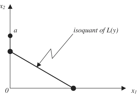
Remark on the proof of iiia): The following figure shows that when the directional
vector has all coordinates positive, for example 1 , then N xn >0,n=1, ,N is
required. In the Figure 1, input vector a has x1 = 0, and Di(y,x;1N)=0 , but a is
not on the isoquant.
x2
a isoquant of L(y)
[image:18.595.150.384.530.698.2]0 x1
This problem may be avoided by choosing the directional vector to have ones only
for positive x’s.
Proof of Theorem 1:
Assume first that the technology is as in (13), then
) , (y x
RM
{
(
)
(
x NxN)
L y n n N}
N N
n n : , , ( ),0 1, 1, ,
min ∏ 1 1/ 1 1 ∈ < ≤ =
= =
λ
λ
λ
λ
(
)
(
)
= ≤ < ≥ ∏
=min nN=1λn 1/N :Di λ1x1, ,λNxN 1,0 λn 1,n 1, ,N
(
) (
)
= ≤ < ≥ ∏
∏
=min nN=1λn 1/N : nN=1λnxn 1/N /H(y) 1,0 λn 1,n 1, ,N
(
) (
)
(
)
= ≤ < ∏
≥ ∏
∏
=min nN=1λn 1/N : nN=1λn 1/N H(y)/ nN=1 xn 1/N1,0 λn 1,n 1, ,N
(
)
1/ ( , )/ )
(y 1 x 1/ D y x
H ∏nN n N = i
= = .
Since DF(y, x) =1 /Di(y, x) we have shown that ( 3) implies RM(y, x) =DF(x, y).
To prove the converse we first show that
(
)
,0 1, 1, , ./ ) , ( )
,
(y 1x1, , x R y x 1 1/ n N
To see this,
) ,
( 1 1, , N N
M y x x
R δ δ =min
{
(
∏nN=1λn)
1/N :(λ1δ1x1, ,λNδNxN)∈L(y),}
N nn
n 1,0 1, 1, ,
0<λ ≤ <δ ≤ =
(
∏nN 1 n)
1/N min{
(
∏nN 1 n n)
1/N :( 1 1x1, , N NxN)∈L(y),= = δ − = λ δ λδ λ δ
}
N nn
n 1,0 1, 1, ,
0<λ ≤ <δ ≤ =
(
∏nN 1 n)
1/N min{
(
∏nN 1ˆn)
1/N :(ˆ1 1x1, , ˆN NxN)∈L(y),= = δ − = λ λδ λ δ
}
N n
n
n 1,0 1, 1, ,
ˆ
0<λ ≤ <δ ≤ =
(
N)
Nn n M y x
R ( , )∏ =1 −1/
= δ
where λˆn =λnδn,n=1, ,N. Thus (34) holds.
Next, assume that the Debreu-Farrell and the multiplicative Russell
measures are equal, then
(
)
( , , , )/ ) , ( )
, , ,
( 1 1 N N M nN 1 n 1/N 1 1 N N
M y x x R y x DF y x x
R δ δ = ∏ = δ = δ δ
thus
(
N)
Nn n N
N M y x DF y x x
R ( , )= ( ,δ1 1, ,δ )∏ =1δ 1/
and
(
N)
Nn n N
Nx
x y DF x y
Now we takeδn =1/xn,n=1, ,N then
(
N)
Nn n
y DF x y
DF( , )= ( ,1, ,1)∏ =1δ 1/
Moreover, since the Debreu-Farrell measure is independent of units of
measurement (Russell (1987), p. 215),11 xn can be scaled so that
N n
xn >0, =1, , . Thus by takingH(y)=DF(y,1, ,1), and using (11) we have proved our claim.
Proof of Theorem 2:
First consider
= −
− , , )
,
(y x1 1 xN N
A δ δ
, ) ( ) , , ( : 1 max
1 1 1 1
∈ − − ∑ − − =
=s x s x s L y
N N N N
N n n
δ
δ
, ) ( )) ( , ), ( ( : ) ( 1 max1 1 1 1
∈ + − ∑ − + − + =
= s x s x s L y
N N N N
N
n
n n
n δ δ δ δ
∑ + − = = N n n x y A
N 1 ( , ),
1
δ
where sn ≥0,δn ≥0,n=1, ,N.
11
This is equivalent to ∑ + = = N n n N x y A 1 1 ) ,
( δ A(y,x1−δ1, ,xN −δN)
Take δn = xn and define -F(y) =A(y,0), then since equality between the directional
distance function and the additive measure holds,
). ( 1 ) , ( ) 1 ; , ( 1 y F x N x y A x y D N n n N
i = = ∑ −
=
Next, let x∈C(L(y)), then for somex∈IsoqL(y), and
δ
≥0,. ) 1 ; ˆ , ( ) 1 ; 1 ˆ , ( ) 1 ; ,
( N = i +δ N N = i N +δ
i y x D y x D y x
D
Since xˆ∈IsoqL(y), Di(y,x;1N)=δ. Next, A(y,x) ≥ − − ∑ ∑ =
= : = ( )/ ( ) 0
1 max 1 1 y F N s x s
N n n
N n N n n ≥ − − + ∑ ∑ =
= : = (ˆ )/ ( ) 0
1 max 1 1 y F N s x s
N n n
N n N n n δ ≥ − ∑ + ∑ =
= = n N
N n N n n s N y F N x s N 1 ) ( / ˆ : 1 max 1 1 δ
= δ,