A New Eighth Order Implicit Block Algorithms for the Direct Solution of Second Order Ordinary Differential Equations

(1)

http://dx.doi.org/10.4236/ajcm.2014.44032

A New Eighth Order Implicit Block

Algorithms for the Direct Solution of

Second Order Ordinary Differential

Equations

Ademola M. Badmus

Department of Mathematics, Nigerian Defence Academy, Kaduna, Nigeria Email: [email protected]

Received 7 August 2014; revised 11 September 2014; accepted 19 September 2014

This work is licensed under the Creative Commons Attribution International License (CC BY).

http://creativecommons.org/licenses/by/4.0/

Abstract

This paper focuses on derivation of a uniform order 8 implicit block method for the direct solution of general second order differential equations through continuous coefficients of Linear Multi- step Method (LMM). The continuous formulation and its first derivatives were evaluated at some selected grid and off grid points to obtain our proposed method. The superiority of the method over the existing methods is established numerically.

Keywords

Uniform Order, Second Order Initial Value Problem, Implicit Block Algorithms, Zero Stable

1. Introduction

In the past, efforts have been made by many researchers to develop an efficient algorithm for solving second order differential equations of the form

(

, ,

) ( )

, 0 ,

( )

0

y′′= f x y y′ y =α y′ =β (1.0) directly through the interpolation and collocation points (see [1]-[4] to mention a few). Since many numerical techniques are available for the solution of higher order initial value problems (IVPs) and these techniques de-pend on many factors such as speed of convergence, computational expenses, data storage requirement and ac-curacy.

(2)

method. Seven-point solutions are obtained from the block at once which speed up the computational processes; the method is self-starting and we obtained better accuracy over the existing methods.

The Equation (1.0) where f is a continuous function, is conventionally solved by first reducing it to a system of first order differential equations and then applying the various first order methods available for their solutions. This approach is extensively discussed and established by some of the following researchers such as ([5] [6]). Also [7] [8] and [9] showed that this approach was associated with certain drawbacks. Due to the dimension of the problem after it has been reduced to a system of first order ordinary differential equations (ODEs), also the reduced systems of ODEs are not well posed unlike the given problem. The approach wastes a lot of computer time and human efforts, hence there is a great need to develop new and efficient algorithms to handle problem (1.0) directly without any reduction to its equivalent system of first order ODEs.

Several authors have also solved problem (1.0) through predictor corrector mode (PC) of implementations; among them are [10] and [11]. Although the implementation of the methods in a PC mode yields good accuracy, the approach is more costly to implement, for instance PC routines are very complicated to write, since they re-quire special techniques for supplying starting values and also predicting all the off grid points present in the method which leads to longer computer time and human efforts to handle their approach.

In our new algorithms, we take great advantage of this approach by exploring its continuous formulation na-ture to obtain some discrete schemes when evaluated at some xn j+ ,j=

[ ]

0,k to form our block method; schemes are equally obtained from the derivative of the continuous formula.

Definition 1.0

A linear multi-step method is said to be zero-stable if the roots Rj,j=1 1

( )

k of the first characteristic poly-nomials

( )

0

det 0, 1, satisfies 1

k k i

i j

i

R A R A R

ρ −

=

 

= _ _= = − ≤



∑

 .

If one of the roots is +1, we call this the principal root of ρ

( )

R (see [12]). Definition 1.1

A linear multi-step method

( )

2

( )

0 0

k k

j n j j n j

j j

y x α x y+ h β x f+

= =

=

∑

=

∑

. (1.2)

We associate the linear differential operator

( )

(

)

2

(

)

0

; ; ;

k

j j

j

L y x h α y x jh h β y x jh

=

 ′′ 

= + −

 

 

∑

  (1.3)

where y x

( )

is an arbitrary function, continuity differentiable on

[ ]

a b, .

Expanding the test function y x

(

+ jh

)

as Taylor series about x and collecting terms gives

( )

; 0

( )

1

( )

q q q

L y x h_ _=C y x +C hy x′ + + C h y x +

where C0,,Cq are constants.

A simple calculation yields the following formulae for the constants Cq in terms of the coefficients α βj, j.

(

)

(

)

(

)

₍

₎

(

)

0 0 1 2 3

1 1 2 3

2 2 2

2 1 2 3 0 1 2

2 2

1 2 3 1 2

2 3

1

2 3

2!

1 1

2 3 2 2, 3, .

! 2 !

k k

q q q q q

q k k

C

C k

C k k q

q q

α α α α α

α α α α

α α α α β β β β

α α α α β − β − β

= + + + + +

= + + + +

= + + + + − + + + +

= + + + + − + + + =

−

 



  

Hence, we say that the method has order P if C₀=C₁=C₂=C_p=C_p₊₁=0, but C_p₊₂≠0. Then C_p₊₂ is the error constant and p 2 2 2

( )

n

p p

(3)

2. Theory of Block Methods for Second Order Initial Value Problems

Within the r-vectors ym and fm (for m=nr n, =0,1,)

(

)

T 1, 2, 3, ,

m n n n n r

y = y+ y+ y+  y+

(

)

T

1, 2, 3, ,

m n n n n r

f = f + f + f +  f + .

The S block r-point methods for

( )

2

( )

0 0

k k

j n j j n j

j j

x y h x f

α ₊ β ₊

= =

=

∑

are given by the matrix finite difference equation.

( ) ( )

0 2

0 0

k k

i i

m m i m i

j j

A y A y − h B f −

= =

=

∑

+

∑

(2.0)

where A( )i,B( )i,i=0, 0

( )

are r r× matrices respectively with element aij( )i,bij( )i, for ij=0 1 .

( )

r The block scheme (2.0) is explicit if the coefficient matrix B0 is a null matrix.

Let

(

)

(

)

(

)

1

2

n

n r n n

y

y x Z

y x x₊

+

 

 

=  

 

 

 ,

be respectively the theoretical solution to Equation (1.0) (see [12] [13]).

3. Specification of the Method

We consider a power series of single variables x in the form

( )

0 j j j

P x α x

∞

=

∑

(3.0)

which is used as the basis or trial function to produce our approximate solution to (1.0) as

( )

1

0 m t

j j j

P x α x

+ −

=

∑

(3.1)

( )

1

1 1

m t j j j

P x jα x

+ − −

=

′ =

∑

(3.2)

( )

1

(

)

2

(

)

2

1 , ,

m t

j j j

P x j j α x f x y y

+ −

−

=

′′ =

∑

− = ′ (3.3)

where aj are the parameters to be determined, t and m are point of interpolation and collocation points. The

Equation (3.3) is collocated at x=xn j+ , j=

( )

0,k and interpolating (3.1) at

1 0,

2

n j

x=x₊ j= , with this method k = 3 and specifically gives the following system of non linear equations of the form h

1

0

1

, 0,

2

m t j

j n i

j

x y i

α

+ −

+ =

 

= _{=  }

 

∑

(3.4)

(

)

1

2 2

1 3 3 5

1 , 0, , ,1, , 2, , 3

2 4 2 2

m t

j

j n i

j

j j α x f i

+ −

− + =

 

− = _{= } _

 

∑

. (3.5)

(4)

( )

1 1

2 2

2

1 1 3 3 1 1 3 3 2 2 5 5 3 3

2 2 4 4 2 2 2 2

n n

n n n n n n n n

y x y y

h f f f f f f f f

α α

β β β β β β β β

+ + + + + + + + + + + + + + + + = +   = _ + + + + + + + _  

. (3.6)

When using Maple 17 mathematical software to obtain the values of αjs in (3.4), (3.5) and substituting the

values in Equation (3.0) to obtain our continuous formulation in the new method as

( )

(

)

(

)

(

)

(

)

(

)

(

)

(

)

(

)

(

)

(

)

(

)

(

)

(

)

2 3 1 2

4 5 6

2 3 4

7 8 9

5 6 6

3

2 2 1115837 1 1683

10886400 2 1620

420 5453 339

324 5400 810

413 45 2

2835 1890 1215

313243 270 1143

604800 45

n n

n n n n

n

n n n

n n n n

n n

h x x x x h

y x y y x x x x x x

h h h

x x x x x x

h h h

x x x x x x f

h h h

h

x x x x

h + − − − _ = + + −_ − + − − − + −   − − + − − − + − − − + − − + − −

(

)

(

)

(

)

(

)

(

)

(

)

(

)

(

)

(

)

(

)

(

)

(

)

4 5 2 3

6 7 8 9

1

4 5 6 6

2

3 4 5

2 3

6 7

4 5 6

957

90 75

325 740 43 4

45 315 105 135

96496 92160 32256 59392

127575 8505 1215 2025

21504 51200 3072

1215 8505 2835

n n

n n n n

n

n n n n

n n

x x x x

h h

x x x x x x x x f

h h h h

h

x x x x x x x x

h h h

x x x x

h h h

+  ₋ ₊ ₋  − − + − − − + − + − − − + −   − − + −  − +   −

(

)

(

)

(

)

(

)

(

)

(

)

(

)

(

)

(

)

(

)

(

)

(

)

(

)

8 9 3 6 4

3 4 5

2 3

6 7 8 9

1

4 5 6 6

3 4

2

2048 25515

117415 270 1413 2787

241920 36 72 120

1333 331 41 2

90 63 42 27

73279 180 501 1066

544320 81 81 135

n n

n

n n n n

n n n n n

n n n

x x x x f

h

x x x x x x x x

h h h

x x x x x x x x f

h h h h

h

x x x x x x

h h + +  − − − _ + − − + − − − + − − − + − − − + − + − − −   + − −  

(

)

(

)

(

)

(

)

(

)

(

)

(

)

(

)

(

)

(

)

(

)

(

)

(

)

5 3

6 7 8 9

3

4 5 6 6

2

3 4 5

2 3

6 7 8 9

2

4 5 6 6

2214 1184 78 8

405 567 189 243

53323 135 774 1713

1209600 180 360 600

187 265 37 2

90 315 210 135

598

n

n n n n

n

n n n n

n n n n n

x x

h

x x x x x x x x f

h h h h

h

x x x x x x x x

h h h

x x x x x x x x f

h h h h

+ + − + − − − + −      − − + −_ − +   − − − + − − − + − − − + − +

(

)

(

)

(

)

(

)

(

)

(

)

(

)

(

)

(

)

(

)

(

)

(

)

(

)

3 4 5

2 3

6 7 8 9

5

4 5 6 6

2

3 4 5

2 3

6 4

9 54 45 51

6048000 315 90 75

23 68 5 4

45 315 105 9455

34543 90 531 1223

32659200 4860 9720 16200

141 215

2430 850

n n n n

n

n n n n

n h

x x x x x x x x

h h h

x x x x x x x x f

h h h h

h

x x x x x x x x

h h h

x x h + − − − + − − − + − − − + − − −  + − − + − − − +  −  − − +   

(

)

7

(

)

8

(

)

9

3

5 6 6

33 2

5h x−xn −5670h x−xn +3645h x xn fn+   −

(3.7)

Evaluating (3.7) at 3,1, , 2, , 33 5

4 2 2

n j

x=x₊ j= and the first derivative of Equation (3.7) at x=xn, to obtain

(5)

2 2 2 2

3 1 1 3 1

4 2 2 4

2 2 2 2

3 2 5 3

2 2

1 1

2

3 1 329909 1464259 125471 774913

2 2 4644860 10321920 1088640 10321920

941669 16889 15049 43163

46448640 2580480 10321920 278691840

2 2

n n n

n n n n

n n

n

y y y h f h f h f h f

h f h f h f h f

y y y

+ + + + + + + + + + ₊ − + = + − + − + − +

− + = 2 2 2 2

1 3 1

2 4

2 2 2 2

3 2 5 3

2 2

2 2 2

3 1 1 3

2 2 2 4

057 111659 304 4177

145152 40320 1701 26880

7339 1051 13 671

181440 80640 4480 2177280

20341 23861 2792 39343

3 2

725760 40320 8505

n n

n n n n

h f h f h f h f

y y y h f h f h f

+ + + + + + + + + + + + − + − + − +

− + = + − + 2

1

2 2 2 2

3 2 5 3

2 2

2 2 2 2

2 1 1 3 1

2 2 4

2 2

3 2

2

80640

8437 16889 29 1187

181440 2580480 5760 2177280

3049 3599 4064 34163

4 3

72576 4032 8505 40320

13333 2299 181

90720 40320 2016

n

n n

n n n n

n n n

n n

h f

h f h f h f h f

y y y h f h f h f h f

h f h f

+ + + + + + ₊ ₊ ₊ + + + − + − + − + = + − +

+ + − 2 2

5 3

2

2 2 2 2

5 1 1 3 1

2 2 2 4

2 2 2 2

3 2 5 3

2 2 2 3 1 2 991 0 1088640

20149 8087 5584 9955

5 4

362880 6720 8505 8064

6367 4057 197 611

18144 13440 20160 1088640

52103

6 5

725760

n n

n n n

n n n n

n n

n

h f h f

y y y h f h f h f h f

h f h f h f h f

y y y h f

+ + + + + + + + + + + + ₊ + − + = + − + + + + +

− + = 2 2 2

1 3 1

2 4

2 2 2 2

3 2 5 3

2 2

2 2 2

1 1

2

58657 5584 23173

40320 8505 16128

23987 40657 10529 36637

36288 80640 40320 2177280

1

65318400 65318400 3347511 15851025 1439721

32659200

n n

n n n n

n

h f h f h f

h f h f h f h f

y y y h f h f h

h + + + + + + + + + + − + + + + +

′ = − − + + + ₂

2 2 2 2 2

3 1 3 3 5

2 2 4 2

34543 16915122 4396740 24702976 323406

n

n n n n

f

h f h f h f h f h f

+ + ₊ ₊ ₊ ₊  + + − − −      (3.8)

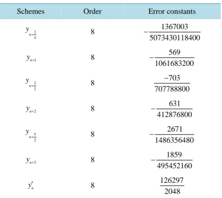
[image:5.595.207.435.517.720.2]

Equation (3.8) is our proposed uniform eighth order block method with the error constants exhibited inTable 1.

Table 1. Order and error constants of schemes (3.8).

Schemes Order Error constants

3 4 n y + 8 1367003 5073430118400 − 1 n

y₊ 8 569

1061683200 − 3 2 n y + 8 703 707788800 − 2 n

y+ 8

631 412876800 − 5 2 n y + 8 2671 1486356480 − 3 n

y+ 8

1859 495452160

−

n

y′ 8 126297

(6)

Also the first derivative of (3.7) is evaluated at 1 3, ,1, , 2, , 33 5

2 4 2 2

n j

x=x₊ j= as follows

2 2 2

1 1 1 2

2 2

2 2 2 2 2

3 1 3 3 5

2 2 4 2

3 4

1

65318400 65318400 939729 10585755 899559 32659200

21197 16257618 2802180 17537024 199854

1

8360755200 83607 4180377600

n n n n

n n

n

n n n n

n n

y y y h f h f h f

h

h f h f h f h f h f

y y h + + + + + ₊ ₊ ₊ ₊ +  ′ = − + + + +   + + − − −  

′ = − + 2 2

1 1

2

2 2 2

2 3 1

2

2 2 2

3 3 5

2 4 2

2

1 1

2

55200 117608847 1161584685

104563737 2485771 2489303394

321829620 1440166912 23361102

1

65318400 65318400 927849 32659200

n n

n

n n

n

n n n

n

y h f h f

h f h f h f

y y y h f

h + + + + ₊ + + + + ₊ + + + + +  − −    − _ 

′ = − + + 2 2

1 2

2 2 2 2 2

3 1 3 3 5

2 2 4 2

2 2 2

3 1 1 2

2 2

2

13321935 880119

20657 19061838 2768700 6754304 194994

1

65318400 65318400 880689 27057915 134919 32659200

9197

n n

n

n n n n

n n

h f h f

h f h f h f h f h f

y y y h f h f h f

h h + + + ₊ ₊ ₊ ₊ + + + +  + +    + + −    − −   ′ = − + + + + + 

2 2 2 2

3 1 3 3 5

2 2 4 2

2 2 2

2 1 1 2

2

2 2 2

3 1 3

2 2

20482578 4950780 12621824 70254

1

65318400 65318400 949449 19814895 7373079 32659200

42257 18750798 17483460 67

n

n n n n

n n n n n

n

n n

f h f h f h f h f

y y y h f h f h f

h

h f h f h f

+ ₊ ₊ ₊ ₊ + ₊ + + + ₊ ₊  + + − −   ′ = − + + + + + + +   −   2 2 3 5 4 2

2 2 2

5 1 1 2

2 2

2 2 2 2 2

3 1 3 3 5

2 2 4 2

54304 506034

1

65318400 65318400 801489 31736475 22050279 32659200

117043 22167378 8671740 17537024 5709906

n n

n n n n

n n

n

n n n n

n

h f h f

y y y h f h f h f

h

h f h f h f h f h f

y + + + + + + + ₊ ₊ ₊ ₊ +  −    ′ = − + + + +   − + + − +  

′ 2 2 2

3 1 1 2

2

2 2 2 2 2

3 1 3 3 5

2 2 4 2

1

65318400 65318400 1434729 12701745 1709559 32659200

4747697 8279118 36122820 24702976 25517646

n n n n

n

n n n n

y y h f h f h f

h

h f h f h f h f h f

+ + + + ₊ ₊ ₊ ₊    = − + + − +  + + + + +    (3.9)

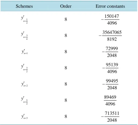
Equation (3.9) has the following order and error constants inTable 2.

4. Implementation Strategies

Equation (3.9) is substituted in Equation (3.8) when applying to Equation (1.0) directly at n=0, simultaneously produces solutions at the point 1

2 y , 3

4

y , y1, 3 2

y , y2, 5 2

(7)

[image:7.595.206.435.100.308.2]

Table 2. Order and error constants of schemes (3.9).

Schemes Order Error constants

1 2 n y

+

′ ₈ 150147

4096

−

3 4 n y

+

′ ₈ 35647065

8192

−

1 n

y′₊ 8 72999

2048

−

3 2 n y

+

′ ₈ 95139

4096

−

2 n

y′₊ 8 99495

2048

−

5 2 n y

+

′ ₈ 89469

4096

3 n

y′+ 8

713511 2048

−

for yn′ present in the method. For the advancement in the integration processes we used schemes derived at 3 4 n y

+ ,

5 2 n y

+ , yn+3 together as n=1, 2,. This new method is demonstrated on linear and non linear problems to ascertain their degree of accuracy with the existing methods.

5. Numerical Experiments

Three numerical experiments of two linear and one non linear problem were used to ascertain the efficiency of the method.

Example 1

2

6 4

0

y y y

x x

′′+ ′+ =

( )

0.1

1 1, 1 1, 0

32

y = y′ = h= x> .

Theoretical solution is

( )

5 2₄

3 3

y x

x x

= − .

Example 2

2

3 8e x

y′′− y′=

( )

0 1,

( )

0 1, 0.005

y = y′ = h= .

Theoretical solution is y x

( )

= −4e2x+3e3x+2. Example 3

2

3 8e xy y′′− y′=

( )

0 1,

( )

0 1, 0.005

y = y′ = h= .

No theoretical solution.

6. Conclusion

(8)

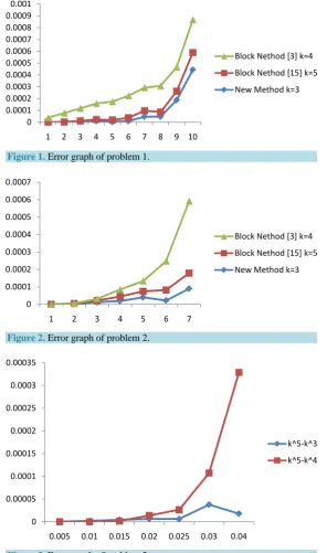
var-ious values of k are of the same order the block scheme gotten from the minimal value of k performed excel-lently well and compared favourably with the exact solutions. This has also been established for second order schemes derived from various values of k which are of the same order with three different numerical experi-ments tested (seeFigure 1,Figure 2 andFigure 3).

Table 3andTable 4 also display the numerical result of problem 1 and absolute errors by using various block

methods of k = 4, k = 5 together with the new block method at k = 3.Table 5 andTable 6 display the numerical result of problem 2 and absolute errors by using various block methods of k = 4, k = 5 together with the new block method at k = 3.

Table 7displays the approximate solution of example 3 with block methods of k = 4, k = 5 together with the

Figure 1. Error graph of problem 1.

[image:8.595.167.464.207.709.2]

0 0.0001 0.0002 0.0003 0.0004 0.0005 0.0006 0.0007 0.0008 0.0009 0.001

1 2 3 4 5 6 7 8 9 10

Block Nethod [3] k=4 Block Nethod [15] k=5 New Method k=3

0 0.0001 0.0002 0.0003 0.0004 0.0005 0.0006 0.0007

1 2 3 4 5 6 7

Block Nethod [3] k=4 Block Nethod [15] k=5 New Method k=3

0 0.00005 0.0001 0.00015 0.0002 0.00025 0.0003 0.00035

0.005 0.01 0.015 0.02 0.025 0.03 0.04

(9)

[image:9.595.86.535.101.314.2]

Table 3. Table of result for example 1.

x Theoretical solution Block method [14]k = 4 Block method [15]k = 5 New block method k = 3

1.003125 1.003076526 1.003114880 1.0030766905 1.0030764430

1.00625 1.006057503 1.006132507 1.00605684265 1.006055854

1.009375 1.008944993 1.009050907 1.0089405789 1.008938355

1.0125 1.011741018 1.011876494 1.01172802434 1.011731527

1.015625 1.014447543 1.014603110 1.014431165439 1.014480080

1.01875 1.017066494 1.017252866 1.017038197167 1.017057078

1.021875 1.019599755 1.019795810 1.01954923805 1.019553250

1.025 1.022049164 1.022270209 1.02201055468 1.0220996286

1.028125 1.024416519 1.024622147 1.02434160973 1.0242295932

[image:9.595.89.540.103.721.2]

1.03125 1.026703578 1.026981486 1.026557694498 1.027146899

Table 4. Absolute error of problem 1.

Block method [3]k = 4 Block method [15]k = 5 New method k = 3

3.8354E(−05) 1.645E(−07) 8.3E(−08)

7.5004E(−05) 6.6035E(−07) 1.16E(−06)

1.05926E(−04) 4.4141E(−06) 6.638E(−06)

1.35476E(−04) 1.299366E(−05) 9.491E(−06)

1.55567E(−04) 1.6377561E(−05) 1.9535E(−06)

1.863726E(−04) 2.8296833E(−05) 9.416E(−06)

1.96055E(−04) 5.051695E(−05) 4.6505E(−05)

2.21045E(−04) 3.860932E(−05) 4.7122E(−05)

2.0562E(−04) 7.490927E(−05) 1.86926E(−04)

2.77908E(−04) 1.458835E(−04) 4.43321E(−04)

x Theoretical solution Block method [3]k = 4 Block method [15]k = 5 New block method k = 3

0.005 1.005138526 1.005139114 1.0051388419 1.005138368

0.01 1.010558242 1.010557205 1.0105569711 1.010555066

0.015 1.016265444 1.016255068 1.0162567886 1.016252503

0.02 1.022266643 1.022226977 1.0222407282 1.022247320

0.025 1.028568067 1.028508035 1.02853411642 1.028527886

0.03 1.035176665 1.035010659 1.03511676083 1.035154590

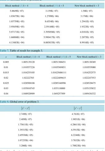
[image:9.595.91.539.567.719.2]

(10)

[image:10.595.147.487.92.579.2]

Table 6. Absolute error of problem 2.

Block method [3]k = 4 Block method [15]k = 5 New block method k = 3

5.8849E(−07) 3.159E(−07) 1.58E(−07)

1.03675E(−06) 1.2709E(−06) 3.176E(−06)

1.03759E(−05) 8.6554E(−06) 1.2941E(−05)

3.95659E(−05) 2.59148E(−05) 1.9323E(−05)

5.97171E(−05) 3.395058E(−05) 4.0181E(−05)

1.66006E(−04) 5.990417E(−05) 2.2075E(−05)

4.13483E(−04) 8.885833E(−05) 8.9916E(−05)

x Block method [3]k = 4 Block method [15]k = 5 New block method k = 3

0.005 1.005139120 1.0051388451 1.005138369

0.01 1.010557226 1.0105569851 1.010555080

0.015 1.016255105 1.01625686111 1.016252575

0.02 1.02222703 1.0222409615 1.022247553

0.025 1.028508106 1.0285346996 1.028528475

0.03 1.035010745 1.035118000 1.035155832

0.04 1.048928909 1.049257509 1.049436332

Table 8. Global error of problem 3. 5 4

y −y 5 3

y −y

2.749E(−07) 4.761E(−07)

2.409E(−07) 1.9051E(−06)

1.75611E(−05) 4.28611E(−06)

1.39315E(−05) 6.5915E(−06)

2.65936E(−05) 6.2246E(−06)

1.07255E(−04) 3.7832E(−05)

3.286E(−04) 1.78823E(−04)

Where 5 4

y −y = the absolute difference between approximate solution of k = 5 and k = 4; 5 3

y −y = the

absolute difference between approximate solution of k = 5 and k = 3.

new block method at k = 3 whileTable 8 is the global or approximate error of problem 3, since this problem has no theoretical solution.

References

[1] Yahaya, Y.A. and Badmus, A.M. (2009) A Class of Collocation Methods for General Second Order Ordinary Diffe-rential Equations. African Journal of Mathematics and Computer Science Research, 2, 69-72.

(11)

[3] Badmus, A.M. and Yahaya, Y.A. (2009) An Accurate Uniform Order 6 Block Method for Direct Solution of General Second Order Ordinary Differential Equations. The Pacific Journal of Science and Technology, 10, 248-254.

[4] Jator, S.N. (2007) A Class of Initial Value Methods for Direct Solution of Second Order Initial Value Problems. 4th International Conference of Applied Mathematics and Computing, Plovdiv, 12-18 August 2007.

[5] Lambert, J.D. (1973) Computational Methods in Ordinary Differential Equations. John Wiley and Sons, New York, 278.

[6] Lambert, J.D. (1991) Numerical Method for Ordinary Differential Systems. John Wiley and Sons, New York, 293. [7] Awoyemi, D.O. (1999) A Class of Continuous Method for General Second Order IVPs in Ordinary Differential

Equa-tions. International Journal of Computer Mathematics, 72, 29-37. http://dx.doi.org/10.1080/00207169908804832

[8] Jator, S.N. (2001) Improvements in Adams-Moulton Methods for the First Initial Value Problems. Journal of the Ten-nessee Academy of Science, 76, 57-60.

[9] Onumanyi, P., Awoyemi, D.O., Jator, S.N. and Siriseria, U.W. (1994) New Linear Multistep Methods with Continuous Coefficients for First Order IVPs. Journal of Nigeria Mathematics Society, 13, 37-51.

[10] Awoyemi, D.O. (2003) A P-Stable Linear Multistep Method for Direct Solution of General Third Order Ordinary Dif-ferential Equation. International Journal of Computer Mathematics, 80, 987-993.

http://dx.doi.org/10.1080/0020716031000079572

[11] Vigo-Angular, J. and Ramos, H. (2006) Variable Step-Size Implementation of Multi-Step Methods y′′= f x y y

(

, , ′

)

. Journal of Computation and Applied Mathematics, 92, 114-131. http://dx.doi.org/10.1016/j.cam.2005.04.043

[12] Fatunla, S.O. (1991) Block Method for Second Order Differential Equations. International Journal of Computer Ma-thematics, 41, 55-63. http://dx.doi.org/10.1080/00207169108804026

[13] Yahaya, Y.A. (2004) Some Theories and Applications of Continuous LMM for Ordinary Differential Equations. PhD Thesis (Unpublished), University of Jos, Nigeria.

[14] Badmus, A.M. and Mshelia, D.W. (2012) Uniform Order Zero Stable k-Step Block Methods for Initial Value Problems of Ordinary Differential Equations. Journal of Nigerian Association of Mathematical Physics, 20, 65-74.

[15] Badmus, A.M. (2014) An Efficient Seven Point Block Method for Direct Solution of General Second Order Ordinary Differential Equations y′′= f x y y

(

, , ′

)

. British Journal of Mathematics and Computer Science, 4, 2840-2852.

(12)