Preferential attachment and growth dynamics in complex systems

Munich Personal RePEc Archive

Preferential attachment and growth

dynamics in complex systems

Yamasaki, Kazuko and Matia, Kaushik and Buldyrev, Sergey

V. and Fu, Dongfeng and Pammolli, Fabio and Riccaboni,

Massimo and Stanley, H. Eugene

IMT Institute For Advanced Studies, Lucca

26 June 2004

Online at

https://mpra.ub.uni-muenchen.de/15908/

Preferential attachment and growth dynamics in complex systems

Kazuko Yamasaki1,2_{, Kaushik Matia}2_{, Sergey V. Buldyrev}2_{, Dongfeng}

Fu2_{, Fabio Pammolli}3_{, Massimo Riccaboni}3 _{and H. Eugene Stanley}2

1_{Tokyo University of Information Sciences, Chiba City 265-8501 Japan.}

2_{Center for Polymer Studies and Department of Physics,}

Boston University, Boston, MA 02215 USA.

3_{Faculty of Economics, University of Florence and CERM,}

Via Banchi di Sotto 55, Siena 53100 Italy.

Abstract

Complex systems can be characterized by classes of equivalency of their elements defined

accord-ing to system specific rules. We propose a generalized preferential attachment model to describe

the class size distribution. The model postulates preferential growth of the existing classes and the

steady influx of new classes. According to the model, the distribution changes from a pure

expo-nential form for zero influx of new classes to a power law with an expoexpo-nential cut-off form when

the influx of new classes is substantial. Predictions of the model are tested through the analysis of

a unique industrial database, which covers both elementary units (products) and classes (markets,

firms) in a given industry (pharmaceuticals), covering the entire size distribution. The model’s

predictions are in good agreement with the data. The paper sheds light on the emergence of the

Many diverse systems of physics, economics, and biology [1–5], share in their growth

dy-namics two basic similarities: (i) The system does not have a steady state and is growing. (ii)

Basic units are born and they agglomerate to form classes. Classes grow in size preferentially

depending on the existing size. In the context of economic systems, units are products, and

the classes are firms. In social systems units are human beings, and the classes are cities.

In biological systems units can be bacteria, and the classes are the bacterial colonies.

The probability distribution function p(k) of the class size k of the systems mentioned

above share a universal behavior p(k)∼k−τ

with τ ≈2 [1, 3, 4, 6]. Other possible values of

τ are discussed and reported in [7]. Also, for most of the systems p(k) has an exponential

cutoff which is often assumed to be a finite size effect of the databases analyzed. Several

models [2, 9–13] explain τ ≈ 2 but none explains the exponential cutoff of p(k). Moreover,

these models describing p(k) ∼ k−τ

are not suitable to describe simultaneously systems

for which p(k) ∼ exp(−γk). Here we present a model with simple set of rules to describe

p(k) for the entire range of k, i.e., power law with an exponential cutoff. We show that

the exponential cutoff of the power law is not due to finite size but an effect of the initial

conditions from which the system starts to evolve. We also show that the functional form

of p(k) depends on the initial conditions of our model and changes from a pure exponential

to a pure power law (with τ = 2) via a power law with an exponential cutoff. We justify

our model by empirical analysis of a recently constructed pharmaceutical industry database

(PHID) [14, 15].

We now present a model, which has the following rules:

1. At time t = 0 there existsN classes, each with a single unit.

2. At each simulation step:

• (a) With probabilityb (0≤b≤1) a class with a single unit is born.

• (b) With probability λ (0< λ≤ 1) a randomly selected class grows one unit in

size. The selection of the class that grows is done with probability proportional

to the number of units it already has [“preferential attachment”].

• (c) With probability µ (0 < µ ≤ 1, µ < λ) a randomly selected class shrinks

one unit in size. The selection of the class that shrinks is done with probability

In the continuum limit the proposed growth mechanism gives rise to a master equation of

p(k, ti, t) which is the probability, for a classi born at simulation step ti, to have k units at

step t:.

∂p(k, ti, t)

∂t =λ

(k−1)

g(t) p(k−1, ti, t)

+µ(k+ 1)

g(t) p(k+ 1, ti, t)−(λ+µ)

k

g(t)p(k, ti, t)

(1)

whereg(t)≡N+(λ−µ+b)tis the total number of units at simulation steptandp(1, ti, ti) =

1. Equation (1) is the generalization of the master equation of birth and death processes [12].

The analytical solution of Eq. (1) is given by

p(k, t) = N

N +btp(k,0, t), + b N +bt

Z t

0

dtip(k, ti, t) (2)

where the functional form of p(k, ti, t) is given in [8]. The lengthy derivation of the full

solution of eq. 1 which is a power law(the second term of eq. 2) with an exponential cutoff

(the first term of eq. 2) will be presented elsewhere, here we present simulation results.

First we discuss two limiting solutions of Eq. (1).

• Case i : No new classes are born (b = 0). The growth of the system is solely due to

the preferential attachment of new units to the pre-existing N classes. In this case

(Fig 1a) [12]

p(k)∼e− kN

t(λ−µ). (3)

This limiting case can be considered as one of the initial condition of the model where

birth or death of classes arenotallowed. We observe that this initial condition results

in a pure exponential distribution of the number of units inside classes.

• Case ii : At t = 0, N = 0, and new classes are born with probability b 6= 0. In this

case, for large times p(k) is a pure power law

p(k)∼k−τ

, τ = 2. (4)

This limiting case can be considered as another different initial condition of the model

where birth or death of classes are allowed starting from N = 0 classes. We observe

that this initial condition results in a pure power law distribution of the number of

This case is identical to the Simon model [13] and can be understood by the following

arguments. From case (i) we know that when the number of classes remains constant,

p(k) decays exponentially with k. The power law of case (ii) is the effect of

superposi-tion of many exponentials with different decay constants, each resulting from classes

born at different times (Fig 1a).

We next present a mean field interpretation of the result τ ≈ 2. At any moment t0 the

number of units in the already-existing classes is g(t0). Suppose a new class consisting of

one unit is created at time t0. According to rules 2b, 2c, the growth rate is proportional

to 1/g(t0). Neglecting the effect of the influx of new classes on g(t0), the average size k

of this class born at t0 is proportional to 1/g(t0). So the classes which were born at times

t > t0 remain smaller than the classes born earlier. If we sort the classes according to their

size, the rank R(k) of a class is proportional to the time of its creation R(k) ∝ t0. Thus

k ∼1/g(t0)∼1/t0 ∼1/R(t0) and we arrive to the standard formulation of the Zipf’s law [4]

according to which the size of a class k is inversely proportional to its rank. If we take into

account the decrease of the growth rate with the influx of new classes, one can show after

some algebrak∼R−(λ−µ)/(λ−µ+b)

, which includesk ∼R−1

as a limiting case forb→0. Since

R(k) is the number of classes whose size is larger than k, we can write in the continuum

limit R(k)∼R_k∞p(k)dk and hence p(k)∼k−2−b/(λ−µ)

.

The full solution of Eq. (1), a power law with an exponential cutoff, can be interpreted

using the following arguments. We start with N classes which are colored red, and let the

newly born classes be colored blue. Due to the preferential attachment rule, the red classes

remain on average larger than the blue classes. Thus for large k, p(k) is governed by the

exponential distribution of the red classes (Case i) while for smallk,p(k) is governed by the

power law distribution of the blue classes (Case ii) (Fig. 1b).

Now we apply this model to describe the statistical properties of growth dynamics of

business firms in pharmaceutical industry. PHID records quarterly sales figures of 48 819

pharmaceutical products commercialized in the European Union and North America from

September 1991 to June 2001. The products in PHID can be classified in five different

hierarchal levels A, B, C, D, and E (Fig. 2) [16]. Each level has a different number of

classes, and different initial conditions (Table I).

We observe that there are positive correlations between the number of units (products)

hierarchal level (Table II). This empirical observation supports preferential birth or death

mechanism (rules 2b, 2c) used in our model.

For levels A and B where the number of classes did not change we obtain an exponential

distribution (Figs. 3a, 3b) as predicted by limiting Case i of the model. For levels C and

D a weak departure from the exponential functional form [Figs. 3c, 3d] is due to the slight

growth in the number of classes.

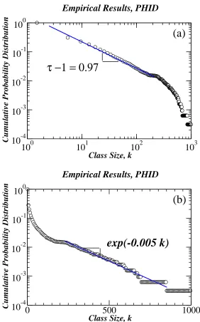
The full solution predicted by our model, i.e., the initial power law followed by the

exponential decay ofp(k) is observed empirically for level E (Fig. 4). For level E we observe

a power law with τ = 1.97 for k < 200, and an exponential cutoff for k > 200. From

the discussion above with red and blue classes we may infer that the exponential part of

p(k) arises from pre-existing firms, while the power law part of p(k) represents the young

firms that enter the market. We conclude by noting that our model is in agreement with

empirical observation where we observe p(k) to be pure exponential or a power law with an

exponential cutoff. Our analysis also sheds light on the emergence of the exponent τ ≈ 2

Level A B C D E

total number of 13 84 259 432 3913

classes in each levels

number of classes 0 0 8 20 458

born in each level

number of classes 0 0 0 0 252

died in each level

TABLE I: Two different initial conditions for classes in PHID levels: (i) For levels A and B we

have no birth or death of classes. System grows with the birth or death of units to pre-existingN

classes (13 for level A and 84 for level B). (ii) For levels C and D system grows not only with the

birth or death of classes but also with birth and death of units inside classes.

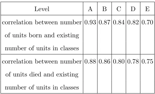
Level A B C D E

correlation between number 0.93 0.87 0.84 0.82 0.70

of units born and existing

number of units in classes

correlation between number 0.88 0.86 0.80 0.78 0.75

of units died and existing

number of units in classes

TABLE II: Correlation of birth and death of units with existing number of units in classes for each

level in PHID. This observed correlation justifies the preferential birth or death of units which is

rule 2 b and 2 c of our model.

[1] H. Jeong, B. Tomber, R. Albert, Z. N. Oltvai, and A. L. Barab´asi,Nature 407_{, 651 (2000).}

[2] S. V. Buldyrev, N. V. Dokholyan, S. Erramilli, M. Hong, and J. Y. Kimet al.,Physica A330_,

653 (2003).

[3] M. Batty and P. Longley, Fractal Cities(Academic Press, San Diego, 1994).

[4] G. Zipf, Human behavior and the principle of last effort (Addison-Wesley, Cambridge, 1949).

(1998).

[6] R. Kumar, P. Raghavan, S. Rajagopalan, and A. Tomkins,Comput. Netw. 31_{, 1481 (1999).}

[7] M. E. J. Newman, preprint condmat/0412004.

[8] p(k, ti, t) = (1−ηti,t)(1−

µ ληti,t)η

k−1

ti,t , and ηti,t = 1−

„

ti+N(λ−µ+b)−1

t+N(λ−µ+b)−1

« (λ−µ)

(λ−µ+b)

1−µ

λ „

ti+N(λ−µ+b)−1

t+N(λ−µ+b)−1

« (λ−µ)

(λ−µ+b)

[9] D. Champernowne, Economic Journal63_{, 318 (1953).}

[10] J. Fedorowicz, Journal of American Society of Information Science 33_{, 223 (1982).}

[11] X. Gabaix (1999), Quarterly Journal of Economics114_{, 739 (1999).}

[12] W. J. Reed and B. D. Hughes,Phys. Rev. E 66_{, 067103 (2002).}

[13] Y. Ijiri and H. A. Simon, Skew distributions and the sizes of business firms (North-Holland

Pub. Co., Netherlands, 1977).

[14] G. De Fabritiis, F. Pammolli, M. Riccaboni, Physica A324_{, 38 (2003).}

[15] K. Matia, D. Fu, S. V. Buldyrev, F .Pammolli, M. Riccaboni and H. E. Stanley EPL67 ₄₉₈

(2004).

[16] The different levels A, B, C, D of PHID are the four different anatomical therapeutic chemical

(ATC) levels. Classes in ATC 1 are organs of the body, classes in ATC 2 are therapeutic

preparations, classes in ATC 3 and 4 are the chemicals and compounds respectively used in

10

10

10

10

10

Class Size, k

10

10

10

10

10

10

Cumulative Probability Distribution

b=0; no new class creation N=0; system starts with 0 class

Simulation

τ −1 = 1

exp (-0.01)

(a)

100 101 102 103

Class size, k

10-4 10-3 10-2 10-1 100

Cumulative Probability Distribution

0.05%

10%

20%

50%

80%

100%

Simulation

percentage of pre-existing classes to new classes

(b)

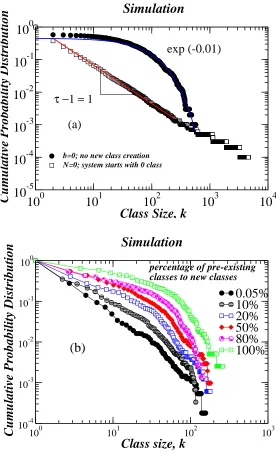
FIG. 1: Simulation results of the model. (a) Symbols are data points from simulation, solid lines

are regression fits. We observe forb= 0 (i.e. no class creation ) cumulative probability distribution

is a pure exponential while forN = 0 (i.e. we start with zero initial class ) a pure power lawk−(τ−1)

with exponentτ = 2. (b) We observe that as we change the ratio of number of pre-existing classes

Level C: 259 classes

Level A : 13 classes

Level D: 432 classes

Total 48819 products

Level E: 3913 classes

PHID ( hierarchal classification )

Level B: 84 classes

FIG. 2: In the pharmaceutical industry, products can be classified according to five levels. When

a particular product arrives in the market, it is labeled under any one of the 13 classes of the level

A, 84 classes of level B, and so on. Since the 19th century, the number of classes of level A or B has

remained constant even though the number of products within each class had a dramatic growth.

Over the period of our empirical analysis the number of classes in levels C and D increased by 3%

and 5% respectively. Products can also be grouped into firms which markets them (classification

0 2000 4000 6000 8000 10000

10

10

exp( -0.00031 k )

0 500 1000 1500 2000 2500 3000

10

10

10

exp( -0.0015 k )

0 500 1000 1500

10

10

10

10

_{exp( -0.0039 k )}

0 500 1000 1500

10

10

10

10

_{exp( -0.0044 k )}

(a)

(b)

(c)

_(d)

ClassSize, k

Cumulative Probability Distribution

Empirical Results, PHID

FIG. 3: Figures (a)∼(d) corresponds to levels (A)∼(D) respectively. Products in the pharmaceuti-cal industry are classified into levels A, B, C and D. Levels A and B have fixed numbers of classes,

the number of classes in levels C and D increases by 3% and 5% respectively over the period of

our analysis. For instance, for level A (fig. 3 a) which contains only 13 classes, the distribution is

estimated from 13 random interger numbers which corresponds to classifying 48,819 products in

13 classes. Symbols represent data points in each level (a)∼(d) while solid lines are predictions of the model. Cumulative probability distributions for all levels are pure exponentials as predicted

10

10

10

10

Class Size, k

10

10

10

10

10

Cumulative Probability Distribution

Empirical Results, PHID

τ −1 = 0.97

(a)

0

500

1000

Class Size, k

10

10

10

10

10

Cumulative Probability Distribution

Empirical Results, PHID

exp(-0.005 k)

(b)

FIG. 4: Empirical results from PHID level E. The classes analyzed here are the firms. Circles are

data points, solid lines are regression fits. (a) Log-log plot of cumulative probability distribution

of the class sizes show a power law decay k−(τ−1)